Semiclassical quantization
using Bogomolny’s quantum surface of section

Abstract

The efficacy and accuracy of Bogomolny’s method of the quantum surface of section is evaluated by applying it to the quantization of the motion of a particle in a smooth 2-D potential. This method defines a transfer operator $T$ in terms of classical trajectories of one Poincaré crossing; knowledge of $T$ provides information about the eigenstates of the quantum system. By using a more robust quantization criterion than the one proposed by Bogomolny, we are able to locate more than five hundred quantum states in both the regular and the chaotic regimes—in most cases unambiguously—and see no reason that the spectra could not be continued indefinitely. The errors of the predictions are comparable in the two regimes, and roughly constant for increasing excitation, but grow as a fraction of the (shrinking) mean level spacing. We also show computed surface of section wavefunctions, and present other theoretical and practical results related to the technique.

Contents

toc

I Introduction

Semiclassical methods of quantizing certain types of Hamiltonian systems have been known since the discovery of quantum mechanics. Specifically, if a Hamiltonian is classically integrable (if it has as many constants of motion as degrees of freedom) then its trajectories are constrained to invariant tori, and EBK quantization can be applied. Quantization occurs when the action integrated along any closed loop on one of these tori satisfies

$\displaystyle\oint_{C_{i}}p\cdot dq=2\pi\hbar(n_{i}+\mu_{i}/4)\;,$

where $\mu_{i}$ is an integer that counts the number of caustics along the trajectory. For 1-D Hamiltonians (all of which are integrable), the tori are just the periodic orbits, and the analogous WKB method can be applied; it yields accurate results with little effort, even for the ground state. However, integrable systems form only a subset of measure zero of all Hamiltonians systems; the fact that most famous and textbook examples are of the integrable sort is because they are easier to handle, not because nonintegrable systems are intrinsically less interesting.

Steps towards understanding how to quantize generic, nonintegrable systems semiclassically are more recent. The approach that currently dominates the field is the trace formula of Gutzwiller, which sums purely classical information about periodic orbits into an expression for the quantum mechanical density of states; the poles of the expression indicate quantum eigenenergies [2, 3, 4, 5]. However, the number of periodic orbits increases exponentially with period—faster than the contributions of individual orbits decrease; thus the sum does not converge absolutely. A large volume of current research is devoted to developing clever tricks to reorder the sum in such a way that it converges to a useful answer, but the problem is not yet satisfactorily solved.

Recently, Bogomolny proposed an entirely different scheme to obtain eigenstate information in the semiclassical limit by using a quantum surface of section (SOS) [6]. His method, which is the topic of this paper, will be specified precisely and discussed at length in subsequent sections; for now, we will try to present a conceptual overview while avoiding unnecessary details.

A quantum surface of section is akin to the classical Poincaré surface of section, which has proven so useful to classical dynamicists both practically and theoretically. A classical Poincaré SOS is a surface drawn through a system’s phase space; the trajectory of interest is computed and each time that it pierces the surface in a prespecified direction, the point where the crossing occurred is noted. The pattern of points produced by a succession of crossings gives information about the nature of the trajectory—for example, whether it is periodic, quasi-periodic, or chaotic. SOS’s are most useful for systems that have two degrees of freedom; such a system has a four dimensional phase space and a three dimensional energy shell, but only a two dimensional surface of section (the most convenient dimension for plotting and viewing).

Bogomolny’s quantum surface of section is similarly a surface drawn through the configuration space of the corresponding classical Hamiltonian. Again classical trajectories are integrated from one crossing until the next same-direction crossing of the surface. But now, instead of only marking the points where the trajectories cross the surface, one also notes the semiclassical phase $\exp(iS/\hbar)$ which has accumulated since the previous crossing ($S=\int\vec{p}\cdot d\vec{q}$ is the action accumulated along the trajectory). Such information, for all classical orbits of one Poincaré mapping and some energy $E$, is summed together and projected onto the coordinate part of the SOS into a transfer operator $T$ which will be defined below. The projection process discards the momentum information normally associated with a classical surface of section, and $T$ correspondingly operates on functions of one variable fewer than the number of degrees of freedom in the system (namely, the Poincaré section’s position coordinates).

Since $T$ requires only information about trajectories of one Poincaré mapping, it is well defined in terms of only finite quantities. Therefore, there are no problems at all, neither theoretical nor practical, with divergences in Bogomolny’s technique. The $T$ matrix can be computed to arbitrary accuracy, requiring (as we shall see) only a two dimensional numerical quadrature of finite-time orbits. This very attractive attribute is one that is not posessed by the Gutzwiller trace formula, which is plagued by the exponentially growing number of periodic orbits of increasing period.

Conceptually, $T$ gives the evolution of a quantum mechanical wave function from one intersection with the SOS to the next. In this regard $T$ is akin to a Green function in the energy representation. $T$ operates on functions $|\psi\rangle$ which live on the coordinate part of the surface of section:

$\displaystyle|\psi^{\prime}\rangle=T|\psi\rangle\;.$

$|\psi\rangle$ has the value of the full quantum mechanical wavefunction where the latter intersects the surface of section. $T$ applied to $|\psi\rangle$ produces, roughly speaking, the image of $|\psi\rangle$ after one Poincaré mapping. Eigenstates of the quantum system occur for values of adjustable parameters (which we call $\alpha$, but could be for example $E$ or $\hbar$) for which $T_{\alpha}$ has an invariant state

$$T_{\alpha}|\psi\rangle=|\psi\rangle;$$ (1)

i.e., they occur whenever $T_{\alpha}$ has an eigenvalue that is equal to unity. So to find the eigenstates of a quantum mechanical system, one computes $T$, diagonalizes it to find its eigenvalues, and plots those eigenvalues in the complex plane for a range of $\alpha$. Whenever one of the eigenvalues crosses through $1$, then at the corresponding set of parameters $\alpha$, the quantum mechanical system is predicted to have an eigenstate.

We know of four other calculations to date that use Bogomolny’s technique. Lauritzen [7], by resorting to a stationary phase integral, showed that Bogomolny’s quantization condition (1) reduces to EBK quantization for integrable systems in general, and the rectangular billiard in particular. Bogomolny and Carioli [8] applied the method to a “surface of constant negative curvature” with vanishing potential energy; this is a billiard-type chaotic system whose orbits can also be written explicitly.

Szeredi, Lefebvre, and Goodings [9] used the quantum SOS in their study of the wedge billiard, a scalable system bounded on two sides by straight hard walls and confined in the open direction by a uniform downward gravity-like force. This system has four types of orbits of one Poincaré mapping, which can be written down; they summed these orbits into a $T$ matrix in a basis of position-space cells and were able to reproduce the first twenty quantum eigenvalues with an average RMS error of 6.5% of the mean level spacing.

Finally, Boasman in his thesis [10] thoroughly investigates, in a largely analytic way, the asymptotic accuracy that Bogomolny’s method achieves for billiard problems, and supports his predictions with evidence from numerical calculations.

Each of the previous calculations were restricted to non-generic systems—integrable systems or billiards (or integrable billiards). There is, of course, a reason for preferring billiards: they are scalable systems whose classical trajectories are the same regardless of energy, many chaotic billiards are known, and, most importantly, one can write down explicit formulas for the classical trajectories connecting any two points on the surface of section. On the other hand, billiards are thought to have different convergence properties than smooth potentials [11]. Moreover, smooth potentials—not billiards—are the kind typically encountered in models of natural systems, so it is interesting to know how well they can be handled with new methods.

Therefore, we chose to undertake our research in this more challenging laboratory—the smooth Hamiltonian system. The centerpiece of this paper is a computational application of Bogomolny’s method to the Nelson₂ potential (see Appendix A), a smooth, bounded, nonlinear oscillator with Hamiltonian

$\displaystyle H={1\over 2}\left(p_{x}^{2}+p_{y}^{2}\right)+{1\over 2}\omega^{2}x^{2}+{1\over 2}\left(y-{1\over 2}x^{2}\right)^{2}\;.$

The system is non-scalable and has a rich periodic orbit structure [12]. For low energies, it approaches a 2-D anisotropic harmonic oscillator and is predominantly regular; as the energy is increased, the degree of chaos increases and eventually dominates the phase space. We will present computations in both regimes to illuminate the similarities and differences.

This paper is organized as follows: Section II A outlines the idea of Bogomolny that is the subject of this paper. Section II B develops various expressions for $T$ which offer a somewhat different perspective on its operation, and which translate directly into a quadrature algorithm for computing $T$ in a non-billiard system. Section II C shows how to take advantage of a mirror symmetry when computing $T$. Section II D estimates the effort needed to apply Bogomolny’s method, as compared with traditional methods. Section II E explains a trick which enables Bogomolny’s theory to be verified with less numerical effort than a naive approach would require. Section III discusses the nature of eigenclassicity problems in general, and provides details of how the exact eigenclassicity spectrum was calculated for the Nelson₂ system. Section IV A introduces the model system to which we applied Bogomolny’s method. Section IV B gives some of the behind-the-scenes details about our implementation of the semiclassical computation. Section IV C qualitatively describes the behavior of the eigenvalues of the $T$ operator. Section IV D presents the eigenclassicity spectra produced by Bogomolny’s method, and compares them to exact spectra in both the regular and the chaotic regime. Finally, section IV E tells how the surface of section wavefunctions can be obtained from the theory, and makes some comments about how well they are predicted.

A comment about nomenclature: we will be dealing with two related but distinct eigenproblems—Bogomolny’s condition on the $T_{\alpha}$ operator (Eq. (1)) and the time independent Schrödinger equation for the full quantum mechanical system. In order to reduce confusion, we assume the following naming convention: the terms eigenvalues and surface of section eigenfunctions in this paper always refer to quantities obtained from diagonalizing the $T_{\alpha}$ operator. It should be kept in mind that $T_{\alpha}$ and its eigenvalues can be computed for any choice of parameters $\alpha$, whether or not an eigenstate of the quantum system exists for those parameters. The words eigenenergies, eigenclassicities (explained below), and eigenstates all refer to energy eigenstates of the full quantum mechanical Hamiltonian. These eigenstates only exist for special values of the parameters $\alpha$—in fact, only those for which $T$ has a unit eigenvalue, according to Bogomolny’s theory.

II Theory

A The results of Bogomolny

Bogomolny [6] gives an expression for the transfer operator $T$ for systems of any dimension and using any surface of section. Our interests are narrower, since the systems for which we will be doing computations are symmetric about the $y$-axis, and the $y$-axis will be used as the surface of section. In this case, the expression for $T$ can be written

$$\langle y^{\prime}|T|y\rangle=\frac{1}{(2\pi i\hbar)^{1/2}}\sum_{\rm cl.tr.}\left|\partial^{2}S(y^{\prime},y)\over\partial y\partial y^{\prime}\right|^{1/2}e^{-i\pi\nu/2}\exp i\frac{S(y^{\prime},y)}{\hbar}\;.$$ (2)

$T$ can be calculated for any chosen value $E$ of energy. The sum is over all classical trajectories which have that energy and start at $(0,y)$ and end at $(0,y^{\prime})$ one Poincaré mapping later (that is, with no intervening same-direction piercings of the SOS) (See Fig. 1).

FIG. 1.: Orbits which contribute to the semiclassical transfer operator. In Bogomolny’s construction, the trajectories which contribute are those of one complete Poincaré section: they are integrated from one intersection with the $y$-axis until the next intersection that occurs in the same direction.

$S(y^{\prime},y)\equiv\int_{y}^{y^{\prime}}\vec{p}\cdot d\vec{q}$ is the classical action along the trajectory considered. The second derivative of $S$ gives the degree of focusing of nearby trajectories onto the current trajectory. The focusing switches sign each time that there is a perfect re-convergence of nearby trajectories, which would lead to a branch cut ambiguity when its square root is taken; therefore, its absolute value is taken and the phase is put in separately through the Maslov index $\nu$, which counts the number of sign changes in the focusing (note: its role is a bit subtler in higher dimensions; see Ref. [13]).

Bogomolny’s construction of the $T$ operator begins by dividing the allowed portion of phase space into two subregions “1” and “2,” one on either side of the surface of section. In each half, a Green function $G_{1,2}$ is constructed which (i) obeys Schrödinger’s equation in that subregion, (ii) is arbitrary on the SOS, and (iii) obeys the same boundary conditions as the true wavefunctions on the remainder of the boundary of that subregion. The next step is to write the wavefunctions in terms of the Green functions and a source function $\psi_{1,2}(y)$ on the surface of section:

$\displaystyle\Psi_{1,2}(x,y)=\int_{\Sigma}dy^{\prime}\,G_{1,2}(x,y;y^{\prime};E)\psi_{1,2}(y^{\prime})\;.$

This equation, plus the demand that $\Psi_{1}$ and $\Psi_{2}$ match on the SOS and satisfy the Schrödinger equation in region 1 or 2, respectively, lead to the self-consistency requirement that $\psi_{1}(y)$ satisfy

$$\int_{\Sigma}dy^{\prime}\,\tilde{G}(x,y;y^{\prime};E)\psi_{1}(y^{\prime})=0$$ (3)

where

$$\tilde{G}(x,y;y^{\prime};E) = \frac{\hbar^{2}}{2}\int_{\Sigma}dy^{\prime}$$

$$\times\left(G_{1}(0,y;y^{\prime};E)\frac{\partial}{\partial n}G_{2}(x,y;y^{\prime};E)-G_{2}(x,y;y^{\prime};E)\frac{\partial}{\partial n}G_{1}(0,y;y^{\prime};E)\right)$$

and $n$ is the outward-directed normal at point $(0,y)$.

For points on the surface of section, it is straightforward to write the expression for $\tilde{G}$ in the semiclassical limit in terms of a sum over classical trajectories of one Poincaré mapping:

$$\tilde{G}(y^{\prime\prime};y^{\prime};E) = \sum_{\rm cl.tr.}\frac{1}{i\hbar(2\pi i\hbar)^{1/2}}\left|\frac{1}{|p^{\prime\prime}|\,|p^{\prime}|}\frac{\partial^{2}S}{\partial y^{\prime\prime}\partial y^{\prime}}\right|^{1/2}$$

$$\times\exp\left(\frac{i}{\hbar}S(y^{\prime\prime},y^{\prime};E)-i\frac{\pi}{2}\nu\right)\;.$$

A few more unilluminating steps transform the consistency condition (3) into

$\displaystyle\det(1-T)=0\;,$

where $T$ is given by Eq. (2).

Bogomolny also gives some of the properties of the $T$ operator, and proves them in the classical limit $\hbar\rightarrow 0$. His most important of these subsidiary claims is that in the limit $\hbar\rightarrow 0$, the $T$ operator is unitary. This is, to be sure, a strange sort of unitarity, in light of his other claim that the dimension of $T$ varies smoothly with parameters (such as energy); specifically, he says that

$$\dim T_{\alpha}=\frac{\text{volume of allowed region on Poincar\'{e} surface}}{(2\pi\hbar)}\;.$$ (4)

The mechanism by which these two phenomena coexist will be examined in detail in the context of our numerical experiment (Sec. IV C).

There are other interesting subjects covered in Bogomolny’s paper, such as the relationship between $T$ and the Selberg zeta function, and his prescription for computing full quantum mechanical eigenfunctions; we will not address those challenges in this paper, beyond presenting computations of surface of section wavefunctions predicted by the theory and comparing them to the exact SOS wavefunctions.

B Computing the $T$ operator: Avoiding the shooting problem

Each of the coordinate-space matrix elements of $T$ in expression (2) above is a sum over classical trajectories of energy $E$ which go from $(0,y)$ to $(0,y^{\prime})$ in one Poincaré mapping. But to find these trajectories, it would be necessary to find all values of the initial momentum $\vec{p}=(p\cos\theta,p\sin\theta)$ that cause a trajectory launched from $y$ to next intersect the SOS at $y^{\prime}$. Even though the momentum magnitude $p=\sqrt{2(E-V(0,y))}$ is fixed by the choice of energy, one would still have to solve a shooting problem—a (numerical) search in $\theta$ space to find the launching angles which cause the particle to end up at $y^{\prime}$.

But this can be avoided. Consider: any properly chosen surface of section has the property that every trajectory eventually pierces it. As a function of initial conditions (on the SOS), call the next crossing point $Y^{\prime}(y,\theta,E)$. It follows that every trajectory of the appropriate energy contributes to $T$; if it starts at $(0,y)$ with angle $\theta$, for example, it contributes to $\langle Y^{\prime}(y,\theta,E)|T|y\rangle$. This observation suggests that we transform (2) from a sum over endpoints into an integral over initial conditions.

Executing the desired transformation is possible and indeed straightforward. First we write a more useful expression for the partial derivative which appears in Eq. (2), being explicit about which variables are held constant:

$$\frac{\partial^{2}S(y^{\prime},y)}{\partial y\partial y^{\prime}} \equiv \left[{\partial\over\partial y^{\prime}}\left(\partial S(y^{\prime},y)\over\partial y\right)_{y^{\prime}E\Sigma}\right]_{yE\Sigma}$$

$$= \left[{\partial\over\partial y^{\prime}}(-p_{y})\right]_{yE\Sigma}$$

$$= -\left[\partial y^{\prime}\over\partial p_{y}\right]_{yE\Sigma}^{-1}\;.$$

Here we use a subscript of “$\Sigma$” to remind ourselves that the surface of section is meant to be fixed during the differentiation—in our case, $x=x^{\prime}=0$. The second line follows from the well-known identity $\left(\partial S/\partial y\right)_{y^{\prime}E}=-p_{y}$.

As a function of initial conditions $y$ and $\theta$,

$$\left[\partial y^{\prime}\over\partial p_{y}\right]_{yE\Sigma} = \left[\partial Y^{\prime}(y,\theta,E)\over\partial p_{y}\right]_{yE\Sigma}$$

$$= \left[\partial Y^{\prime}\over\partial\theta\right]_{yE\Sigma}\left[\partial\theta\over\partial p_{y}\right]_{yE\Sigma}$$

$$= {1\over p_{x}}\left[\partial Y^{\prime}\over\partial\theta\right]_{yE\Sigma}\;.$$

Substituting into Eq. (2) and integrating out the basis states on the LHS, we have

$$T={1\over(2\pi i\hbar)^{1/2}}\int dy\int dy^{\prime}\sum_{\rm cl.tr.}|p_{x}|^{1/2}\left|\partial Y^{\prime}\over\partial\theta\right|_{yE\Sigma}^{-1/2}e^{iS/\hbar-i\pi\nu/2}|y^{\prime}\rangle\langle y|\;.$$ (5)

Now we notice that the sum over classical trajectories that go from $y$ to $y^{\prime}$ in one Poincaré mapping is equivalent to a sum over the discrete values $\theta_{i}$ that solve the shooting problem $y^{\prime}=Y^{\prime}(y,\theta_{i},E)$ for the present values of $y$, $y^{\prime}$, and $E$. Schematically, we express that statement with the following equalities, which hold no matter what expression is inserted in the braces:

$$\sum_{\rm cl.tr.}\biggl{\{}\ldots\biggl{\}} = \int d\theta\sum_{i}\delta(\theta-\theta_{i})\left.\biggl{\{}\ldots\biggl{\}}\right|_{\theta}$$

$$= \int d\theta\left|\partial Y^{\prime}(y,\theta,E)\over\partial\theta\right|_{yE\Sigma}\delta(y^{\prime}-Y^{\prime}(y,\theta,E))\left.\biggl{\{}\ldots\biggl{\}}\right|_{\theta}\;.$$

When we apply this identity to Eq. (5), the $\delta$-function allows us to do the $y^{\prime}$ integral immediately:

$$T = {1\over(2\pi i\hbar)^{1/2}}\int dy\int d\theta\,|p_{x}|^{1/2}\left|\partial Y^{\prime}(y,\theta,E)\over\partial\theta\right|_{yE\Sigma}^{1/2}$$ (7)

$$\times\exp\left(i\frac{S(y,\theta)}{\hbar}-i\frac{\pi}{2}\nu\right)|Y^{\prime}(y,\theta,E)\rangle\langle y|\;.$$

The result is an expression for $T$ which can be evaluated without solving any shooting problems—a reduction of numerical effort. Moreover, this expression more closely represents our intuitive picture of the effect of $T$ than Eq. (2); that is, when $T$ is applied to an initial surface of section wavefunction $|\psi\rangle$,

1. it breaks up $|\psi\rangle$ into its components at each position $y$;

2. each of these components becomes an ensemble of classical particles, launched in all directions $\theta$;

3. the particles follow the classical equations of motion (accumulating quantum mechanical phase as they go) until they hit the surface of section again;

4. the phases of the particles are summed together (with a weighting factor) to yield the new SOS wavefunction $|\psi^{\prime}\rangle$.

It is Eq. (7) which formed the starting point for our numerical work.

Note that the partial derivative appearing in Eq. (7) is not computed directly, but rather from elements of the linearized tangent matrix, which can be computed efficiently using techniques similar to those described by Eckhardt and Wintgen [14] for computing the monodromy matrix. (The slight difference is that the monodromy (“once around”) matrix only applies to periodic orbits, whereas we need to calculate stabilities at arbitrary times on non-periodic orbits.)

C Removing symmetries

Remember that the $T$ operator as defined above gives the evolution of a SOS wavefunction from one crossing of the SOS to the next same-direction crossing. But one might think that it would be also possible to write $T$ as the composition of two operators: a $T_{1}$, which performs the evolution to the first crossing of the surface of section (which is in the “wrong” direction), followed by a $T_{2}$, which performs the second half of the evolution (to the second crossing, which is the first “proper,” same-direction crossing; see Fig. 2).

FIG. 2.: Half-Poincaré mapping trajectories which contribute to $T_{1}$ and $T_{2}$. In the text it is shown that, to within a stationary phase approximation, the transfer operator $T$ can be written as the product of $T_{1}$ and $T_{2}$, each of which is a sum over “half-Poincaré mapping” trajectories on one side or the other of the SOS, such as those drawn here. The stationary phase approximation tells us that the strongest contributions to the product will come from pairs of half trajectories that join smoothly at the surface of section into a full-mapping trajectory.

The proof of this fact is the subject of the present section; effectively, we need to unravel the last part of Bogomolny’s derivation of the $T$ operator.

The two operators $T_{1}$ and $T_{2}$ are defined by expressions exactly equivalent to Eq. (2), except that their sums are over half-Poincaré trajectories going from $y_{1}\rightarrow y^{\prime}_{1}$ and $y^{\prime}_{2}\rightarrow y^{\prime\prime}_{2}$, respectively (see Fig. 2). We wish to show that the product $T_{2}T_{1}$ is equal to $T$. The product contains a $\delta$-function $\langle y^{\prime}_{2}|y^{\prime}_{1}\rangle$, which allows us to perform one of the integrals immediately, yielding

$$T_{2}T_{1} = {1\over 2\pi i\hbar}\int dy^{\prime\prime}\int dy^{\prime}\int dy\sum_{y^{\prime}\rightarrow y^{\prime\prime}}\sum_{y\rightarrow y^{\prime}}\left|\frac{\partial^{2}S_{2}(y^{\prime\prime},y^{\prime})}{\partial y^{\prime}\partial y^{\prime\prime}}\right|^{1/2}\left|\frac{\partial^{2}S_{1}(y^{\prime},y)}{\partial y\partial y^{\prime}}\right|^{1/2}$$ (9)

$$\times e^{-i\pi(\nu_{2}+\nu_{1})/2}\exp\frac{i}{\hbar}\left(S_{2}(y^{\prime\prime},y^{\prime})+S_{1}(y^{\prime},y)\right)\,|y^{\prime\prime}\rangle\langle y|\;.$$

We next do the $y^{\prime}$ integration using the stationary phase approximation; the only significant contribution is when

$$0 = {\partial\over\partial y^{\prime}}\left[S_{2}(y^{\prime\prime},y^{\prime})+S_{1}(y^{\prime},y)\right]_{y,y^{\prime\prime},E}$$ (10)

$$= \left[-p^{\prime}_{2,y}+p^{\prime}_{1,y}\right]$$ (11)

which requires that the final momentum of the first part of the trajectory equal the initial momentum of the second part—the trajectories must join smoothly. At those points, the stationary phase approximation gives an additional factor of

$\displaystyle\left|\frac{\partial^{2}}{\partial y^{\prime 2}}\left[S_{2}(y^{\prime\prime},y^{\prime})+S_{1}(y^{\prime},y)\right]_{y,y^{\prime\prime},E}\right|^{-1/2}$

in the integrand of Eq. (9).

It remains only to show that the new combined prefactor of Eq. (9) matches that of Eq. (2); i.e., that

$$\frac{\frac{\partial^{2}S_{1}}{\partial y\partial y^{\prime}}\frac{\partial^{2}S_{2}}{\partial y^{\prime\prime}\partial y^{\prime}}}{\frac{\partial^{2}S_{1}}{\partial y^{\prime 2}}+\frac{\partial^{2}S_{2}}{\partial y^{\prime 2}}}\stackrel{{\scriptstyle{\textstyle?}}}{{=}}\pm\frac{\partial^{2}S(y^{\prime\prime},y)}{\partial y\partial y^{\prime\prime}}\;.$$ (12)

To this end we define the function $Y^{\prime}(y,y^{\prime\prime})$ which gives the values of $y^{\prime}$ for classical trajectories smoothly connecting $y$ to $y^{\prime\prime}$ in one Poincaré mapping. We then note that Eq. (10) is valid for any values of $y$ and $y^{\prime\prime}$ as long as we evaluate it at $y^{\prime}=Y^{\prime}(y,y^{\prime\prime})$, and so we write that equation’s derivatives with respect to $y$ and $y^{\prime\prime}$:

$$0=\left(\frac{\partial^{2}S_{1}}{\partial y^{\prime 2}}+\frac{\partial^{2}S_{2}}{\partial y^{\prime 2}}\right)\frac{\partial Y^{\prime}}{\partial y}+\frac{\partial^{2}S_{1}}{\partial y\partial y^{\prime}}$$ (13)

$$0=\left(\frac{\partial^{2}S_{1}}{\partial y^{\prime 2}}+\frac{\partial^{2}S_{2}}{\partial y^{\prime 2}}\right)\frac{\partial Y^{\prime}}{\partial y^{\prime\prime}}+\frac{\partial^{2}S_{2}}{\partial y^{\prime\prime}\partial y^{\prime}}\;.$$ (14)

In the current nomenclature, the action that enters the expression for $T$ is

$\displaystyle S(y^{\prime\prime},y)=S_{2}(y^{\prime\prime},Y^{\prime}(y,y^{\prime\prime}))+S_{1}(Y^{\prime}(y,y^{\prime\prime}),y)\;;$

we will need its second partial derivative, which we can obtain using the chain rule and Eq. (10):

$$\frac{\partial^{2}S(y^{\prime\prime},y)}{\partial y\partial y^{\prime\prime}}=\frac{\partial^{2}S_{1}}{\partial y\partial y^{\prime}}\frac{\partial Y^{\prime}}{\partial y^{\prime\prime}}+\frac{\partial^{2}S_{2}}{\partial y^{\prime\prime}\partial y^{\prime}}\frac{\partial Y^{\prime}}{\partial y}+\left(\frac{\partial^{2}S_{1}}{\partial y^{\prime 2}}+\frac{\partial^{2}S_{2}}{\partial y^{\prime 2}}\right)\frac{\partial Y^{\prime}}{\partial y}\frac{\partial Y^{\prime}}{\partial y^{\prime\prime}}\;.$$ (15)

Using Eqs. (10), (13), (14), and (15), it is trivial to establish that the equality holds in (12) when the minus sign is chosen. Therefore we have established that, to within a stationary phase approximation,

$\displaystyle T\stackrel{{\scriptstyle\text{SPA}}}{{=}}T_{2}T_{1}\;.$

Thus $T$ can be decomposed into “half-Poincaré mapping operators” $T_{1}$ and $T_{2}$, as we hoped.

There will be a numerical efficiency gain from using this decomposition for any chaotic potential, regardless of symmetry, for the following reason. The computation of $T$ requires doing an integral over the initial conditions $y$ and $\theta$. The integrand, however, involves functions such as $Y^{\prime}(y,\theta)$, which is the point that a trajectory next intersects the SOS. To get better than Monte-Carlo quality convergence of the integral, these functions must be sampled on a fine enough mesh that their variation as a function of initial conditions is sampled. In a chaotic regime, where nearby trajectories diverge exponentially in time, the divergence of nearby half trajectories will be roughly the square root of the divergence of full trajectories, and so, roughly, only the square root of the number of mesh points will need to be used. Thus two coarser meshes of half-length classical trajectories will be adequate to compute $T_{1}$ and $T_{2}$, and then those operators (in the form of matrices) can be multiplied to yield $T$. In fact, we suspect that the product $T_{2}T_{1}$ will yield even better estimates of the eigenvalues of the system due to the fact that it is “one stationary phase approximation closer” to the exact Feynman path integral underpinning the semiclassical approximations.

We use the $T_{2}T_{1}$ approach in our numerical computations below. In our case we realize an even more significant increase in numerical efficiency when we use the $T_{2}T_{1}$ approach: because our potential is symmetric with respect to reflection about the surface of section, $T_{1}\equiv T_{2}$. Therefore, in addition to the less dense mesh of trajectories that need to be calculated, the second half of the trajectories need never be calculated. Moreover there is no need to multiply $T_{1}\cdot T_{1}$; our criterion that $T$ have an eigenvalue of $1$ is equivalent to the requirement that $T_{1}$ have an eigenvalue of $+1$ or $-1$. Analogously, Bogomolny’s condition $\det(1-T)=0$ would become

$\displaystyle\det(1-T^{2})=\det(1-T)\det(1+T)=0\;.$

The sign of the eigenvalue tells us the parity of the associated eigenstate of the system with respect to reflection about the SOS.

Formally this reduction to the fundamental domain is equivalent to solving the half-domain problem with two different boundary conditions: first with a soft wall at the SOS, and second with a hard wall. The latter case is the one that produces odd-parity eigenstates, as follows: each trajectory has one reflection from the wall, and thus an additional phase of $\pi$ appears through its Maslov index; this makes $T_{\text{hard}}=(-1)T_{1}$. In this picture quantization occurs when $T_{\text{hard}}$ has an eigenvalue of $1$, so, as above, these odd-parity states occur when $T_{1}$ has an eigenvalue of $(-1)$.

Throughout the rest of the paper, we use the desymmetrized transfer operator $T_{1}$ in our computations, and we drop the subscript.

It is interesting to comment that another stationary phase approximation, similar to the one connecting $T$ and $T_{2}T_{1}$, would produce the Gutzwiller periodic orbit formula, the better-known device for semiclassically quantizing chaotic systems. From this vantage point it is easy to conjecture that the transfer matrix approach, which is “one stationary phase approximation closer” to Feynman path integration than the periodic orbit formula, will yield correspondingly better estimates of quantum properties of the system than the trace formula for a comparable amount of effort or a comparable number of input classical trajectories. Unfortunately, the implementations of the two methods differ so completely that comparisons based on “equal effort” will be tricky and this conjecture will not be tested in the present paper.

D Algorithmic complexity of method

The algorithm that needs to be followed to compute a system’s spectrum follows from Eq. (7). We now give a crude estimate of the computational effort required to get the first $N$ eigenstates of a $d$-degree of freedom system which has instability exponent $\lambda$—more precisely, we give the scaling of the effort with those quantities.

In character with the rest of this section, we will not attempt to give a precise definition of $\lambda$, except to say that it should measure the “typical” separation of two nearby orbits during one Poincaré mapping, as follows:

$\displaystyle|\vec{y}^{\prime}_{2}-\vec{y}^{\prime}_{1}|\sim e^{\lambda}|\vec{y}_{2}-\vec{y}_{1}|\;.$

We ignore the common situation that the degree of classical chaos varies with excitation number $N$ because the nature of this interdependence is very system-specific.

The $N$th excited state has a de Broglie wavelength which is $\lesssim O(N^{-1/d})$, the estimate coming from counting the number of nodes that would fit in a container with rigid walls. Computing $T$ requires that enough classical trajectories be calculated to capture the dynamics of the full energy shell with a resolution comparable to the de Broglie wavelength of the $N$th state. Thus if the trajectories are started from a mesh of initial conditions with spacings in positions and momenta proportional to $\Delta$, we need

$\displaystyle O(\Delta\cdot e^{\lambda})\lesssim O(N^{-1/d})$

so

$\displaystyle\Delta\lesssim O(N^{-1/d}e^{-\lambda})\;.$

The mesh needs to include all trajectories of energy $E$ that start on the SOS, a surface of dimension $(2d-2)$. This is thus also the dimension of the mesh of initial conditions, so the number of classical trajectories that need to be calculated is

$\displaystyle O(\Delta^{-2(d-1)})\sim O(N^{2(1-1/d)}e^{2\lambda(d-1)})\;.$

Each trajectory must, in general, be integrated numerically. The number of time steps necessary depends on the details of the potential; a reasonable estimate is that it also scales like the reciprocal of the mesh spacing, $O(\Delta^{-1})$. Thus the computational effort of computing the necessary trajectories is the number of trajectories times the number of time steps per trajectory, or

$\displaystyle O(\Delta^{-(2d-1)})\sim O(N^{2-1/d}e^{\lambda(2d-1)})\;.$

(It will be the case that the effort of updating the phase space vector and stability matrix scale as a small constant power of $d$, but that factor is negligible compared with the other contributions.)

Then the $T$ operator must be constructed from the information about the trajectories. $T$ operates on functions on the spatial part of the surface of section; these functions have $(d-1)$ dimensions—one fewer than eigenstates of the full quantum system. In practice, the matrix elements $\langle n_{1}|T_{\alpha}|n_{2}\rangle$ will be calculated in some basis fine enough to capture details the size of the de Broglie wavelength, in $(d-1)$ dimensions—that requires $\dim T\sim O(N^{1-1/d})$ basis states, so that $T$ has the square of that or $O(N^{2(1-1/d)})$ matrix elements. If $T$ is to be calculated in a generic basis, then each of its matrix elements needs to be updated for each trajectory; a job of complexity $O(N^{4(1-1/d)})e^{2\lambda(d-1)}$. We can reduce this if we choose trajectories and basis sets more carefully.

If the mesh of initial conditions is rectangular, the job becomes somewhat easier because we can compute

$\displaystyle T|{\vec{y}}\rangle$

for each initial $\vec{y}$ as an integral over initial momenta, and only then sum the whole row into the $T$ matrix; this optimization reduces the complexity to $O(N^{3(1-1/d)}e^{2\lambda(d-1)})$.

Even better is to choose to compute $T$ in a position basis (that is, positions covering the surface of section). In this case, a particular trajectory only contributes to a single matrix element of $T$ (or at most a few, depending on the rounding scheme). Thus updating the $T$ matrix need not take more than constant time for each trajectory, and this part of the algorithm is reduced from being fatally expensive to being almost incidental—only $O(N^{2(1-1/d)}e^{2\lambda(d-1)})$ [15].

Next the $T$ matrix needs to be diagonalized, with effort that goes with the cube of the size of the matrix, $O(N^{3(1-1/d)})$. In this step Bogomolny’s method has an advantage over a brute-force diagonalization of the Hamiltonian, which requires a matrix with size $O(N)$ and effort $O(N^{3})$.

Finally, $\alpha$ must be scanned to find parameter values that yield eigenstates. This procedure requires $O(N)$ repetitions of each of the above steps.

A grand total of the computational effort required to apply Bogomolny’s method incorporates all of the above estimates:

effort $$\sim O([\underbrace{N^{2-1/d}e^{\lambda(2d-1)}}_{\text{calc. trajectories}}+\underbrace{N^{2(1-1/d)}e^{2\lambda(d-1)}}_{\text{update $T$}}+\underbrace{N^{3(1-1/d)}}_{\text{diagonalize $T$}}]\cdot\underbrace{N}_{\text{scan $\alpha$}})$$ (16)

$$\sim O(N^{3-1/d}e^{\lambda(2d-1)}+N^{4-3/d})$$ (17)

(the second line summarizes the terms that dominate in different limits). Understanding this expression gives us important information about the practicality of Bogomolny’s method.

First, the time needed to diagonalize the $T$ matrix does not dominate when calculating highly excited states of two degrees of freedom systems; this is contrasted to the case of matrix mechanics where diagonalizing the Hamiltonian is virtually all of the work. The reason is that the $T$ matrix is smaller than the Hamiltonian; it operates on functions that have one dimension fewer than the full quantum mechanical eigenstates so a smaller basis set is adequate. However, for systems with more than two degrees of freedom, diagonalizing $T$ is the dominant part of the work of the algorithm; the advantage of smaller matrix size is overtaken by the disadvantage that the matrix must be diagonalized $O(N)$ times.

Second, the effort of implementing the semiclassical method increases with increasing chaos ($\lambda$), a fact that should be obvious given that the method relies on classical trajectories. By contrast, the dependence of the effort of a direct diagonalization of $H$ on $\lambda$ is less explicit. As the degree of chaos is increased, it typically becomes necessary to include more and more quantum mechanical basis states in the matrix representation of the Hamiltonian in order to get the same number of eigenenergies to converge. Therefore, in practice matrix mechanics also becomes more effort as the degree of chaos is increased. Nevertheless, a quantitative estimate of the scaling would be tricky and will not be attempted here.

Third, comparing expression (17) against the matrix mechanical result of $O(N^{3})$, we see that Bogomolny’s method should be faster than matrix diagonalization at getting high-$N$ states when $d=2$, comparable when $d=3$, and poorer for $d\geq 4$.

E Searching for eigenclassicities instead of eigen-energies

So far we have been coy about specifying what we mean by the parameters denoted by $\alpha$. In fact, $\alpha$ can represent any external parameters that enter the Schrödinger equation—$E$, $\hbar$, or parameters affecting the form of the Hamiltonian itself. The key point is that the quantization condition (1) is not attainable for arbitrary parameters; it can only be satisfied when there happens to be an eigenstate at that choice of parameters. So $T_{\alpha}$ can only show the presence or absence of a quantum eigenstate (by respectively having or not having an eigenvalue that equals unity) at the one particular point in parameter space at which it was computed. This is why we need to compute $T_{\alpha}$ many times, for various selections of $\alpha$, in our search for eigenstates of the system.

Normally one would vary only $E$, in which case unit eigenvalues of $T_{E}$ mark eigenenergies of the system and the usual energy spectrum is produced. However, it should be clear that it is also possible to fix $E$ and vary some other parameter of the problem. One can even vary several of the parameters simultaneously.

In fact, if one varies several parameters simultaneously, while at the same time keeping them in a carefully chosen relationship to one another, one can arrange that the classical trajectories are left unchanged (or maybe trivially rescaled) despite the change. Scalable potentials (such as billiards) show a particularly simple version of this effect—the classical trajectories scale trivially as the energy itself is changed. If we find such a scaling combination of parameters, we will only need to compute a mesh of classical trajectories once, then reuse them as necessary to calculate $T$ for many parameter values. Thus we would be able to find many eigenstates (albeit not members of a single energy spectrum) from a single set of classical trajectories. Having to compute only a single set of trajectories, rather than a separate set for each eigenstate to be found, significantly reduces the work necessary to verify Bogomolny’s method.

Treating Planck’s constant as the variable parameter has the desired effect. (Any reluctance to vary one of nature’s fundamental constants can be circumvented by noting that this operation is equivalent to varying other parameters of the problem in synchrony. Details are given in Appendix A.) Clearly Planck’s constant has no effect on the classical trajectories; one set of them can be calculated and then used to calculate $T$ for any value of $\hbar$.

In fact, it is useful to think of $1/\hbar$ as the problem’s classicity. Increasing the classicity at constant energy shortens the particle’s de Broglie wavelength; this, in turn, allows more “nodes” to fit on the energy shell, so that more highly excited, more “classical” eigenstates result. In the sense that states of higher classicity (everything else held constant) have higher excitation numbers, classicity is analogous to energy, and it helps to think of it as a kind of pseudoenergy—though beware that the analogy is not exact (for example, eigenstates of classicity at fixed energy are not orthogonal to one another).

In our numerical experiment outlined in Section IV, we use this trick. We search for eigenstates of fixed energy and variable classicity, producing an eigenclassicity spectrum for the system. In effect we are able to enjoy the computational leverage that is usually associated with scalable potentials, but without having to limit ourselves to a (non-generic) scalable potential. Moreover, this trick allows us to change independently the two parameters that are expected to affect the performance of the semiclassical algorithm: $E$ (which sets the degree of chaos) and $1/\hbar$ (which sets how close we are to the semiclassical limit).

III Computing Exact Eigenclassicities

To evaluate the accuracy of Bogomolny’s method for calculating approximate eigenclassicities, it was necessary to compute the exact eigenclassicities of our system for reference. This section contains a brief description of that computation, preceded by some comments about the eigenclassicity problem in general.

Solving the quantum eigenclassicity problem is a bit more complicated (or at least more unfamiliar) than solving a quantum eigenenergy problem. The latter is given by the familiar equation

$$H|\Psi_{i}\rangle=E_{i}|\Psi_{i}\rangle\;.$$ (18)

$|\Psi\rangle$ represents a full, quantum mechanical wavefunction, and is to be distinguished from $|\psi\rangle$, which represents a surface of section wavefunction like the ones operated on by the $T$ operator. After some complete set of basis states $\{|n\rangle\}$ is chosen, and the matrix elements $\langle n|H|n^{\prime}\rangle$ are computed, the problem reduces to an eigenvalue (matrix diagonalization) problem,

$\displaystyle\sum_{n^{\prime}}\langle n|H|n^{\prime}\rangle\langle n^{\prime}|\Psi_{i}\rangle=E_{i}\langle n|\Psi_{i}\rangle\;.$

On the other hand, the eigenclassicity problem, even for a Hamiltonian that is equal to kinetic energy plus potential energy, takes a different form. One must rearrange Eq. (18) to isolate $1/\hbar$. To do this, we must “look inside” $H$:

$$H = \sum_{i}{1\over 2}(\hbar k_{i})^{2}+V(\vec{q})$$

$$= \hbar^{2}K+V$$

where $k_{i}$ are the wave numbers $p_{i}/\hbar$ associated with the momenta, and $K={1\over 2}\sum k_{i}^{2}$ is a reduced kinetic energy in terms of wave numbers. In terms of those quantities, the eigenclassicity equation is

$$K|\Psi_{i}\rangle=\left(\frac{1}{\hbar_{i}}\right)^{2}(E-V)|\Psi_{i}\rangle\;.$$ (19)

Here $E$ is taken to be constant, and we look for the discrete values of the classicity $1/\hbar_{i}$, and non-zero eigenvectors $|\Psi_{i}\rangle$, for which the equation holds. Since the wavevectors on both the left and the right sides of the equality are multiplied by operators, this results in a generalized eigenvalue problem. In some basis, the problem that needs to be solved is

$$\sum_{n^{\prime}}\langle n|K|n^{\prime}\rangle\langle n^{\prime}|\Psi_{i}\rangle=\left(\frac{1}{\hbar_{i}}\right)^{2}\sum_{n^{\prime}}\langle n|(E-V)|n^{\prime}\rangle\langle n^{\prime}|\Psi_{i}\rangle\;.$$ (20)

The eigenvectors corresponding to different eigenclassicities are not orthogonal in the usual way; instead of satisfying $\langle\Psi_{i}|\Psi_{j}\rangle=\delta_{ij}$, they satisfy $\langle\Psi_{i}|K|\Psi_{j}\rangle=\delta_{ij}$ and $\langle\Psi_{i}|(E-V)|\Psi_{j}\rangle=\delta_{ij}$. Also note that the operator $(E-V)$ is not positive-definite, and in fact $(1/\hbar)^{2}$ can possess negative solutions (though of course only the positive solutions are physically meaningful).

The advantage of changing Planck’s constant rather than the energy is that the degree to which the system is quantum mechanical or classical is a parameter that can be adjusted without changing the classical dynamics of the system. At constant energy, states of higher classicity are more highly excited in the sense of having higher quantum numbers and more complicated nodal patterns. They do not tunnel as well into classically forbidden regions of phase space. They can be made more compact. In all of these senses, states of higher “classicity” are more classical than states of lower classicity—hence the choice of the name. To illustrate these properties, Fig. 3 shows a few eigenenergy states of the 1-dimensional harmonic oscillator, and contrasts them to the analogous eigenclassicity states.

FIG. 3.: Energy eigenfunctions vs. classicity eigenfunctions for the 1-D harmonic oscillator $H={1\over 2}p^{2}+{1\over 2}x^{2}$. Each plot shows the ground state and the 4th and 24th excited states. (a) Energy eigenfunctions (calculated at fixed $\hbar=1$) get wider as the number of excitations increases, because the energetically allowed region grows. (b) Classicity eigenfunctions (calculated at constant $E=\frac{1}{2}$), on the other hand, all have the same classical turning points, and states of lower excitation number turn out to be able to tunnel further into the classically forbidden region.

Since our semiclassical computation produced predictions of eigenclassicities, we needed to compute exact quantum eiganclassicity spectra of the Nelson₂ potential for comparison, in the manner described above. We used a basis of 2-D harmonic oscillator wavefunctions deformed to follow the parabola $y={1\over 2}x^{2}$. (The method is the same as that used in Ref. [16].) In this basis the matrices of interest are banded. We optimized the horizontal and vertical scale lengths of the basis functions until each diagonalization could be done with a basis of a few thousand functions. Finally, we checked the validity of the diagonalization by comparing the resulting spectral staircase to the Thomas-Fermi smoothed staircase, and using only states significantly below the classicity at which those curves diverge. This procedure yields eigenclassicities that are accurate to a small fraction of the mean level spacing in the range of interest.

We will henceforth call the computed quantum mechanical values the “exact” values—not in reference to their numerical virtues, but rather because they are computed on the basis of an exact theory—as opposed to a semiclassical approximation.

IV Numerical Experiment

A The model system

We applied Bogomolny’s method to the case of a particle moving in a smooth nonlinear oscillator with Hamiltonian

$\displaystyle H={1\over 2}\left(p_{x}^{2}+p_{y}^{2}\right)+{1\over 2}\omega^{2}x^{2}+{1\over 2}\left(y-{1\over 2}x^{2}\right)^{2}\;.$

Aside from a minor rescaling of variables discussed in Appendix A, this system is identical to the “Nelson” potential studied by Baranger and Davies [12] and Provost [16]; to eliminate confusion we will refer to our rescaled potential as “Nelson₂.” We fixed the value of $\omega^{2}=0.05$ (the same value as used by those authors), and used the $y$-axis as our surface of section.

The system is an anisotropic harmonic oscillator elongated along the $x$-direction which has been bent up along the parabola $y={1\over 2}x^{2}$; some contour lines of this potential are shown in Fig. 4.

FIG. 4.: Some contours of the Nelson₂ potential. The two solid contour lines are for the energies $E=0.004$ and $E=0.2$, which were chosen for the numerical experiments; the former is mostly regular, while the latter is mostly chaotic. The surface of section used was the $y$-axis.

The system has a rich periodic orbit structure [12] and is bound at all energies. As energy is increased the particle explores more and more of the curved “horns” and the motion becomes increasingly chaotic. The Thomas-Fermi classical estimate of the number of even and odd states for our potential, including corrections up to ${\cal O}(\hbar^{2})$, is given by [16]

$$N(<E\text{ or }<(1/\hbar))=\frac{E^{2}}{4\hbar^{2}\omega}\left\{1\pm\frac{\hbar\omega}{E}-\frac{\hbar^{2}}{12}\left[\frac{\omega^{2}+1}{E^{2}}+\frac{1}{\omega^{2}E}\right]\right\};$$ (21)

the plus and minus correspond to the expressions for even and odd parity states, respectively. To first order the number of states increases quadratically with both energy and classicity.

We computed eigenclassicity spectra for two different values of energy: $E=0.004$, where the system is predominantly regular; and $E=0.2$, where it is predominantly chaotic. Parameters of that computation are summarized in Table I.

TABLE I.: Parameters for semiclassical computations of eigenclassicities of the Nelson₂ potential. In order to reproduce the $T$ operator eigenvalue curves accurately, many times more $T$ diagonalizations were done than would have been needed only to isolate the eigenclassicities. Also, the number of trajectories used for the regular regime computation was considerably higher than actually needed.

Energy	0.004	0.2
Classicity range	0–4000	0–80
# states in range (even and odd parity)	574	572
# of classical trajectories used	$735\times 735$	$945\times 945$
# of basis states used	36	36
# of $T$ diagonalizations done	3845	9188

For the two energies we calculated all of the eigenclassicities, of both parities, in the ranges $0\leq(1/\hbar)\leq 4000$ and $0\leq(1/\hbar)\leq 80$, respectively; a total of 574 and 572 states fall in those ranges. Details are contained in the following sections.

B The semiclassical eigenclassicity spectrum

In applying Bogomolny’s method, we took advantage of the potential’s mirror symmetry about the $y$-axis by using the $T$ operator associated with half-Poincaré mapping trajectories, as discussed in Section II C. Thus eigenstates of the system are expected to occur at values of $1/\hbar$ for which $T$ has an eigenvalue of $\pm 1$. The set of half-trajectories that we used were started on a rectangular mesh of initial conditions in the allowed $(y,\theta)$ plane, with $735\times 735$ trajectories for $E=0.004$, and $945\times 945$ trajectories for $E=0.2$.

We calculated $T$ as a matrix in a basis composed of simple harmonic oscillator eigenfunctions on the $y$-axis (remember the basis need only be complete on the surface of section). The length scale of the basis functions was chosen such that they would be solutions to the Schrödinger equation that would apply to motion on the $y$-axis,

$\displaystyle\left(-\frac{\hbar^{2}}{2}\frac{d^{2}}{dy^{2}}+\frac{1}{2}y^{2}\right)\phi_{n}(y)=\hbar\left(n+{1\over 2}\right)\phi_{n}(y)\;,$

with $\hbar$ chosen to correspond to the classicity used in that particular $T$ calculation; thus, the basis states vary smoothly with classicity. The number of basis states needed throughout was only 36.

To extract the curves of eigenvalues of $T$ as a function of $1/\hbar$ which will be shown below, it is necessary to deduce which eigenvalues at two adjacent values of classicity are connected on the same eigenvalue curve. (This was the most tricky part of the implementation of Bogomolny’s method.) Our driver program accomplishes this association by looking for unambiguous nearest neighbors in the two sets; whenever there is ambiguity, the program fills the gap by calculating a new set of eigenvalues at an additional classicity between the first two. The process repeats until all associations are unambiguous; thus the curves below are reconstructed and plotted faithfully and in full detail.

C $T$ operator eigenvalues—qualitative observations

Much of the discussion of our numerical results concentrates on the properties and behavior of the eigenvalues of the $T$ operator as a function of classicity ($1/\hbar$). Recall that $T$ and its eigenvalues can be computed for any value of classicity, so the eigenvalues trace out continuous curves as the classicity is varied. Figure 5 shows examples of such curves in the complex plane, for each of the two energies.

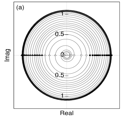
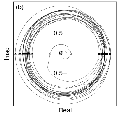
FIG. 5.: Typical eigenvalue curves in the complex plane. Plotted are the curves that two typical eigenvalues follow as the classicity ($1/\hbar$) is scanned. The eigenvalues remain near the origin until the classicity reaches a certain threshold (which is different for different eigenvalues of $T$), at which time they begin to spiral out to the unit circle. After that point, each time they cross the positive or negative real axis, Bogomolny’s theory predicts that the quantum system should have an even or odd parity eigenstate, respectively. Energies are: (a) $E=0.004$; (b) $E=0.2$. In each case, the fourth $T$-operator eigenvalue to move from the origin to the unit circle is plotted.

In order to see the behavior of the eigenvalues as the classicity is varied, it is necessary to “unroll” the curves. Figure 6 does this, showing the magnitudes of all of the eigenvalues, as a function of classicity.

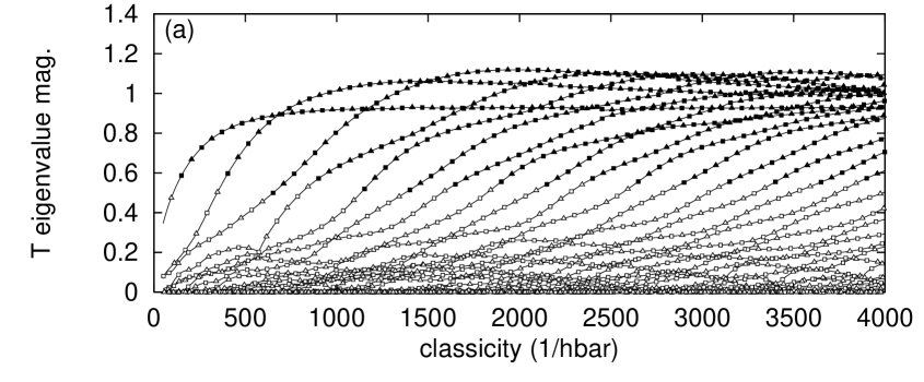
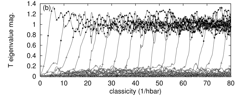
FIG. 6.: Magnitudes of the $T$-matrix eigenvalues as a function of $1/\hbar$. As the classicity is increased, eigenvalues move, one by one, from the origin towards the unit circle. Squares are plotted at those points where the eigenvalues have phases of $0$ (candidates to be even parity eigenstates), triangles at phase $\pi$ (odd eigenstates). The symbols are plotted solid for those candidates which turn out to be associated with true eigenstates of the quantum system (“Class 1” eigenvalues), and open for all others (“Class 0” eigenvalues). (a) $E=0.004$, which is in the classically regular regime. (b) $E=0.2$, which is in the classically chaotic regime. The horizontal axes are scaled such that the Thomas-Fermi densities of states in the horizontal directions are equal for the two energies. The plots predict the first 574 and 572 eigenstates, respectively, of the full quantum mechanical system.

At any choice of parameters, $T$ has two relatively well-defined classes of eigenvalues: those near the unit circle in the complex plane and those near the origin. In the following discussion we denote them as “Class 1” and “Class 0” eigenvalues, respectively. The separation of eigenvalues into these classes turns out to be an important feature of Bogomolny’s method, and will be discussed in detail below.

The general behavior of the eigenvalues is as follows: at very low classicity, all of the eigenvalues are located in a cloud near the origin (in Class 0). As the classicity is increased (corresponding to higher excitations of the quantum system), they spiral out, one by one, from the origin to an annulus near the unit circle (in Class 1). Thereafter, they remain near the unit circle, continuing to rotate counterclockwise. The behavior of the eigenvalues can be seen in Fig. 5.

1 The unitarity and dimension of $T$

Bogomolny shows that, in the limit $\hbar\rightarrow 0$ and for $y$ and $y^{\prime}$ on the classically allowed part of the surface of section, $T$ is unitary in the sense that $\langle y^{\prime}|T^{\dagger}T|y\rangle=\delta(y^{\prime}-y)$. The dimension of the “unitary part” of $T$, however, is finite, and is given by Eq. (4). When Eq. (4) is evaluated for the Nelson₂ potential, it gives the prediction that

$$\dim T=E\cdot(1/\hbar)\;.$$ (22)

To the extent that the eigenvalues separate into classes as mentioned above, then, the number of Class 1 eigenvalues at any given value of parameters is given by Eq. (22). This prediction is tested in Fig. 7—the staircase functions are a count of the number of eigenvalues that have migrated to Class 1 (more precisely, what is plotted is the number of eigenvalues that have predicted a quantum eigenstate).

FIG. 7.: Two notions of the dimension of the unitary part of the desymmetrized $T$ operator are plotted as a function of classicity, for (a) $E=0.004$, (b) $E=0.2$. The staircase is a count of how many of the eigenvalues have predicted a quantum eigenstate up to that point (roughly, the number of eigenvalues near the unit circle). The solid curve shows ${\rm Tr}\,T^{\dagger}T$, which is a continuous measure of the dimension of $T$. The dashed line shows Bogomolny’s theoretical prediction (Eq. (22)).

This doesn’t mean, however, that the $T$ matrix needs to be computed in a basis of this size, which would require a manual truncation. Rather, $T$ can be computed in a basis of arbitrarily large size, and the number of Class 1 eigenvalues will obey Eq. (22) automatically. The rest of the eigenvalues—an infinite number of them—remain in a cloud near the origin in Class 0, where they do not affect the subsequent predictions. Correspondingly, a different, continuous measure of the dimension of $T$ can be defined which does not require a truncation or a counting of Class 1 eigenvalues:

$$\dim T\equiv{\rm Tr}\,T^{\dagger}T\;.$$ (23)

This expression can be applied to computed $T$ matrices, and it reflects the fact that the dimension varies continuously with classicity. This measure is also plotted in Fig. 7. As can be seen, the agreement is quite good, even for low classicities. It is also noteworthy that the dimension varies even more smoothly than the curves of the individual eigenvalue magnitudes (Fig. 6); this is because variations in the magnitude of one eigenvalue tend to be negatively correlated with variations in those of another.

2 Finding the quantum spectrum from $T$ eigenvalues

Recall that the criterion for an even eigenstate of the system is that $T$ have an eigenvalue equal to $1$ (for brevity we temporarily ignore the odd-parity eigenstates that occur at eigenvalues of $-1$). Of course, Bogomolny’s method is a semiclassical approximation, which always entails the use of a stationary phase approximation to the exact Feynman path integral. Thus we shouldn’t be surprised that although the eigenvalues come near $1$, they never exactly equal $1$. Therefore, a more robust criterion is needed than “equality to 1.”

What is clear is that quantum eigenstates should only be associated with Class 1 eigenvalues—the eigenvalues that have magnitudes of approximately unity. As the classicity is increased, these eigenvalues rotate counterclockwise along the unit circle. On each rotation they pass close to 1 and “generate” an eigenstate. Leaving for later the subtleties of determining exactly which eigenvalues are in Class 1 and which are Class 0, we still need to decide at exactly which point during the rotation of a Class 1 eigenvalue the eigenstate is predicted to occur. At least three possible criteria suggest themselves:

1. the point at which $\det(1-T)=0$ is most nearly fulfilled;

2. the point where a Class 1 eigenvalue closest approaches $1$; and

3. the point where a Class 1 eigenvalue crosses the positive real axis (has a phase of $0$).

Although criterion 1 is the one emphasized by Bogomolny, it turns out to be unsatisfactory. The determinant mixes together information about all of the eigenvalues of $T$, whereas eigenstates are each associated with a single eigenvalue of $T$. Therefore, the minima that are supposed to indicate eigenstates are sometimes obscured, sometimes overlapping (and therefore indistinguishable), and often not very close to zero. Figure 8 shows all of these effects.

FIG. 8.: $|\det(1-T)|$ versus classicity. The determinant of $(1-T)$ is supposed to equal zero whenever the quantum mechanical system has an even eigenstate. Since the determinant is complex, we plot its magnitude as a function of classicity (the solid line) and indicate the exact eigenvalues with vertical dashed lines. Shown are: the lowest 19 even eigenstates for (a) $E=0.004$, (b) $E=0.2$; and about 25 eigenstates around the 275th even eigenstate for (c) $E=0.004$, (d) $E=0.2$. Although the minima match up reasonably well for the low-lying states, there is clearly little predictive power in the semiclassical determinant for highly-excited states. We shall see that monitoring individual eigenvalues of $T$ works better.

For the low-lying states, the minima do correlate reasonably well with the eigenstates of the quantum system, though there are already a few exceptions. However, for the highly excited states (here around $n=275$), the association is dramatically degraded. There is clearly little hope of making unambiguous predictions (let alone accurate ones) of highly-excited eigenstates of the quantum system based on a plot of $|\det(1-T)|$.

Criteria 2 and 3 produce results that differ only very slightly from one another. Criterion 3 is more robust than 2 and, we believe, more appropriate; therefore in our search for even parity eigenstates, we concentrate on those points where the $T$ operator has a Class 1 eigenvalue with $\text{\em phase}=0$. (Odd eigenstates are similarly found where a Class 1 eigenvalue has $\text{\em phase}=\pi$.) Accordingly, in Fig. 6 we have placed symbols on the curves whenever the eigenvalue crosses the real axis: squares and triangles mark the points where the eigenvalues have phases of $0$ or $\pi$, and which are thus candidates to be even or odd eigenstates, respectively.

It is important to emphasize that there is no ambiguity at all in the recipe for finding places where an eigenvalue crosses the real axis. Through the course of our numerical explorations, we found that the eigenvalues’ phases increase monotonically as the classicity was increased, except for a very few, brief exceptions. Since $T$ can be computed and diagonalized at any value of classicity, this means that any simple scheme suitable for finding a bracketed zero of a continuous function suffices to pinpoint the classicity at which a $T$ operator eigenvalue crosses the real axis of the complex plane.

Having now located all of the $\text{phase}=0$ points, it remains only to be determined exactly which of those candidates correspond to true quantum states. Equivalently, what we need is a criterion for sorting eigenvalues into Class 1 and Class 0. How close to $1$ do the eigenvalues need to be?

To investigate this question, we used our knowledge of the exact spectrum to determine which of the candidates matched true states. Thus a posteriori we were able to classify candidates accurately as Class 1 (corresponding to a true quantum state) or Class 0 (not associated with a quantum state). (In Fig. 6, the associated symbols are plotted solid if they are in Class 1, open if Class 0.) But more importantly, we would like to use our experience to describe how Class 1 eigenvalues could be distinguished from Class 0 eigenvalues a priori in a purely semiclassical calculation, without the benefit of knowing the exact answers.

The first criterion is, of course, the magnitude of the eigenvalue when it crosses the real axis. In the semiclassical limit, Class 1 eigenvalues are all supposed to have magnitude 1, and Class 0 eigenvalues, magnitude 0. At the finite classicity of our experiments, there is considerable deviation from that ideal, as shown in Fig. 9.

FIG. 9.: The separation of eigenvalues into Class 0 and Class 1. Plotted is the distribution of magnitudes of $T$ operator eigenvalues which cross the (positive or negative) real axis. The shaded part of the histogram contains Class 1 crossings, which are associated with true quantum eigenstates; the unshaded part, Class 0 crossings. (a) $E=0.004$. In this (regular) regime, there is a transition region around magnitude $0.5$, in which Class 0 and Class 1 eigenstates are both present and thus difficult to distinguish by magnitude alone. (b) $E=0.2$. In this (chaotic) regime, the two classes are well separated and Class 1 eigenvalues can easily be identified by their larger magnitudes. Note that in both cases, there are an infinite number of Class 0 crossings near zero magnitude.

While it is true that the eigenvalues tend to cluster around either the origin or the unit circle, the bands are pretty wide. Does the width of the bands cause practical problems?

In the regular regime, it sometimes does: there is a range of magnitudes, around 0.475–0.55, in which both Class 1 and Class 0 eigenvalues occur. In this overlap area, magnitude information is not sufficient to classify the eigenvalues. Fortunately, only a few percent of the eigenvalues fall into this uncertain range; the rest are predicted unambiguously by Bogomolny’s method. Even in this range, it is likely that in many cases one could tell which of the ambiguous eigenvalues need to be included in Class 1 by looking for deficits in the semiclassical staircase as compared to the Thomas-Fermi smoothed spectral staircase function, or deviations of the staircase dimension of $T$ (as in Fig. 7) from the semiclassically expected result.

In the chaotic regime, the width of the bands causes no problem: it is still easy to distinguish Class 1 from Class 0 eigenvalues, because of the large gap separating them. In our experiment in the chaotic regime, no Class 0 eigenvalues had magnitudes above 0.4, and no Class 1 eigenvalues had magnitudes below 0.65. This fortuitous circumstance is not only the result of the eigenvalues’ spiraling quickly from the origin to the unit circle; even a quick motion, if it occurred near a real-axis crossing, would cause trouble. The other important, and more surprising, property is that the eigenvalues all spiral out along a relatively narrow band in the lower complex half plane, and the entire journey is completed in less than the time it takes for half a rotation around the origin (see Fig. 10).

FIG. 10.: $T$-matrix eigenvalues in the complex plane, for $E=0.2$. This figure is similar to Fig. 5, except that all of the eigenvalues of $T$ are shown on the same plot. The striking feature revealed is that all of the eigenvalues spiral from the origin to the unit circle along a single band in the lower half of the complex plane. Within that rotation of $\pi$ radians, they manage to make it all the way from Class 0 to Class 1; during their brief transition, they are away from the real axis and so do not produce crossings of uncertain class.

As a result, there is no ambiguity whatsoever about the semiclassical method’s predictions for the location of eigenclassicities in the chaotic regime. This is so important and unexpected that it deserves to be emphasized: in the chaotic regime, Bogomolny’s method plus our criterion yield predictions of every single line in the quantum spectrum, with no spurious predictions whatsoever. This reliability is in contrast to that of other semiclassical methods, which frequently fail to resolve adjacent eigenstates and thereby leave doubt even about the number of eigenstates in a spectrum.

Altogether, the first 574 eigenstates in the regular regime, and the first 572 eigenstates in the chaotic regime (in each case, some even, some odd parity) are reproduced by the data. The accuracy of the semiclassical predictions will be discussed in Section IV D, after a few more qualitative observations.

3 Quantum numbers from the semiclassical data

Each Class 1 eigenvalue of the $T$ operator produces many eigenstates, one each time it rotates through the real axis. Consequently it is possible to separate the eigenstates into groups, based on which $T$ operator eigenvalue each one is associated with. In Fig. 6, eigenstates on a particular eigenvalue curve thus can be considered to be members of the same group. Although the groups are well defined in both regimes, they are truly meaningful only in the regular regime.

For the mostly regular energy $E=0.004$, the system is nearly an anisotropic harmonic oscillator, so it is nearly separable into $x$- and $y$-motions. Eigenstates of the system can therefore be labeled by two “almost good” quantum numbers, $n^{\prime}_{x}$ and $n^{\prime}_{y}$, which count the number of excitations along and perpendicular to the surface of section, respectively. The near separability is the reason that the eigenvalue curves in the regular regime are so smooth and unkinked; and the quantum numbers can be read off the picture as well. All of the eigenstates on the first eigenvalue curve have $n^{\prime}_{y}=0$—that is, they have no excitations in the vertical direction; those on the second curve have $n^{\prime}_{y}=1$; on the third curve, $n^{\prime}_{y}=2$; etc. Meanwhile $n^{\prime}_{x}$ can also be read off the diagram: the first eigenstate on a particular curve has $n^{\prime}_{x}=0$; the second, $n^{\prime}_{x}=1$; etc.

For the mostly chaotic energy $E=0.2$, however, the system is far from separable, and it has no set of good quantum numbers. The eigenstates still lie on continuous curves, but now the curves are kinked and bent whenever two eigenvalues approach each other in the complex plane. We see evidence that each interaction of two curves is accompanied by an intermixing of the eigenstates’ properties in the same manner as happens at “avoided crossings” of energy levels, seen when a quantum mechanical system’s external parameter is scanned adiabatically. So although the eigenstates are still connected by eigenvalue curves, the eigenstates lying on a single curve do not necessarily have similar properties, and the grouping by curves is not helpful.

D Accuracy of eigenclassicity spectra

We have now outlined all of the steps necessary to compute the eigenclassicity spectrum predicted by Bogomolny’s quantum surface of section method. In order to check its accuracy, it was necessary to decide, for each of the semiclassically computed eigenclassicities, which of the exact eigenclassicities it was “trying to predict.” This we did manually by comparing the two spectra; usually the eigenstates lined up so well that the correlation was obvious. When two states were very close to one another, the further step of comparing the exact and semiclassical surface of section wavefunctions was taken; this almost always made it obvious how to match up the numbers.

Figure 11 shows the errors of the semiclassical approximation as a function of classicity, for the two energy values.

FIG. 11.: Errors in the semiclassical eigenclassicity spectra. The discrepancy between the semiclassically predicted eigenclassicities and the exact values (obtained by diagonalizing the Hamiltonian), for (a) $E=0.004$ and (b) $E=0.2$. Squares represent even parity states; triangles, odd. In (a), lines connect eigenstates that are associated with a common eigenvalue of $T$ and which thus have in common the approximate quantum number $n^{\prime}_{y}$. Corresponding connections are not made in (b) because in this chaotic regime, associations of eigenstates do not form anything resembling continuous curves. The dashed curve shows the RMS error smoothed over small neighborhoods in classicity; note that it seems to remain roughly constant as the system becomes more classical.

Figs. 11(a) and 11(b) are scaled so as to be directly comparable to one another, in the sense that the vertical and horizontal axes are scaled in proportion to the respective Thomas-Fermi densities of state for the two energies. Each symbol on these plots represents an eigenclassicity predicted by Bogomolny’s method; its vertical position shows the amount by which the semiclassical prediction differed from the exact value. In Fig. 11(a), line segments connect eigenstates that are associated with the same $T$-matrix eigenvalue; this was not done in Fig. 11(b) for the reason mentioned at the end of the previous section (for that same reason, connecting them would not result in smooth curves, but rather in a tangled jumble).

We have already discussed some differences between the regular and the chaotic regimes—that when the system is classically chaotic it is somewhat more effort to calculate $T$, but somewhat less difficult to distinguish Class 1 from Class 0 eigenvalues—now we ask: how accurately does Bogomolny’s method predict eigenclassicities in the two regimes? From our numerical experiment it appears that the semiclassical method does not care about the degree of classical chaos; at least in this experiment, eigenstate positions are approximated by Bogomolny’s scheme just as well in the classically chaotic regime as in the classically regular regime.

Note also that the worst and RMS average errors seem to be roughly constant at all classicities—high excitation states’ positions are approximated just as well as low excitation states’. Moreover, when one follows individual curves in Fig. 11(a) (the nearly separable regime), one sees that individually the errors along any one curve seem to be decreasing towards zero. Remembering from Section IV C 3 that the eigenstates along a given curve share the same $n_{y}$ quantum number and have increasing $n_{x}$ quantum numbers, it seems that, at least in the regular regime, the semiclassical predictions are better for states which have more excitations transverse to the surface of section, but roughly constant regardless of the number of excitations along the SOS.

Why might this be? We suggest that it is a result of the method’s semi-semiclassical nature: the propogation of a wavefunction transverse to the surface of section is done semiclassically, and therefore improves when the number of excitations in that direction increases. The motion along the SOS, on the other hand, is effected (conceptually) by matrix multiplications, which are not dependent on the semiclassical approximation.

One can argue that efforts to find an analogous correlation (between errors and excitations along or perpendicular to the SOS) in the classically chaotic regime are doomed to failure because of the lack of even approximate quantum numbers. Not entirely satisfied by that argument, we sought such a correlation anyway, but so far without success.

The above comments refer to the absolute errors (in units of $1/\hbar$) of Bogomolny’s method in approximating the eigenclassicities of a quantum system. Figure 12 shows to what extent the method is able to meet a more exacting standard—the ability to resolve individual eigenstates.

FIG. 12.: Semiclassical errors in units of the mean level spacing. (a) $E=0.004$; (b) $E=0.2$. Alas, the rough constancy in the absolute errors demonstrated in Fig. 11 means that due to the increasing density of states of the quantum system, the semiclassical errors as a fraction of the mean level spacing, shown here, increase with increasing classicity, eventually preventing the resolution of individual eigenstates semiclassically. Nevertheless, after predicting nearly 600 eigenstates in each case, the worst semiclassical errors have yet to quite reach one mean level spacing, and the RMS averages (the dashed curves) less than half that.

There are theoretical reasons to believe that no semiclassical approximation which is correct only to first order in $\hbar$ will be able to resolve highly-excited eigenstates of a generic system with more than one degree of freedom: the density of states increases more quickly than the semiclassical approximation can hope to converge. The ability of a method to resolve individual eigenstates is measured by dividing its errors by the system’s mean level spacing. When this quantity approaches 1, nearby features of a spectrum can no longer be separated reliably.

Figure 12 shows this ratio for our system. The mean level spacing decreases like the reciprocal of the classicity, thereby “raising the standard” against which the approximations are judged. It is seen that Bogomolny’s method is a victim of the usual disease: the ratio of error to desymmetrized level spacing increases as the classicity is increased, so it will never be able to single out spectral features at very high excitation number. Still, its strain of the ailment is relatively nonvirulent—the worst error ratios are just creeping up towards 1 after hundreds of eigenstates have been predicted accurately.

E Calculating surface of section wavefunctions

The eigenstates of the $T$ operator are the values of the quantum mechanical wavefunction on the surface of section. That is, if

$\displaystyle\Psi(x,y)\equiv\langle x,y|\Psi\rangle$

is the 2-D quantum wavefunction, then to within a normalization,

$$\psi(y) \equiv \langle y|\psi\rangle$$

$$\propto \Psi(0,y)\;.$$

Odd parity surface of section eigenstates (which are zero on the SOS) can also be found—intuitively, by moving the surface of section an infinitesmal distance $\delta x$ from the $y$-axis:

$$\psi_{\text{odd}}(y) \propto \Psi(\delta x,y)$$

$$\propto \left.\frac{\partial\Psi(x,y)}{\partial x}\right|_{x=0}\;.$$

As usual, the eigenvalue problem only gives us the semiclassical wavefunctions to within a complex prefactor. Naturally we choose the magnitude of this prefactor to normalize the vector to 1, but there is still a complex phase that needs to be determined.

Since ideally, a phase could be chosen to make the SOS wavefunction pure real, it is sensible to choose the phase so as to minimize the imaginary part. Specifically, we try to minimize

$\displaystyle I\equiv\int dy\,[{\rm Im}\,\langle y|\psi\rangle]^{2}.$

Conveniently, this integral need never be done. Assuming that $|n\rangle$ is an orthogonal complete basis, and that $\langle y|n\rangle$ is always real, the required prefactor phase is simply

$$e^{i\phi}=\pm\sqrt{\frac{\sum_{n}\langle n|\psi\rangle^{2}}{|\sum_{n}\langle n|\psi\rangle^{2}|}}\;.$$ (24)

Since we store the SOS eigenfunctions in such a basis, only the sums appearing in (24) need to be done and no integrals. It turns out that after this best phase is chosen, the SOS wavefunctions indeed turn out to have only small imaginary parts.

A sequence of semiclassically predicted surface of section wavefunctions is plotted in Figs. 13 and 14, along with their exact counterparts. In each energy regime, 6 such plots are presented, at equivalent parts of their spectra (around the 230th eigenstate, which is about the 115th eigenstate of a particular parity). The eigenstates were not specially selected, and are typical of other eigenstates that we looked at. The three curves plotted in each set are: (1) the exact $\psi(y)^{2}$, which is necessarily real; (2) the semiclassically predicted $|\psi(y)|^{2}$; and (3) the square of the residual imaginary part of the semiclassically predicted wavefunction, $[{\rm Im}\,\psi(y)]^{2}$ (which ideally should be zero).

It can be seen from those figures that the semiclassical SOS wavefunctions capture, in almost all cases, the qualitative features of their exact counterparts. It is true that the semiclassical prediction is often rather poor at predicting the relative heights of peaks in the probability, but its estimate of oscillation length scales along the SOS are usually quite accurate. It can be seen that the semiclassical SOS wavefunctions are often too “sqeezed in” near the classical turning points, since they cannot model tunnelling. However, in many cases the details are predicted with surprising fidelity.

FIG. 13.: SOS eigenfunctions, regular regime. The eigenstates covered are the 6 starting at classicity $1/\hbar=2500$. (a) 115th even eigenstate: exact $1/\hbar=2506.08$; $\Delta(1/\hbar)=-0.39$. (b) 109th odd eigenstate: exact $1/\hbar=2508.20$; $\Delta(1/\hbar)=-1.69$. (c) 110th odd eigenstate: exact $1/\hbar=2511.33$; $\Delta(1/\hbar)=-2.38$. (d) 116th even eigenstate: exact $1/\hbar=2521.05$; $\Delta(1/\hbar)=-5.26$. (e) 111th odd eigenstate: exact $1/\hbar=2525.75$; $\Delta(1/\hbar)=-0.18$. (f) 112th odd eigenstate: exact $1/\hbar=2537.00$; $\Delta(1/\hbar)=-4.25$.

FIG. 14.: SOS eigenfunctions, chaotic regime. The eigenstates covered are the 6 starting at classicity $1/\hbar=50$. (a) 109th odd eigenstate: exact $1/\hbar=50.1654$; $\Delta(1/\hbar)=-0.0421$. (b) 114th even eigenstate: exact $1/\hbar=50.2430$; $\Delta(1/\hbar)=-0.0325$. (c) 110th odd eigenstate: exact $1/\hbar=50.2787$; $\Delta(1/\hbar)=-0.0060$. (d) 115th even eigenstate: exact $1/\hbar=50.3252$; $\Delta(1/\hbar)=-0.0526$. (e) 111th odd eigenstate: exact $1/\hbar=50.5255$; $\Delta(1/\hbar)=-0.0418$. (f) 116th even eigenstate: exact $1/\hbar=50.7136$; $\Delta(1/\hbar)=0.0534$.

V Conclusions

What is the point of a semiclassical theory? Historically, semiclassical theory came before, and inspired, matrix mechanics. However, in the intervening years, as the quantum method revealed its power and wide applicability, semiclassical methods barely inched forward. But finally in the late 1960’s and early 1970’s, two things happened. One was the (re-)discovery of chaos, and the realization that a big fraction of classical systems had been left unexplored and misunderstood, unknowingly assumed nonexistent by scientists whose training was virtually limited to ballistic trajectories, harmonic oscillators, and two-body Kepler problems. The second thing that happened was Gutzwiller’s discovery of his periodic orbit theory for semiclassical quantization. For the first time, semiclassical mechanics was liberated from the torus. The fashionable blending of these two developments, dubbed quantum chaos, is at its core nothing more than an attempt to understand semiclassical mechanics off the torus.

Gutzwiller’s trace formula is a beautiful edifice, so elegant that physicists have the gut feeling that it must be right. This makes it all the more frustrating that it is so hard to use. Periodic orbits are wonderful, canonically invariant objects that are easy to picture and describe. Unfortunately, very long period orbits in a typical chaotic potential are also furiously difficult to calculate. A speck of initial conditions, in a moderately to highly chaotic system, stretches into a gossamer hairball after only a few oscillations, and finding periodic orbits means finding places where the hairball and speck coincide—for all possible specks of initial conditions. A few such heroic computations have been done, and they are indeed able to reproduce the gross features of the quantum spectrum, and even individual low-lying states. However, as a practical method the trace formula has a long way to go.

It is not necessary to discard periodic orbit theory, but maybe it is time to expand our toolbox. It has been noted with admiration that periodic orbits, of longer and longer period, eventually densely explore every part of the phase space. Thus, it is argued, when we go to long enough orbits, the periodic orbits will “know” all there is to be known about the system’s classical mechanics. But this is vast overkill. We do not need to limit ourselves to periodic orbits if we want to explore all of phase space. Any set of trajectories—if sprinkled finely enough—does the job very nicely.

Bogomolny’s quantum surface of section method does just this. It democratically solicits the contributions of any and every trajectory. When the vote is over, periodic orbits still have disproportionate influence. But their influence comes incidentally, only because periodic orbits come with an entourage of similar behavior, non-periodic trajectories.

This paper presented an exploration of Bogomolny’s method. We explained how to apply this technique to an arbitrary potential in a practical way, and estimated just how efficient the method is when applied to systems of different dimension and different degrees of chaos. We suggested a practical and general way, by solving for eigenclassicities rather than eigenenergies, of testing this and other semiclassical theories with reduced effort. Then we used Bogomolny’s method to perform a semiclassical analysis of a generic, non-scalable, nonlinear oscillator, giving practical advice and techniques that will be useful to future users of the method. Our computation yielded hundreds of eigenvalue predictions in both the classically regular and the classically chaotic regimes, all accurate to less than a mean level spacing. We explored some of the properties of the $T$ operator, especially its dimension and the nature of its unitarity. Finally, we also computed the surface of section wavefunctions predicted by the method and found that they also agree quite well with their exact counterparts.

The hybrid nature of Bogomolny’s transfer operator—produced by summing classical trajectories, but then diagonalized using matrix methods—makes it something of a semi-semiclassical method. As such, it does not represent the yet-unattained “Holy Grail” of a purely semiclassical method which is able to resolve arbitrarily highly excited eigenenergies (indeed, it falls short on both counts). What this method is, however, is a practical method of semiclassically approximating information about quantum systems; a method which, though somewhat intricate to implement the first time, can function as a self-contained “black-box” that inputs Hamiltonians and outputs approximate quantum-mechanical spectra.

A Rescaling the Nelson₂ Potential

In this appendix, we discuss the rescaling of the “Nelson₂” potential that we use in the text, and its connection to the scaling for the true Nelson potential used by other authors (for example, [12]). We also discuss a different way of viewing the act of varying Planck’s constant (as was done in the main text in the form of the classicity): by adding an additional parameter and rescaling the dynamical variables, the same effect can be obtained while using a constant value for $\hbar$.

1 Connection to the “Nelson” potential

The system which has been given the name “Nelson” is defined by

$$\bar{H}={1\over 2}\bar{p}_{x}^{2}+{1\over 2}\bar{p}_{y}^{2}+{1\over 2}\bar{\mu}\bar{x}^{2}+\left(\bar{y}-{1\over 2}\bar{x}^{2}\right)^{2}$$ (A1)

Here, overbars are used to distinguish the variables in this scheme from our variables. For Nelson₂, the analogous equation is:

$$H={1\over 2}p_{x}^{2}+{1\over 2}p_{y}^{2}+{1\over 2}\omega^{2}x^{2}+{1\over 2}\left(y-{1\over 2}x^{2}\right)^{2}$$ (A2)

The only difference is the factor of ${1\over 2}$ preceding the nonlinear term in the new scaling, added as a minor convenience. The two sets of dynamical variables are related to one another by a simple scaling:

$$q_{x,y} = \bar{q}_{x,y}$$

$$p_{x,y} = {1\over\sqrt{2}}\bar{p}_{x,y}$$

$$H = {1\over 2}\bar{H}$$

$$\omega^{2} = {1\over 2}\bar{\mu}$$

$$t = \sqrt{2}\,\bar{t}$$

$$\hbar = {1\over\sqrt{2}}\bar{\hbar}$$

$$S = {1\over\sqrt{2}}\bar{S}$$

We should point out that our numerical experiments were done at a value of $\omega=\sqrt{0.05}$, which is equivalent to the choice $\bar{\mu}=0.1$ often used in Nelson potential analyses. Our selected energies $E=0.004$ and $E=0.2$ are equivalent to Nelson energies $\bar{E}=0.008$ and $\bar{E}=0.4$.

2 Making $\hbar$ constant again

As mentioned in the text, changing $\hbar$ (in the form of the classicity) is equivalent to a rescaling of the other dynamical variables. In the following we present the transformation which gives $\hbar$ back the constant value that Mother Nature intended (namely 1) by inserting a different parameter, $\tilde{\alpha}$, in the system. The equation which we now wish to compare to equation (A2) is as follows:

$$\tilde{H}={1\over 2}\tilde{p_{x}}^{2}+{1\over 2}\tilde{p_{y}}^{2}+{1\over 2}\tilde{\omega}^{2}\tilde{x}^{2}+{1\over 2}\left(\tilde{y}-{1\over 2}\tilde{\alpha}^{2}\tilde{x}^{2}\right)^{2}$$ (A3)

The other difference is that before, $\left[q_{x,y},p_{x,y}\right]=i\hbar$, whereas now, $\left[\tilde{q}_{x,y},\tilde{p}_{x,y}\right]=i$.

Again, a trivial scaling distinguishes the two schemes, so “changing” $\hbar$ is equivalent to scaling the other dynamical variables as follows:

$$\tilde{q}_{x,y} = q_{x,y}/\sqrt{\hbar}$$

$$\tilde{p}_{x,y} = p_{x,y}/\sqrt{\hbar}$$

$$\tilde{H} = H/\hbar$$

$$\tilde{\omega} = \omega$$

$$\tilde{t} = t$$

$$\tilde{\alpha} = \hbar$$

$$\tilde{\hbar} = 1$$

$$\tilde{S} = S/\hbar$$

REFERENCES

- [1] Author’s e-mail address: mhagger@krl.caltech.edu.
- [2] M. C. Gutzwiller, J. Math. Phys. 8, 1979 (1967).
- [3] M. C. Gutzwiller, J. Math. Phys. 10, 1004 (1969).
- [4] M. C. Gutzwiller, J. Math. Phys. 11, 1791 (1970).
- [5] M. C. Gutzwiller, J. Math. Phys. 12, 343 (1971).
- [6] E. B. Bogomolny, Nonlinearity 5, 805 (1992).
- [7] B. Lauritzen, Chaos 2, 409 (1992).
- [8] E. B. Bogomolny and M. Carioli, Physica D 67, 88 (1993).
- [9] T. Szeredi, J. H. Lefebvre, and D. A. Goodings, Phys. Rev. Lett. 71, 2891 (1993).
- [10] P. A. Boasman, Ph.D. thesis, University of Bristol (1992).
- [11] L. S. Schulman, J. Phys. A 27, 1703 (1994).
- [12] M. Baranger and K. T. R. Davies, Ann. Phys. (NY) 177, 330 (1987).
- [13] J. M. Robbins, Nonlinearity 4, 343 (1991).
- [14] B. Eckhardt and D. Wintgen, J. Phys. A: Math Gen. 24, 4335 (1991).
- [15] Unfortunately, although we used the first optimization, we did not notice the second one until our computations (in an oscillator basis) were finished, so updating the matrix was the most expensive part of the computational cost—though not prohibitively so.
- [16] D. Provost, Ph.D. thesis, Massachusetts Institute of Technology (1992).