LA-UR-94-2479

August 24, 1994

SEMIQUANTUM CHAOS AND

THE LARGE N EXPANSION

Fred Cooper^⋆, John Dawson^†, Salman Habib^⋆,

Yuval Kluger^⋆, Dawn Meredith^†, and Harvey Shepard^†

^⋆Theoretical Division and Center for Nonlinear Studies

Los Alamos National Laboratory

Los Alamos, NM 87545

^†Department of Physics

University of New Hampshire

Durham, NH 03824

Abstract

We consider the dynamical system consisting of a quantum degree of freedom $A$ interacting with $N$ quantum oscillators described by the Lagrangian

$$L={1\over 2}\dot{A}^{2}+\sum_{i=1}^{N}\left\{{1\over 2}\dot{x}_{i}^{2}-{1\over 2}(m^{2}+e^{2}A^{2})x_{i}^{2}\right\}~{}.$$ (1)

In the limit $N\rightarrow\infty$, with $e^{2}N$ fixed, the quantum fluctuations in $A$ are of order $1/N$. In this limit, the $x$ oscillators behave as harmonic oscillators with a time dependent mass determined by the solution of a semiclassical equation for the expectation value $\left\langle A(t)\right\rangle$. This system can be described, when $\left\langle x(t)\right\rangle=0$, by a classical Hamiltonian for the variables $G(t)=\left\langle x^{2}(t)\right\rangle$, $\dot{G}(t)$, $A_{c}(t)=\left\langle A(t)\right\rangle$, and $\dot{A_{c}}(t)$. The dynamics of this latter system turns out to be chaotic. We propose to study the nature of this large-$N$ limit by considering both the exact quantum system as well as by studying an expansion in powers of $1/N$ for the equations of motion using the closed time path formalism of quantum dynamics.

1 Introduction

The definition and observation of chaotic behavior in classical systems is familiar and more or less well understood [1]. However the proper definition of chaos for quantum systems and its experimental manifestations are still unclear [2]. Here we first study a simple model of two coupled systems which displays semiquantum chaos [3] when one of the systems can be treated “semiclassically.” We then study a purely quantum system of $N+1$ degrees of fredom which has the identical dynamics in the large $N$ limit as our original system. In this way we can determine, as a function of $N$, what is the time scale for quantum fluctuations of the “classical” oscillator to be of significant size. We also can determine how this time scale is related to the time scale determined by the maximum Lyapunov index. The question we are interested in here is whether quantum fluctuations become significant before or after the original system is sensitive to initial conditions.

In a classical chaotic system, such as the weather, we are accustomed to situations where there is lack of long time forecasting because of the sensitivity of the system to initial conditions. The simple model system considered here has the unusual feature that one has to give up long term forecasting even for the quantum mechanical probabilities, as exemplified by the average number of quanta at later times [3].

First let us review the original system which displayed semiquantum chaos. Consider two coupled quantum systems described by the Lagrangian,

$$L={1\over 2}\dot{x}^{2}+{1\over 2}\dot{A}^{2}-{1\over 2}(m^{2}+e^{2}A^{2})x^{2}~{}.$$ (2)

This Lagrangian leads to the Heisenberg equations of motion:

$$\ddot{x}+(m^{2}+e^{2}A^{2})x = 0$$ (3)

$$\ddot{A}+e^{2}x^{2}\,A = 0~{}.$$ (4)

The Hamiltonian is

$$H={1\over 2}p^{2}+{1\over 2}\Pi_{A}^{2}+{1\over 2}(m^{2}+e^{2}A^{2})x^{2}~{},$$ (5)

where $p(t)=\dot{x}(t)$ and $\Pi_{A}=\dot{A}(t)$. We next assume that we are in an experimental situation where the expectation value of $A(t)$ is so large that quantum fluctuations may be ignored. That is, we assume that $A$ is in a classical domain or in a coherent state (with large displacement). This is a particular assumption about approximating the expectation values involved in taking expectation values of the Heisenberg equations of motion, namely:

$$\left\langle A^{2}x\right\rangle=\left\langle A\right\rangle^{2}\left\langle x\right\rangle~{};~{}~{}\left\langle x^{2}A\right\rangle=\left\langle x^{2}\right\rangle\left\langle A\right\rangle$$ (6)

Here expectation value means taking a trace with respect to an initial density matrix defined at the initial time $t_{0}$, which we take to be $t_{0}=0$. Taking expectation values of the Heisenberg equations with the above factorization, we obtain

$$\left\langle\ddot{x}\right\rangle+(m^{2}+e^{2}\left\langle A\right\rangle^{2})\left\langle x\right\rangle = 0~{},$$ (7)

$$\left\langle\ddot{A}\right\rangle+e^{2}\left\langle x^{2}\right\rangle\left\langle A\right\rangle = 0~{}.$$ (8)

In this approximation, the equation for $\left\langle x\right\rangle$ is that of an harmonic oscillator with a time dependent mass, $m^{2}(t)=m^{2}+e^{2}\left\langle A\right\rangle^{2}$. $A$ can be thought of as a “classical” oscillator (since we do not include its quantum fluctuations) whose mass is determined by the quantum fluctuation of the $x$ oscillator (we consider the case where $\left\langle x\right\rangle$=0). The problem of a quantum harmonic oscillator with a time dependent mass can be solved in terms of the (numerical) solution of an auxiliary classical oscillator problem. We begin by noting that in the Heisenberg picture

$$[x(t),p(t)]=i~{}.$$ (9)

This commutation relation can be satisfied at all times by introducing time-independent (defined at $t=0$) creation and destruction operators, $a$ and $a^{\dagger}$, and using the Ansatz

$$x(t)=f(t)a+f^{*}(t)a^{\dagger}~{},$$ (10)

with $f(t)$ satisfying the Wronskian condition

$$i[f^{*}(t)\dot{f}(t)-\dot{f}^{*}(t)f(t)]=1~{}.$$ (11)

The destruction and creation operators $a$ and $a^{\dagger}$ satisfy the usual commutation relation $[a,a^{\dagger}]=1$. The commutation relation (9) then follows automatically.

It is easy to show using (3) and (10) that $f(t)$ satisfies the equation of motion

$$\ddot{f}+(m^{2}+e^{2}A^{2})f=0~{},$$ (12)

with the normalization fixed by the Wronskian condition (11). We can either solve this classical equation directly numerically, imposing the Wronskian condition at time $t=0$, or we can automatically impose the Wronskian condition by the substitution

$$f(t)={1\over\sqrt{2\Omega(t)}}\exp\left[-i\int_{0}^{t}\Omega(t^{\prime})dt^{\prime}\right]~{},$$ (13)

where $\Omega(t)$ satisfies the nonlinear differential equation

$${1\over 2}\left({\ddot{\Omega}\over\Omega}\right)-{3\over 4}\left({\dot{\Omega}\over\Omega}\right)^{2}+\Omega^{2}=\omega^{2}~{},$$ (14)

with

$$\omega^{2}(t)\equiv m^{2}+e^{2}A^{2}(t)~{}.$$ (15)

For simplicity we choose the initial state vector at $t=0$ to be the ground state of the operator $\hat{n}=a^{\dagger}a$, i.e., $|\Psi(0)\rangle=|0\rangle$, where $a|0\rangle=0$. Then, from (10), the average (classical) value of $x(t)$ and $p(t)$ is zero for all time, i.e., $\left\langle x(t)\right\rangle=0$ and $\left\langle p(t)\right\rangle=0$. This initial condition pertains in certain semiclassical time evolution problems, such as particle production by strong electromagnetic or gravitational fields. For the electric field problem, $A$ corresponds to the electric field, and $x$ to the $k=0$ mode of the charged particle field (See, e.g., Refs. [8][11]).

The quantum fluctuations of $x(t)$ are non-zero and are given by the variable $G(t)$,

$$G(t)=\left\langle x^{2}(t)\right\rangle=\left|f(t)\right|^{2}={1\over 2\Omega(t)}~{}.$$ (16)

From (14), it is easy to show that $G(t)$ satisfies

$${1\over 2}\left({\ddot{G}\over G}\right)-{1\over 4}\left({\dot{G}\over G}\right)^{2}-{1\over 4G^{2}}+\omega^{2}=0~{}.$$ (17)

In addition, we find that

$$\left\langle\dot{x}^{2}(t)\right\rangle={1\over 4}\left({\dot{G}^{2}\over G}+{1\over G}\right)~{}.$$ (18)

The expectation value of Eq. (5) becomes a new effective Hamiltonian

$$H_{eff} = \left\langle H(t)\right\rangle$$ (19)

$$= {1\over 2}\Pi_{A}^{2}+2\Pi_{G}^{2}G+{1\over 8G}+{1\over 2}(m^{2}+e^{2}A^{2})G~{}.$$

The momenta conjugate to $G$ and $A$ are

$$\Pi_{G}={\dot{G}\over 4G}~{},~{}~{}~{}~{}\Pi_{A}=\dot{A}~{}.$$ (20)

This classical Hamiltonian determines the variables, $G$ and $\dot{G}$, necessary for a complete quantum-mechanical description of the $x$ oscillator. Hamilton’s equations then yield

$$\dot{\Pi}_{G} = -2\Pi_{G}^{2}+{1\over 8G^{2}}-{1\over 2}\omega^{2}~{},$$

$$\dot{\Pi}_{A} = -e^{2}AG~{},$$ (21)

or equivalently,

$$\ddot{A}+e^{2}G\,A = 0~{},$$

$${1\over 2}\left({\ddot{G}\over G}\right)-{1\over 4}\left({\dot{G}\over G}\right)^{2}-{1\over 4G^{2}}+\omega^{2} = 0~{},$$ (22)

which correspond to (17) and the expectation value of Eq. (4).

The classical effective Lagrangian corresponding to the effective Hamiltonian (19) is

$$L_{eff}={1\over 2}{\dot{A}^{2}}+{1\over 8}\left({\dot{G}^{2}\over G}-{1\over G}\right)-{1\over 2}(m^{2}+e^{2}A^{2})G~{}.$$ (23)

This Lagrangian could also have been obtained using Dirac’s action,

$$\Gamma=\int dt\langle\Psi(t)|i{\partial\over\partial t}-H|\Psi(t)\rangle\equiv\int dt\,L_{eff},$$ (24)

and a time-dependent Gaussian trial wave function as described in Ref. [4]. This variational method has recently been used to study the quantum Henon-Heiles problem in a mean-field approximation [6]. In this method, the Gaussian trial wave function is parametrized as follows

$$\Psi(t)=[2\pi G(t)]^{-1/4}\exp[-(x-q(t))^{2}(G^{-1}(t)/4-i\Pi_{G}(t))+ip(t)(x-q(t))].$$ (25)

Here, $G(t)$ and $\Pi_{G}(t)$ are the time dependent real and imaginary parts of the width of the wave function. One can prove for our problem that if the quantum oscillator wave function starts at $t=0$ as a Gaussian, it is described at all times by the above expression, where $G(t)$ and $\Pi_{G}(t)$ are totally determined by solving the effective Hamiltonian dynamics. (For our special initial conditions $p(t)=q(t)=0$). Thus we find that our effective Hamiltonian totally determines the time evolution of the quantum oscillator.

One interesting “classical” variable is the expectation value of the time dependent adiabatic number operator, which corresponds to the number of quanta in a situation where the classical $A$ oscillator is changing slowly (adiabatically). For the related field theory problem of pair production of charged pairs by strong electric fields (where $A$ corresponds to the classical electromagnetic field and $x$ to the $k=0$ mode of the charged scalar field) this corresponds to the time dependent single particle distribution function of charged mesons. To find the expression for the number of quanta, which requires the definition of an adiabatic number operator, we begin with the wave function for the quantum oscillators corresponding to a slowly varying classical background $A$:

$$g(t)={1\over\sqrt{2\omega(t)}}\exp\left[-i\int_{0}^{t}\omega(t^{\prime})dt^{\prime}\right]$$ (26)

in terms of which we can decompose the quantum operator via

$$x(t)=g(t)b(t)+g^{\ast}(t)b^{\dagger}(t)~{}.$$ (27)

Requiring the momentum operator to have the form

$$p(t)=\dot{x}(t)=\dot{g}(t)b(t)+\dot{g}^{\ast}(t)b^{\dagger}(t)$$ (28)

by imposing $g(t)\dot{b}(t)+g^{\ast}(t)\dot{b}^{\dagger}(t)=0$, and recognizing that $g(t)$ and $g^{\ast}(t)$ satisfy the Wronskian condition by construction, one finds that $b(t)$ and $b^{\dagger}(t)$ have the usual interpretation as creation and annihilation operators, i.e., $[x(t),p(t)]=i$ and $[b(t),b^{\dagger}(t)]=1$. Note also that

$$b(t)=i[g^{\ast}(t)\dot{x}(t)-\dot{g}^{\ast}(t)x(t)]~{}.$$ (29)

It turns out that $b^{\dagger}(t)b(t)$ can be interpreted as a time-dependent number operator (assuming a slowly varying (adiabatic) classical field $A$). The time independent basis and the time dependent basis are both complete sets and are related by a unitary Bogoliubov transformation, $b(t)=\alpha(t)a+\beta(t)a^{\dagger}$, where

$$\alpha(t) = i[g^{\ast}(t)\dot{f}(t)-\dot{g}^{\ast}(t)f(t)]~{},$$ (30)

$$\beta(t) = i[g^{\ast}(t)\dot{f}^{\ast}(t)-\dot{g}^{\ast}(t)f^{\ast}(t)]~{},$$ (31)

and where $|\alpha(t)|^{2}-|\beta(t)|^{2}=1$. If we choose as initial conditions, $\Omega(0)=\omega(0)$, $\dot{\Omega}(0)=\dot{\omega}(0)$, then $\alpha(0)=1$ and $\beta(0)=0$. These are the initial conditions appropriate to the field theory problem of pair production. The average value of the time-dependent occupation number is given by

$$n(t)=\left\langle b^{\dagger}(t)b(t)\right\rangle=|\beta(t)|^{2}=(4\Omega\omega)^{-1}\left[(\Omega-\omega)^{2}+{1\over 4}\left({\dot{\Omega}\over\Omega}-{\dot{\omega}\over\omega}\right)^{2}\right]~{}.$$ (32)

Eq. (32) allows us to compute the average occupation number of the system as a function of time.

2 Numerical Solution of Hamilton’s equations

We now summarize some previous results from the numerical solution of the Hamiltonian equations obtained in the Gaussian approximation [3]. For calculational purposes, it turns out to be convenient to scale out the mass via the transformations $t\rightarrow m^{-1}t$, $A\rightarrow m^{-1/2}A$, $G\rightarrow m^{-1}G$, and $e\rightarrow em^{3/2}$. Then the scaled equations of motion are

$$\ddot{A}+e^{2}G\,A = 0$$

$${1\over 2}\left({\ddot{G}\over G}\right)-{1\over 4}\left({\dot{G}\over G}\right)^{2}-{1\over 4G^{2}}+1+e^{2}A^{2} = 0~{}.$$ (33)

In order to explore the degree of chaos as a function of (scaled) energy and coupling parameter $e$, we calculated surfaces of section and Lyapunov exponents. The surface of section is a slice through the three-dimensional energy shell [1]. That is, for a fixed energy and coupling parameter, the points on the surface of section are generated as the trajectory pierces a fixed place (e.g., $A=0$) in a fixed direction. The hallmark of regular motion is the cross section of a KAM torus which is seen as a closed curve in the surface of section. The hallmark of chaotic motion is the lack of any such pattern in the surface of section. In Fig. 1 we show a plot of a surface of section at $E=0.8$ and $e=1$ where regular and chaotic regions co-exist.

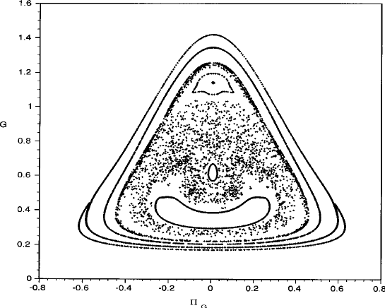
Figure 1: A plot of the surface of section for energy = $0.8$, $e=1.0$, and $A=0$. The one chaotic region is in the center of the plot.

The Lyapunov exponent provides a more quantitative, objective measure of the degree of chaos. The Lyapunov exponent, $\lambda$, gives the rate of exponential divergence of infinitesimally close trajectories [7]. Although there are as many Lyapunov exponents as degrees of freedom, it is common to simply give the largest of these. For regular trajectories $\lambda=0$; for chaotic trajectories the exponent is positive. To define the notion of a Lyapunov exponent one begins by considering the infinitesimal deviation from a fiducial trajectory,

$${\bf Z}(t)\equiv\lim_{\delta\rightarrow 0}{\bf z}({\bf z}_{0}+\delta,t)-{\bf z}({\bf z}_{0},t)~{},$$ (34)

where ${\bf z}({\bf z}_{0},t)$ is a point in phase space at time $t$ with initial position ${\bf z}_{0}$. The time evolution for ${\bf Z}(t)$ is given by

$${\dot{\bf Z}}(t)={\bf\nabla}{\bf F}\mid_{{\bf z}({\bf z}_{0},t)}\cdot{\bf Z}(t)~{},$$ (35)

where

$${\dot{\bf z}}(t)={\bf F}({\bf z}(t),t)$$ (36)

are the full equations of motion for the system. The (largest) Lyapunov exponent is defined to be

$$\lambda\equiv\lim_{t\rightarrow\infty}{1\over t}\ln\left|{{\bf Z}(t)\over{\bf Z}(0)}\right|~{}.$$ (37)

Appendix A of Ref. [7] provides an explicit algorithm for the calculation of all the Lyapunov exponents. Since we cannot carry out the $t\rightarrow\infty$ limit computationally, the regular trajectories are those for which $\lambda(t)$ decreases as $1/t$, while the chaotic trajectories give rise to $\lambda(t)$ that is roughly constant in time, as judged by a linear least-squares fit of $\log[\lambda(t)]$ vs. $\log(t)$.

We computed the Lyapunov exponents for three values of the scaled coupling constant $e$ ($0.1$, $1.0$, $10.0$) and for energies from $0.5$ to $2.0$. $E=0.5$ is the lowest energy possible, corresponding to the zero point energy of the oscillator; there is no upper limit on $E$. Fifty initial conditions were chosen at random for each energy bin of width $0.1$ and coupling parameter. One relevant quantity to study is the chaotic volume, the fraction of initial conditions with positive definite Lyapunov exponents (corresponding to chaotic behavior). Errors in this quantity arise because of the finite number of initial conditions chosen, and because the distinction between zero and positive exponents cannot be made with certainty at finite times. We found that for $e=0.1$, more than $95\%$ of trajectories were regular for all energies tested; for $e=1.0$ and $10.0$, there is a steadily increasing fraction of chaotic orbits between $0.5\leq E\leq 1.25$. For $1.25\leq E\leq 2.0$, more than $90\%$ of these orbits are chaotic. In Fig. 2 we show that the occupation number is sensitive to initial conditions.

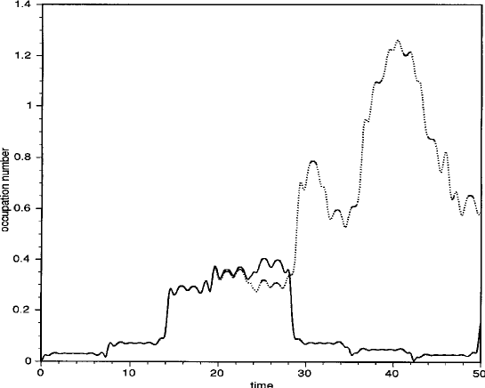
Figure 2: A plot of the occupation number given by Eq. (32) for energy =  $1.8$, $e=1.0$, $A(0)=0$, $\Pi_{G}(0)=0$. The solid line is for for $G(0)=0.5$; the dashed line is for $G(0)=0.5001$. This plot shows the sensitivity to initial conditions.

3 Quantum Oscillators and the Large-N Expansion

3.1 The Large-N Expansion and Semiquantum Chaos

In this section we show that the previous system of equations for the equations of motion for two oscillators are just the first term in a large-$N$ expansion for expectation values of the operator equations of motion of a quantum system consisting of $N$ copies of the original $x$ oscillator ($x\rightarrow x_{i},i=1,2,...,N$) and a single quantum dynamical variable $A$. Such a system is described by the operator equations of motion:

$$\ddot{x}_{i}+(m^{2}+e^{2}A^{2}(t))x_{i} = 0~{},$$

$$\ddot{A}+e^{2}\left(\sum_{i=1}^{N}x_{i}^{2}(t)\right)A = 0~{}.$$ (38)

If all the $N$ quantum oscillators $x_{i}$ have the same initial conditions then, at the level of expectation values, we can set all of them equal ($\left\langle x_{i}\right\rangle\equiv\left\langle x\right\rangle$) and obtain equations of motion for the expectation values:

$$\left\langle\ddot{x}\right\rangle+m^{2}\left\langle x\right\rangle+e^{2}\left\langle A^{2}(t)x\right\rangle = 0~{},$$

$$\left\langle\ddot{A}\right\rangle+e^{2}N\left\langle x^{2}(t)A\right\rangle = 0~{}.$$ (39)

We are interested in initial conditions where $\left\langle x\right\rangle=0$. In the large N limit we will show that in this case

$$\left\langle x^{2}A\right\rangle=\left\langle x^{2}\right\rangle\left\langle A\right\rangle+O(1/N)~{};~{}~{}~{}~{}\left\langle A^{2}x\right\rangle=\left\langle A\right\rangle^{2}\left\langle x\right\rangle+O(1/N),$$ (40)

so that after the rescaling,

$$A\rightarrow\sqrt{N}\tilde{A}~{};~{}~{}~{}~{}e^{2}\rightarrow\tilde{e}^{2}/N~{},$$ (41)

we recover the equations for the expectation values $\left\langle x^{2}\right\rangle=G(t)$ and $\left\langle\tilde{A}\right\rangle$ that pertained to semiquantum chaos. To compare with the orginal system describing semiquantum chaos we must solve the quantum system at different $N$ for fixed $\tilde{e}$. This value of $\tilde{e}$ must then be set equal to the value of $e$ used in the semiquantum chaos problem. We must also compare $\left\langle\tilde{A}(t)\right\rangle$ to the classical oscillator motion $A(t)$ to see the effects of the quantum fluctuations.

The exact quantum problem for the coupled quantum oscillators $x$ and $A$ can be studied as a function of $N$ once we supply the initial wave function at time $t=0$. Since we are interested in a comparison with our previous calculation, where $\tilde{e}$ is kept fixed, it is convenient to write the equations of motion as

$$\left\langle\ddot{x}\right\rangle+m^{2}\left\langle x\right\rangle+\tilde{e}^{2}\left\langle{A^{2}(t)\over N}x\right\rangle = 0~{},$$

$$\left\langle\ddot{A}\right\rangle+\tilde{e}^{2}\left\langle x^{2}(t)A\right\rangle = 0~{}.$$ (42)

The initial conditions, as we change N, are that for fixed $\tilde{A}_{0}(0)$ at time $t=0$,

$$\left\langle A(0)\right\rangle=\sqrt{N}\tilde{A}_{0}(0)~{};~{}~{}~{}~{}\left\langle x(0)\right\rangle=0~{}.$$ (43)

In the Schrödinger picture we have instead the time dependent Schrödinger equation

$$i{\partial\Psi(x_{i},A,t)\over\partial t}=\left[-{1\over 2}\sum_{i}{\partial^{2}\over\partial x_{i}^{2}}-{1\over 2}{\partial^{2}\over\partial A^{2}}+(m^{2}+e^{2}A^{2})\sum_{i}x_{i}^{2}\right]\Psi(x_{i},A,t)~{}.$$ (44)

With an eye to convenience in solving the Schrödinger equation we will choose an initial wave function which is a Gaussian in $A$ and $x$, so that the initial expectation values of $A$ and $x$ will be the ones specified above. This can be implemented by the initial wave function:

$$\Psi(t=0)=\prod_{i=1}^{N}\Psi_{x_{i}}(t=0)\Psi_{A}(t=0)~{},$$ (45)

$$\Psi_{A}(0)=[2\pi D(0)]^{-1/4}\exp[-(A-\sqrt{N}\tilde{A}_{0})^{2}(D^{-1}(0)/4-i\Pi_{D}(0))+ip_{A}(0)(A-\sqrt{N}\tilde{A}_{0})]~{}.$$ (46)

with

$$D(0)+N\tilde{A}_{0}^{2}=\left\langle A^{2}\right\rangle_{t=0}~{},~{}~{}~{}~{}\Pi_{D}(0)={\dot{D}(0)\over 4D(0)}~{},~{}~{}~{}~{}p_{A}(0)=\left\langle-i{\partial\over\partial A}\right\rangle_{t=0}~{},$$ (47)

and

$$\Psi_{x_{i}}(0)=[2\pi G(0)]^{-1/4}\exp\left[-x_{i}^{2}(G^{-1}(0)/4-i\Pi_{G}(0))\right]~{}.$$ (48)

These initial conditions can be used to compare, as a function of $N$, the exact quantum problem with the semiquantum chaos problem as well as the $1/N$ correction to the semiquantum chaos problem.

The large-$N$ expansion is best formulated using path integral methods for the generating function of the expectation values. For initial value problems rather special boundary conditions must be placed on the Green’s functions to insure causality. The formalism for doing this is the the closed time path (CTP) formulation of the effective action [9]. The marrying of the large $N$ expansion to the CTP formalism was accomplished recently, as described in Ref. [11].

Let us first ignore the issue of boundary conditions on the Green’s functions and discuss the generating functional for the expectation values. To obtain the generating functional we add sources to the original Lagrangian and consider the action

$$S=\int_{c}~{}L~{}dt$$ (49)

where the Lagrangian is,

$$L={1\over 2}\dot{A}^{2}+\sum_{i=1}^{N}\left\{{1\over 2}\dot{x}_{i}^{2}-{1\over 2}(m^{2}+e^{2}A^{2})x_{i}^{2}+j_{i}x_{i}\right\}+JA~{}.$$ (50)

The contour $c$ will be chosen in a way that enforces the correct boundary conditions for taking expectation values of operators at an initial time $t=0$. This will be discussed in the appendix.

The generating functional for the expectation values is given by the path integral:

$$Z[J,j]=\int{\rm d}[A]\int{\rm d}[x_{1}]\ldots\int{\rm d}[x_{N}]\>e^{iS[A,x;J,j]}~{}.$$ (51)

Since (50) is quadratic in the $x_{i}$ variables, we may integrate over all of them in (51) and obtain an effective action, given by:

$$Z[J,j]=\int{\rm d}[A]e^{iS_{eff}[A;J,j]}$$ (52)

where

$$S_{eff}[A;J,j] = \int_{c}dt\left\{-{1\over 2}A{{\rm d}^{2}A\over{\rm d}t^{2}}+JA\right\}+{iN\over 2}{\rm Tr~{}\ln}[G^{-1}(A)]$$ (53)

$${}+{1\over 2}\int_{c}dt\int_{c}dt^{\prime}\sum_{i}\left\{j_{i}(t)G(t,t^{\prime})j_{i}(t^{\prime})\right\}~{}.$$

Here, we have defined

$$G_{0}^{-1}(t,t^{\prime};A)=\left\{{{\rm d}^{2}\over{\rm d}t^{2}}+(m^{2}+e^{2}A^{2})\right\}\delta(t-t^{\prime})~{}.$$ (54)

Thus the Green’s function $G_{0}(t,t^{\prime})$ obeys

$$\left\{{{\rm d}^{2}\over{\rm d}t^{2}}+(m^{2}+e^{2}A^{2})\right\}G_{0}(t,t^{\prime\prime})=\delta(t-t^{\prime\prime})~{}.$$ (55)

The boundary conditions on this Green’s function needed to insure causality will be discussed later. We now consider the particular situation with all the $x_{i}$ identical (i.e., have identical initial conditions) so that $j_{i}=j,~{}x_{i}=x$. We also rescale $A$, $J$ and $e$ as follows:

$$\tilde{A} = A/\sqrt{N}$$

$$\tilde{J} = J/\sqrt{N}$$

$$\tilde{e} = e\sqrt{N}~{}.$$ (56)

The effective interaction now becomes proportional to $N$ as long as $\tilde{e}^{2}$ is kept fixed when $N$ is changed. This allows the evaluation of the remaining path integral over $A$ by the method of steepest descent and leads to an expansion of the expectation values as a power series in $1/N$. The value of the path integral at the stationary point is the leading term in this expansion, and the Gaussian fluctuations about the stationary point give the $1/N$ correction. Expanding the effective action about the stationary point:

$$S_{eff}[A;J,j] = S_{eff}[A_{0};J,j]$$ (57)

$$+\int_{c}dt^{\prime}\left[{\delta S_{eff}\over\delta A(t^{\prime})}\right]_{A_{0}}\left(A(t^{\prime})-A_{0}(t^{\prime})\right)$$

$$+\int_{c}dt^{\prime}\int_{c}dt^{\prime\prime}\left[{\delta^{2}S_{eff}\over\delta A(t^{\prime})\delta A(t^{\prime\prime})}\right]_{A_{0}}\left(A(t^{\prime})-A_{0}(t^{\prime})\right)\left(A(t^{\prime\prime})-A_{0}(t^{\prime\prime})\right)$$

$$+\cdots$$

The field $A_{0}$ is determined by the requirement

$$\left[{\delta S_{eff}\over\delta A(t)}\right]_{A_{0}}=0~{},$$ (58)

and setting,

$$D^{-1}_{0}(t,t^{\prime})=-\left[{\delta^{2}S_{eff}\over\delta A(t)\delta A(t^{\prime})}\right]_{A_{0}}~{},$$ (59)

the path integral in Eq. (53), including terms up to $1/N$, is given by

$$Z[J,j] = e^{iW[J,j]}$$

$$W[J,j] = S_{eff}[A_{0};J,j]+{i\over 2}{\rm Tr}\ln[D^{-1}_{0}(x_{0},A_{0})]+\cdots~{}.$$ (60)

Since the first term in the action is proportional to $N$ and the Gaussian fluctuation contribution is of order $N^{0}$, the fluctuation term gives the $1/N$ corrections. An auxiliary quantity which allows the direct determination of one particle irreducible vertices such as inverse Green’s functions is the effective action functional $\Gamma$ (not to be confused with $S_{eff}$) which is a Legendre transform of $W[J,j]$. Changing variables from $J,j$ to the expectation values $\left\langle x\right\rangle$, $\left\langle A\right\rangle$ where

$$\left\langle x\right\rangle\equiv\bar{x}={\delta W\over\delta j}~{};\hskip 14.45377pt\left\langle A\right\rangle\equiv\bar{A}={\delta W\over\delta J}~{}.$$ (61)

We now define the effective action functional (omitting the overline for symplicity of notation) as

$$\Gamma[x_{i},A]=W[j,J]-\int_{c}~{}dt~{}[j_{i}(t)x_{i}(t)+J(t)A(t)]~{},$$ (62)

which turns out to be, at order $1/N$,

$$\Gamma[x_{i},A]=S_{cl}[x_{i},A]+{iN\over 2}{\rm Tr}\,\ln[G^{-1}_{0}(A)]+{i\over 2}{\rm Tr}\,\ln[D^{-1}_{0}(x,A)]$$ (63)

where $S_{cl}$ is the classical action and where $A$ and $x$ are the expectation values of the Heisenberg operators accurate to order $1/N$.

We now demonstrate that at the stationary phase point the original problem is recovered. When the sources are set to zero,

$$\left[{\delta S_{eff}\over\delta A(t)}\right]_{A_{0}}=-\left\{{{\rm d}^{2}\over{\rm d}t^{2}}+e^{2}\left[\sum_{i}x_{0i}^{2}(t)+{N\over i}G_{0}(t,t;A_{0})\right]\right\}A_{0}(t)\equiv 0~{},$$ (64)

or after rescaling:

$$\left\{{{\rm d}^{2}\over{\rm d}t^{2}}+\tilde{e}^{2}\left[x_{0}^{2}(t)+{1\over i}G_{0}(t,t;A_{0})\right]\right\}\tilde{A}_{0}(t)=0~{},$$ (65)

where $G_{0}(t,t^{\prime};A_{0})$ satisfies

$$\left\{{{\rm d}^{2}\over{\rm d}t^{2}}+(m^{2}+e^{2}A_{0}^{2})\right\}G_{0}(t,t^{\prime};A_{0})=\delta(t-t^{\prime})~{},$$ (66)

and $x_{0i}(t)$ satisfies

$$\left\{{{\rm d}^{2}\over{\rm d}t^{2}}+(m^{2}+e^{2}A_{0}^{2})\right\}x_{0i}(t)=0~{}.$$ (67)

With the identification

$${1\over i}G_{0}(t,t)=G(t)$$ (68)

where $G(t)=\left\langle x^{2}(t)\right\rangle-\left\langle x(t)\right\rangle^{2}$, we arrive at the equations we studied earlier pertaining to semiquantum chaos. (For that problem we chose $\left\langle x(t)\right\rangle=0$.) Thus we have shown that the lowest order in $1/N$ solution to the problem displays semiquantum chaos (note that the quantity $e^{2}A^{2}$ is invariant under our rescaling).

In the above, the inverse propagator for the $A$ variable is given by:

$$D^{-1}_{0}(t,t^{\prime};A_{0})=-\left[{\delta^{2}S_{eff}\over\delta A(t)\delta A(t^{\prime})}\right]_{A_{0}}=d^{-1}_{0}(t,t^{\prime};A_{0})+\Pi^{\vphantom{-1}}_{0}(t,t^{\prime};A_{0})~{},$$ (69)

where

$$d^{-1}_{0}(t,t^{\prime};A_{0}) = \left\{{{\rm d}^{2}\over{\rm d}t^{2}}+e^{2}\left[\sum_{i}x_{0i}^{2}(t)+{N\over i}G_{0}(t,t;A_{0})\right]\right\}\delta(t-t^{\prime})~{},$$

$$\Pi_{0}(t,t^{\prime};A_{0}) = 2Ne^{4}A_{0}(t)\pi_{0}(t,t^{\prime};A_{0})A_{0}(t^{\prime})~{},$$

$$\pi_{0}(t,t^{\prime};A_{0}) = i\,G_{0}(t,t^{\prime};A_{0})\,G_{0}(t^{\prime},t;A_{0})-{2\over N}\sum_{i}x_{0i}(t)G_{0}(t,t^{\prime};A_{0})x_{0i}(t^{\prime})~{}.$$ (70)

Rescaling we have:

$$d^{-1}_{0}(t,t^{\prime};A_{0}) = \left\{{{\rm d}^{2}\over{\rm d}t^{2}}+\tilde{e}^{2}\left[x^{2}(t)+{1\over i}G_{0}(t,t;A_{0})\right]\right\}\delta(t-t^{\prime})~{},$$

$$\Pi_{0}(t,t^{\prime};A_{0}) = 2\tilde{e}^{4}\tilde{A}_{0}(t)\pi_{0}(t,t^{\prime};A_{0})\tilde{A}_{0}(t^{\prime})~{},$$

$$\pi_{0}(t,t^{\prime};A_{0}) = i\,G_{0}(t,t^{\prime};A_{0})G_{0}(t^{\prime},t;A_{0})-2x(t)G_{0}(t,t^{\prime};A_{0})x(t^{\prime})~{}.$$ (71)

We need to invert (69) subject to the correct causal boundary conditions to find $D_{0}(t_{1},t_{2};A_{0})$.

The causal Green’s function for initial value problems can be expressed in two ways, either as a two dimensional matrix Green’s function, or as a path ordered Green’s function defined on a complex contour. In this paper we will use the second method. As discussed in the appendix, the quantity that takes the place of the usual Feynman Green’s function is the causal Green’s function. We begin by defining an initial density matrix at time $t=0$ by $\rho$, and then introducing the two Wightman functions $G_{>}$ and $G_{<}$ via

$$G_{>}(t,t^{\prime}) = i\{\left\langle x(t)x(t^{\prime})\right\rangle-\left\langle x(t)\right\rangle\left\langle x(t^{\prime})\right\rangle\}$$

$$G_{<}(t,t^{\prime}) = i\{\left\langle x(t^{\prime})x(t)\right\rangle-\left\langle x(t^{\prime})\right\rangle\left\langle x(t)\right\rangle\}$$ (72)

where $\left\langle x(t)x(t^{\prime})\right\rangle\equiv Tr\{\rho x(t)x(t^{\prime})\}$. Time integrals are then defined on the contour shown in Fig. 3, with the integration path given by

$$\int_{c}dt=\int_{0:c_{+}}^{\infty}dt-\int_{0:c_{-}}^{\infty}dt~{}.$$ (73)

Figure 3: Complex time contour ${\cal C}$ for the closed time path propagators.

The causal Green’s functions which embody the correct boundary conditions are then

$$G(t,t^{\prime})=\Theta_{c}(t,t^{\prime})G_{>}(t,t^{\prime})+\Theta_{c}(t^{\prime},t)G_{<}(t,t^{\prime})~{},$$ (74)

where

$$\Theta_{c}(t,t^{\prime})=\cases{\Theta(t,t^{\prime})&for $t$ on $c_{+}$ and $t^{\prime}$ on $c_{+}$\cr 0&for $t$ on $c_{+}$ and $t^{\prime}$ on $c_{-}$\cr 1&for $t$ on $c_{-}$ and $t^{\prime}$ on $c_{+}$\cr\Theta(t^{\prime},t)&for $t$ on $c_{-}$ and $t^{\prime}$ on $c_{-}$}~{}.$$ (75)

The Green’s functions are symmetric and $A_{>}(t,t^{\prime})=A_{<}(t^{\prime},t)$. These propagators take the place of the usual Feynman ones for initial value problems. To calculate the $1/N$ corrections to the quantities $\left\langle A(t)\right\rangle$ and $\left\langle x(t)\right\rangle$ and $\left\langle x^{2}(t)\right\rangle$ one needs to take functional derivatives of the generating functional, all correct to order $1/N$. Specifically we have:

$$\left\langle A(t)\right\rangle={\delta W[J,j]\over\delta J(t)}$$ (76)

where $W[J,j]$ is given in Eq. (60).

To separate out the leading and next to leading order terms, we write,

$$\left\langle A(t)\right\rangle=A_{0}(t)+A_{1}(t)~{},$$ (77)

where $A_{0}(t)$ is the quantity determined in first order, by Eq. (65). $A_{1}(t)$ is given by

$$A_{1}(t)={i\over 2}\int_{c}dt^{\prime}\int_{c}dt_{1}\int_{c}dt_{2}D_{0}(t,t^{\prime};A_{0})\left({\delta D_{0}^{-1}(t_{1},t_{2};A_{0})\over\delta A_{0}(t^{\prime})}\right)D_{0}(t_{2},t_{1};A_{0})~{}.$$ (78)

By straightforward differentiation, it is possible to show that $A_{1}(t)$ gets contributions from three terms when $\left\langle x\right\rangle=0$. Namely,

$$A_{1}(t)=A_{1}^{(a)}(t)+A_{1}^{(b)}(t)+A_{1}^{(c)}(t)~{},$$ (79)

where

$$A_{1}^{(a)}(t) = {i\tilde{e}^{4}\over N}\int_{c}dt_{1}\int_{c}dt_{2}K^{(a)}(t,t_{2},t_{3})~{},$$

$$K^{(a)}(t,t_{2},t_{3}) = D_{0}(t,t_{2};A_{0})A_{0}(t_{2})\pi_{0}(t_{2},t_{3};A_{0})D_{0}(t_{3},t_{3};A_{0})~{},$$ (80)

$$A_{1}^{(b)}(t) = {2i\tilde{e}^{4}\over N}\int_{c}dt_{2}\int_{c}dt_{3}K^{(b)}(t,t_{2},t_{3})~{},$$

$$K^{(b)}(t,t_{2},t_{3}) = D_{0}(t,t_{2};A_{0})\pi_{0}(t_{2},t_{3};A_{0})D_{0}(t_{2},t_{3};A_{0})A_{0}(t_{3})~{},$$ (81)

$$A_{1}^{(c)}(t) = -{4i\tilde{e}^{6}\over N}\int_{c}dt_{2}\int_{c}dt_{3}\int_{c}dt_{4}K^{(c)}(t,t_{2},t_{3},t_{4})~{},$$

$$K^{(c)}(t,t_{2},t_{3},t_{4}) = D_{0}(t,t_{2};A_{0})\tilde{A}_{0}(t_{2})G_{0}(t_{2},t_{3};A_{0})\tilde{A}_{0}(t_{3})$$ (82)

$$\times G_{0}(t_{2},t_{4};A_{0})A_{0}(t_{4})\Sigma(t_{3},t_{4};A_{0})~{}.$$

In the above expressions, the self energy $\Sigma$ is given by

$$\Sigma(t_{3},t_{4};A_{0})=iD_{0}(t_{3},t_{4};A_{0})G_{0}(t_{3},t_{4};A_{0})~{},$$ (83)

and the polarization $\pi$ by

$$\pi(t_{3},t_{4};A_{0})=iG_{0}(t_{3},t_{4};A_{0})G_{0}(t_{3},t_{4};A_{0})~{}.$$ (84)

Note that the causal Green’s functions are symmetric under the interchange of time labels. It is easy to show, using the rules for convoluting the causal Green’s functions (given below), that $A_{1}(t)$ only depends on information from previous times.

In order to evaluate the above graphs we first have to determine the causal propagator $D_{0}$. From (69), we have

$$D^{-1}_{0}(t,t^{\prime})=d^{-1}_{0}(t,t^{\prime})+\Pi_{0}(t,t^{\prime})~{},$$ (85)

where $d^{-1}_{0}(t,t^{\prime})$ and $\Pi_{0}(t,t^{\prime})$ are defined in (70). The defining equations for the inverses are

$$\int_{c}dt^{\prime}\,d^{-1}_{0}(t,t^{\prime})d^{\vphantom{-1}}_{0}(t^{\prime},t^{\prime\prime}) = \delta(t-t^{\prime\prime})~{},$$

$$\int_{c}dt^{\prime}\,D^{-1}_{0}(t,t^{\prime})D^{\vphantom{-1}}_{0}(t^{\prime},t^{\prime\prime}) = \delta(t-t^{\prime\prime})~{}.$$ (86)

If we now put

$$D_{0}(t,t^{\prime})=d_{0}(t,t^{\prime})+\tilde{D}_{0}(t,t^{\prime})~{},$$ (87)

then (86) implies

$$\int_{c}dt^{\prime}\left\{d^{-1}_{0}(t,t^{\prime})+\Pi^{\vphantom{-1}}_{0}(t,t^{\prime})\right\}D^{\vphantom{-1}}_{0}(t^{\prime},t^{\prime\prime})=\delta(t-t^{\prime\prime})~{},$$ (88)

or

$$\int_{c}dt^{\prime}d^{-1}_{0}(t,t^{\prime})\tilde{D}^{\vphantom{-1}}_{0}(t,t^{\prime})=-\int_{c}{\rm d}t^{\prime}\,\Pi^{\vphantom{-1}}_{0}(t,t^{\prime})D^{\vphantom{-1}}_{0}(t^{\prime},t^{\prime\prime})~{}.$$ (89)

We can now invert the left hand side using (86) again, obtaining:

$$D_{0}(t_{1},t_{4})=d_{0}(t_{1},t_{4})-\int_{c}dt_{2}\int_{c}dt_{3}\,d_{0}(t_{1},t_{2})\Pi_{0}(t_{2},t_{3})D_{0}(t_{3},t_{4})~{}.$$ (90)

We use (90) to find the inverse. Note that $d_{0}(t,t^{\prime})$ satisfies

$$\left\{{{\rm d}^{2}\over{\rm d}t^{2}}+e^{2}\left[\sum_{i}x_{0i}^{2}(t)+{N\over i}G_{0}(t,t)\right]\right\}\,d_{0}(t,t^{\prime})=\delta(t-t^{\prime})~{}.$$ (91)

We will need to solve for this Green’s function $d_{0}$ in order to find $D_{0}(t,t^{\prime})$ from (90). As shown below this can be done in analogy to the determination of $G(t)$ in the semiquantum problem, that is, we will introduce a set of mode functions for an auxiliary quantum problem.

To study the time it takes for the $1/N$ corrections to become significant, we also need to determine the $1/N$ correction to the $x$ oscillator propagator. This is obtained once again by functional differentiation. Now we turn to the full Green’s function $\bar{G}(t,t^{\prime})$ for the $x$ oscillator (to order $1/N$), from which we can obtain

$$\left\langle x^{2}(t)\right\rangle={1\over i}\bar{G}(t,t).$$ (92)

This is most easily determined to order $1/N$ from the inverse Green’s function which by the chain rule is the negative of the second derivative of the effective action functional $\Gamma[x,A]$ with respect to $x$. The effective action functional $\Gamma$ to order $1/N$ is

$$\Gamma[x_{i},A]=S_{cl}[x_{i},A]+i{N\over 2}{\rm Tr}\ln[G^{-1}_{0}(A)]+{i\over 2}{\rm Tr}\ln[D^{-1}_{0}(x,A)]~{},$$ (93)

where $S_{cl}$ is the classical action and here $A$ and $x$ are the expectation values of the Heisenberg operators accurate to order $1/N$, i.e., the $A$ in this equation is the solution of $\delta\Gamma/\delta A=0$, or

$$\left\{{{\rm d}^{2}\over{\rm d}t^{2}}+e^{2}\left[\sum_{i}x_{0i}^{2}(t)+{N\over i}G_{0}(t,t;A)\right]\right\}\,A(t)={i\over 2}\int_{c}~{}dt_{1}\int_{c}~{}dt_{2}D_{0}(t_{1},t_{2};A){\delta D_{0}(t_{2},t_{1};A)\over\delta A(t)}\\$$ (94)

and differs from the stationary point $A_{0}$ of the original path integral by terms of order $1/N$. Now

$$\bar{G}^{-1}_{ij}(t,t^{\prime};A) = -{\delta^{2}\Gamma\over\delta x_{i}(t)\delta x_{j}(t^{\prime})}$$ (95)

$$= G_{0}^{-1}(t,t^{\prime};A)\delta_{ij}-{i\over 2}\int_{c}~{}dt_{1}\int_{c}~{}dt_{2}D_{0}(t_{1},t_{2};A){\delta^{2}D_{0}(t_{2},t_{1};A)\over\delta x_{i}(t)\delta x_{j}(t^{\prime})}$$

$$= \delta_{ij}\bar{G}^{-1}(t,t^{\prime};A)~{}.$$

And, since

$${\delta^{2}D_{0}(t_{2},t_{1};A)\over\delta x_{i}(t)\delta x_{j}(t^{\prime})} = 2e^{2}\delta(t_{1}-t_{2})\delta(t_{1}-t)\delta(t_{2}-t^{\prime})$$

$$- 4e^{4}A(t)G_{0}(t,t^{\prime};A)A(t^{\prime})[\delta(t_{1}-t)\delta(t_{2}-t^{\prime})+\delta(t_{1}-t^{\prime})\delta(t_{2}-t)]~{},$$

we obtain

$$\bar{G}^{-1}(t,t^{\prime};A)={G_{0}}^{-1}(t,t^{\prime};A)+\bar{G_{1}}^{-1}(t,t;A),$$ (97)

where $\bar{G_{1}}^{-1}$ is of order $1/N$ and given by two terms. Explicitly,

$$\bar{G_{1}}^{-1}(t,t^{\prime})=-i{\tilde{e}^{2}\over N}D_{0}(t,t)\delta(t-t^{\prime})+4{\tilde{e}^{4}\over N}\tilde{A}_{0}(t)\Sigma(t,t^{\prime})\tilde{A}_{0}(t^{\prime})~{}.$$ (98)

To obtain the $1/N$ expansion of $\bar{G}$ we have to invert this to order $1/N$. We first need to reexpand $G_{0}^{-1}(A)$ up to order $1/N$ since $A=A_{0}+A_{1}$ where $A_{1}$ is given by (78). We have,

$$\bar{G}^{-1}(t,t^{\prime}) = {G_{0}}^{-1}(A_{0})(t,t^{\prime})+2e^{2}A_{0}(t)A_{1}(t)\delta(t-t^{\prime})+\bar{G_{1}}^{-1}(t,t^{\prime})$$ (99)

$$\equiv {G_{0}}^{-1}(A_{0})(t,t^{\prime})+{1\over N}\Delta(t,t^{\prime})~{}.$$

Inverting to order $1/N$ we obtain finally

$$\bar{G}(t,t^{\prime})=G_{0}(t,t^{\prime};A_{0})-{1\over N}\int_{c}dt_{1}~{}\int_{c}dt_{2}~{}G_{0}(t,t_{1};A_{0})\Delta(t_{1},t_{2})G_{0}(t_{2},t^{\prime};A_{0})+O(1/N^{2})~{}.\\$$ (100)

3.2 Closed time path contour and causality

In this section we discuss the causality of the Green’s functions as given by the CTP formalism. We will evaluate the time integrals using the closed time path (CTP) contour shown in Fig. 3. The integration path is given explicitly by

$$\int_{c}dt=\int_{0:c_{+}}^{\infty}dt-\int_{0:c_{-}}^{\infty}dt~{}.$$ (101)

The Green’s functions are now given by functions of the form,

$$A(t,t^{\prime})=\Theta_{c}(t,t^{\prime})A_{>}(t,t^{\prime})+\Theta_{c}(t^{\prime},t)A_{<}(t,t^{\prime})~{},$$ (102)

where $\Theta_{c}(t,t^{\prime})$ is defined in Eq. (75). We call such functions causal. The causal Green’s functions are symmetric implying thereby that $A_{>}(t,t^{\prime})=A_{<}(t^{\prime},t)$. In order to prove causality of any particular graph we need to discuss two lemmas. The first is that if we have a loop of two causal functions, such as found in a self energy graph, then that is also a causal function. To show this one just needs the definition of $\Theta_{c}$. If the two causal functions are

$$B(t,t^{\prime}) = \Theta_{c}(t,t^{\prime})B_{>}(t,t^{\prime})+\Theta_{c}(t^{\prime},t)B_{<}(t,t^{\prime})~{},$$

$$C(t,t^{\prime}) = \Theta_{c}(t,t^{\prime})C_{>}(t,t^{\prime})+\Theta_{c}(t^{\prime},t)C_{<}(t,t^{\prime})~{},$$ (103)

then the self energy graph is also causal. Letting the self energy

$$A(t,t^{\prime})=iB(t,t^{\prime})C(t,t^{\prime})~{},$$ (104)

and setting,

$$A_{>,<}(t,t^{\prime})=iB_{>,<}(t,t^{\prime})C_{>,<}(t,t^{\prime})~{},$$ (105)

we find

$$A(t,t^{\prime})=\Theta_{c}(t,t^{\prime})A_{>}(t,t^{\prime})+\Theta_{c}(t^{\prime},t)A_{<}(t,t^{\prime})~{},$$ (106)

which is the desired result.

The next lemma is that the matrix product of two causal functions is causal. That is, if we think of the Green’s functions as matrices in time and if we matrix multiply B and C so that $A(t_{1},t_{3})$ is given by

$$A(t_{1},t_{3})=\int_{c}{\rm d}t_{2}\,B(t_{1},t_{2})C(t_{2},t_{3})~{},$$ (107)

we find then

$$A(t,t^{\prime})=\Theta_{c}(t,t^{\prime})A_{>}(t,t^{\prime})+\Theta_{c}(t^{\prime},t)A_{<}(t,t^{\prime})~{},$$ (108)

where

$$A_{\stackrel{{\scriptstyle>}}{{<}}}(t_{1},t_{3}) = -\int_{0}^{t_{3}}{\rm d}t_{2}B_{\stackrel{{\scriptstyle>}}{{<}}}(t_{1},t_{2})\left[C_{>}(t_{2},t_{3})-C_{<}(t_{2},t_{3})\right]$$ (109)

$$+\int_{0}^{t_{1}}{\rm d}t_{2}\left[B_{>}(t_{1},t_{2})-B_{<}(t_{1},t_{2})\right]C_{\stackrel{{\scriptstyle>}}{{<}}}(t_{2},t_{3})~{}.$$

This lemma is discussed in Ref. [11] and is obtained directly by breaking the time integration into three segments, viz.,

$$(i) 0<t_{i}<t,\ {\rm on}\ {\cal C}_{+}~{},$$ (110)

$$(ii) t<t_{i}<\infty,\ {\rm on}\ {\cal C}_{+}~{},$$

$$(iii) 0<t_{i}<\infty,\ {\rm on}\ {\cal C}_{-}~{}.$$

One then uses the definition of the $\Theta$ function (75) and collects all the non-cancelling terms.

Now consider the product of three causal functions:

$$A(t_{1},t_{4})=\int_{c}dt_{2}\int_{c}dt_{3}B(t_{1},t_{2})C(t_{2},t_{3})D(t_{3},t_{4})~{}.$$ (111)

We can work this case out by applying the second lemma from left to right. That is, we can let

$$E(t_{1},t_{3})=\int_{c}dt_{2}\,B(t_{1},t_{2})C(t_{2},t_{3})~{}.$$ (112)

Then $E(t_{1},t_{3})$ is causal and is given by an equation of the form (108). We are then left with an equation of the form:

$$A(t_{1},t_{4})=\int_{c}dt_{3}E(t_{1},t_{3})D(t_{3},t_{4})~{},$$ (113)

which is also causal. In the same way, we can find causal relations for any number of CTP integrals of causal functions. We can also apply the lemma from right to left. After doing the integrals sequentially one is eventually left with

$$f(t)=\int_{c}dt_{1}F(t,t_{1})=\int_{0}^{t}\left[F_{>}(t,t_{1})-F_{<}(t,t_{1})\right]~{},$$ (114)

which explicitly displays the causality.

3.3 Lowest order causal Green’s functions

With the results of the previous section in hand we are now in a position to solve for the Green’s functions with the correct causal structure. We would like to solve

$$\left\{{{\rm d}^{2}\over{\rm d}t^{2}}+(m^{2}+\tilde{e}^{2}\tilde{A}_{0}^{2}(t))\right\}G_{0}(t,t^{\prime}) = \delta(t-t^{\prime})~{},$$

$$\left\{{{\rm d}^{2}\over{\rm d}t^{2}}+\tilde{e}^{2}\left[x_{0}^{2}(t)+{1\over i}G_{0}(t,t)\right]\right\}d_{0}(t,t^{\prime}) = \delta(t-t^{\prime})~{},$$ (115)

subject to causal boundary conditions and an initial density matrix which is that of an adiabatic vacuum at time zero. The adiabatic requirement is satisfied by considering auxiliary quantum fluctuation operators $x_{0}$ and $A_{0q}$ such that $\left\langle x_{0}\right\rangle=\left\langle A_{0q}\right\rangle=0$. (Note that we are defining the fluctuation operators by writing the Heisenberg operator $A=\left\langle A\right\rangle+A_{q}$.) These operators are defined via

$$x_{0}^{\vphantom{\ast}}(t) = f(t)a+f^{\ast}(t)a^{\ast}$$

$$A_{0q}(t) = g(t)b+g^{\ast}(t)b^{\ast}~{},$$ (116)

where $a$ and $b$ are canonical annihilation (creation) operators satisfying

$$[a,a^{\dagger}]=[b,b^{\dagger}]=1~{},$$ (117)

and the adiabatic vacuum is defined by

$$a\left|0\right\rangle_{ad}=b\left|0\right\rangle_{ad}=0~{}.$$ (118)

The $f(t)$ and $g(t)$ are functions of time satisfying the homogeneous equations,

$$\left\{{{\rm d}^{2}\over{\rm d}t^{2}}+(m^{2}+\tilde{e}^{2}\tilde{A}_{0}^{2}(t))\right\}f(t) = 0$$

$$\left\{{{\rm d}^{2}\over{\rm d}t^{2}}+\tilde{e}^{2}\left[x_{0}^{2}(t)+{1\over i}G_{0}(t,t)\right]\right\}g(t) = 0~{},$$ (119)

with Wronskian conditions,

$$i\biggl{\{}f^{\ast}(t)\vbox{\halign{#\cr$\mathord{\leftarrow}\mkern-6.0mu\cleaders\hbox{$\mkern-2.0mu\mathord{-}\mkern-2.0mu$}\hfill\mkern-6.0mu\mathord{\rightarrow}$\crcr\kern-1.0pt\nointerlineskip\cr$\hfil\displaystyle{{{\rm d}\over{\rm d}t}}\hfil$\crcr}}f(t)\biggr{\}} = 1$$ (122)

$$i\biggl{\{}g^{\ast}(t)\vbox{\halign{#\cr$\mathord{\leftarrow}\mkern-6.0mu\cleaders\hbox{$\mkern-2.0mu\mathord{-}\mkern-2.0mu$}\hfill\mkern-6.0mu\mathord{\rightarrow}$\crcr\kern-1.0pt\nointerlineskip\cr$\hfil\displaystyle{{{\rm d}\over{\rm d}t}}\hfil$\crcr}}g(t)\biggr{\}} = 1~{}.$$ (125)

We can write the causal Green’s functions in terms of the complex functions $f(t)$ and $g(t)$,as follows:

$$G_{0}(t,t^{\prime}) = \Theta_{c}(t,t^{\prime})G_{0>}(t,t^{\prime})+\Theta_{c}(t^{\prime},t)G_{0<}(t,t^{\prime})$$

$$d_{0}(t,t^{\prime}) = \Theta_{c}(t,t^{\prime})d_{>}(t,t^{\prime})+\Theta_{c}(t^{\prime},t)d_{<}(t,t^{\prime})~{},$$ (126)

where

$$G_{0>}(t,t^{\prime}) = \left\langle x_{0}(t)x_{0}(t^{\prime})\right\rangle=if(t)f^{\ast}(t^{\prime})~{},$$ (127)

$$G_{0<}(t,t^{\prime}) = \left\langle x_{0}(t^{\prime})x_{0}(t)\right\rangle=if(t^{\prime})f^{\ast}(t)~{},$$ (128)

$$d_{>}(t,t^{\prime}) = \left\langle A_{0q}(t)A_{0q}(t^{\prime})\right\rangle=ig(t)g^{\ast}(t^{\prime})~{},$$ (129)

$$d_{<}(t,t^{\prime}) = \left\langle A_{0q}(t^{\prime})A_{0q}(t)\right\rangle=ig(t^{\prime})g^{\ast}(t)~{}.$$ (130)

Note also that

$$G_{0}(t,t) = i|f(t)|^{2}=iG(t)~{},$$

$$d_{0}(t,t) = i|g(t)|^{2}~{}.$$ (131)

Here the factors of $i$ are introduced to agree with earlier definitions. We are now in a position of being able to find the $1/N$ quantum corrections to $A_{1}(t)$ and $\left\langle x^{2}(t)\right\rangle$, using Eq. (90) to construct $D_{0}(t,t^{\prime})$. The last-named quantity obeys the integral equation

$$D_{0}(t_{1},t_{4})=d_{0}(t_{1},t_{4})-\int_{c}dt_{2}\int_{c}dt_{3}d_{0}(t_{1},t_{2})\Pi_{0}(t_{2},t_{3})D_{0}(t_{3},t_{4})~{}.$$ (132)

We want to evaluate this in terms of the lowest order quantities. The polarization can be put in causal form since

$$\pi_{0}(t,t^{\prime})=i[\Theta_{c}(t,t^{\prime})G_{0>}^{2}(t,t^{\prime})+\Theta_{c}(t^{\prime},t)G_{0<}^{2}(t,t^{\prime})]$$ (133)

and

$$\Pi_{0}(t,t^{\prime}) = 2\tilde{e}^{4}\tilde{A}_{0}(t)\pi_{0}(t,t^{\prime})\tilde{A}_{0}(t^{\prime})~{}.$$ (134)

$$\equiv \Theta_{c}(t,t^{\prime})\Pi_{>}(t,t^{\prime})+\Theta_{c}(t^{\prime},t)\Pi_{<}(t,t^{\prime})$$

Now we can do the integrals sequentially using (109). First we do the integral over $t_{2}$. Then we write $D_{0}$ schematically as

$$D_{0}(t,t^{\prime}) = d_{0}(t,t^{\prime})-\int_{c}~{}dt_{1}U(t,t_{1})D_{0}(t_{1},t^{\prime})$$ (135)

$$\equiv d_{0}(t,t^{\prime})-\tilde{D}(t,t^{\prime})$$

where $U(t,t_{1})$ is causal and is determined by the matrix multiplication of $d_{0}$ and $\Pi$. Then

$$\tilde{D}_{\stackrel{{\scriptstyle>}}{{<}}}(t,t^{\prime}) = -\int_{0}^{t^{\prime}}dt_{3}U_{\stackrel{{\scriptstyle>}}{{<}}}(t,t_{3})\left[D_{0>}(t_{3},t^{\prime})-D_{0<}(t_{3},t^{\prime})\right]$$ (136)

$$+\int_{0}^{t}{\rm d}t_{3}\left[U_{>}(t,t_{3})-U_{<}(t,t_{3})\right]D_{0\stackrel{{\scriptstyle>}}{{<}}}(t_{3},t^{\prime})~{},$$

with boundary conditions at $t=t^{\prime}=0$:

$$D_{0}(0,0)=d_{0}(0,0);\hskip 14.45377pt\tilde{D}(0,0)=0~{}.$$ (137)

In order to determine the causal matrix (in time) $\tilde{D}(t,t^{\prime})$ one recognizes that for causal Green’s functions

$$A_{>}(t,t^{\prime})=A_{<}(t^{\prime},t),\hskip 14.45377ptA_{>}(t,t^{\prime})=-A_{>}(t^{\prime},t)^{\ast}~{}.$$ (138)

When doing numerical work, the time integrals are replaced by discrete sums, with $t=m\epsilon$ and $t^{\prime}=n\epsilon$ where $\epsilon$ is the time step. The explicitly causal update is then, for $m\geq n$,

$$\tilde{D}_{0>}(m,n) = \sum_{k=0}^{m-1}[U_{>}(m,k)-U_{<}(m,k)]D_{0>}(k,n)$$ (139)

$$- \sum_{k=0}^{n-1}[U_{>}(m,k)[D_{0>}(k,n)-D_{0<}(k,n)]~{}.$$

Thus starting with the known value of $D_{0}(0,0)$ we can construct the entire causal propagator $D_{0}(t,t^{\prime})$ using this and the relations (138).

3.4 Initial conditions

Particle production in the early universe and particle production by a classical electric field are two external field problems which admit a particular type of intial condition. One starts these initial value problems off with no particles in the appropriate matter field and with the external field in a “classical” state (one where the expectation value dominates quantum fluctuations). This is also the situation here with $A$ corresponding to the external field and the $x_{i}$ to the modes of the quantum matter field.

In line with the above desires for the appropriate initial condition, we want to enforce $\left\langle x_{0i}(t)\right\rangle=\left\langle A_{q}(t)\right\rangle=0$ for all $i$ and values of $t$. This is accomplished by choosing the initial state to be an adiabatic vacuum $a\left|0\right\rangle_{ad}=b\left|0\right\rangle_{ad}=0$.

Next, we note that solutions of (119),

$$\left\{{{\rm d}^{2}\over{\rm d}t^{2}}+(m^{2}+\tilde{e}^{2}\tilde{A}_{0}^{2}(t))\right\}f(t) = 0~{},$$

$$\left\{{{\rm d}^{2}\over{\rm d}t^{2}}+\tilde{e}^{2}|f(t)|^{2}\right\}\,g(t) = 0~{},$$ (140)

which automatically obey the Wronskian condition can be written in the form:

$$f(t) = {1\over\sqrt{2\Omega_{f}(t)}}e^{-i\int_{0}^{t}\Omega_{f}(t^{\prime})dt^{\prime}}~{},$$

$$g(t) = {1\over\sqrt{2\Omega_{f}(t)}}e^{-i\int_{0}^{t}\Omega_{g}(t^{\prime})dt^{\prime}}~{},$$ (141)

where $\Omega_{f}(t)$ and $\Omega_{g}(t)$ are solutions of the nonlinear equations,

$${1\over 2}\left({\ddot{\Omega}_{f}\over\Omega_{f}}\right)+\left({\dot{\Omega}_{f}\over\Omega_{f}}\right)^{2}+\Omega_{f}^{2} = \omega_{f}^{2}~{},$$

$${1\over 2}\left({\ddot{\Omega}_{g}\over\Omega_{g}}\right)+\left({\dot{\Omega}_{g}\over\Omega_{g}}\right)^{2}+\Omega_{g}^{2} = \omega_{g}^{2}~{},$$ (142)

with

$$\omega_{f}^{2}(t) = m^{2}+\tilde{e}^{2}\tilde{A}_{0}^{2}(t)~{},$$

$$\omega_{g}^{2}(t) = \tilde{e}^{2}|f(t)|^{2}={\tilde{e}^{2}\over 2\Omega_{f}(t)}~{}.$$ (143)

We want to match our solutions to asymptotic (adiabatic) Heisenberg operators. This will be accomplished by making the choices:

$$\Omega_{f}(0)=\omega_{f}(0)~{};~{}~{}\dot{\Omega}_{f}(0)=\dot{\omega}_{f}(0)~{};~{}~{}\Omega_{g}(0)=\omega_{g}(0)~{};~{}~{}\dot{\Omega}_{g}(0)=\dot{\omega}_{g}(0)~{}.$$ (144)

Finally, the following initial conditions for $f(t)$ and $g(t)$ are obtained

$$f(0) = {1\over\sqrt{2\omega_{f}(0)}}~{};\hskip 28.90755ptg(0)={1\over\sqrt{2\omega_{f}(0)}}$$

$$\dot{f}(0) = -{\dot{\omega}_{f}(0)/2\omega_{f}(0)+i\omega_{f}(0)\over\sqrt{2\omega_{f}(0)}}~{};~{}~{}~{}~{}\dot{g}(0)=-{\dot{\omega}_{g}(0)/2\omega_{g}(0)+i\omega_{g}(0)\over\sqrt{2\omega_{g}(0)}}~{}.$$ (145)

These initial conditions have to be supplemented by the initial values for $\tilde{A}_{0}(0)$ and $\dot{\tilde{A}}_{0}(0)$.

The solution of the $1/N$ correction to $\left\langle x^{2}(t)\right\rangle$ will tell us how the time scale for breakdown of the $1/N$ expansion depends on $N$. (In certain semiclassical problems, it was found in Ref. [10] that the breakdown time went as $\log N$.) We will also be able to determine how this time scale is related to the Lyapunov time scale. The realm of validity of the large $N$ expansion is determined by comparing to the exact quantum problem which we will solve as a function of $N$. For the quantum problem we need to supply the parameters of the initial Gaussian. For the initial data specified above (adiabatic initial conditions),

$$G(t=0)={1\over 2\omega_{f}(0)}~{};~{}~{}~{}~{}D(t=0)={1\over 2\omega_{g}(0)}~{};$$ (146)

$$\Pi_{G}(0)={\dot{G}(0)\over 4G(0)}=-{e^{2}A(0)\dot{A}(0)\over 4\omega_{f}^{2}(0)}~{};$$ (147)

$$\Pi_{D}(0)={\dot{D}(0)\over 4D(0)}=-{\Pi_{G}(0)\over 2}~{}.$$ (148)

This information determines the real and imaginary part of the width of the initial wave function for the exact calculation. We have started numerical simulations of both the $1/N$ expansion and the exact quantum problem. We hope to be able to present our findings in the near future.

Appendix A The Closed Time Path Formalism

In scattering theory one is interested in the probability that an initial state evolves into a particular final state. The boundary conditions for the Green’s functions for the correlation functions in that situation are the Feynman ones, and these correlation functions can be obtained from the conventional path integral formalism which defines transition elements between states at one time, $t$ (usually taken to be in the infinite past) to states at another time $t^{\prime}$ (in the distant future). If the class of paths is restricted to be the vacuum configuration at both of its endpoints, then the two states are the $|in\rangle$ and $\langle out|$ vacuum states of scattering theory respectively. The generating functional $Z[J,j]$ of for the Green’s function of scattering theory is the transition matrix element

$$Z[J,j](t,t^{\prime})=\langle out,t^{\prime}|in,t\rangle_{J,j}$$ (149)

in the presence of the external sources $J$ and $j$.

By varying with respect to the external sources we obtain matrix elements of the Heisenberg field operators between the $|in\rangle$ and $\langle out|$ states. For this reason we may refer to the conventional formulation of the generating functional $Z$ as the “in-out” formalism. The time-ordered Green’s functions obtained in this way necessarily obey Feynman boundary conditions, and these are the appropriate ones for the calculation of transition probabilities and cross sections between the $|in\rangle$ and $\langle out|$ states. On the other hand the off-diagonal transition matrix elements of the in-out formalism are completely inappropriate if what we wish to consider is the time evolution of physical observables from a given set of initial conditions. The in-out matrix elements are neither real, nor are their equations of motion causal at first order in $1/N$, where direct self interactions between the fields appear for the first time. What we require is a generating functional for diagonal matrix elements of field operators with a corresponding modification of the Feynman boundary conditions on Green’s functions to ensure causal time evolution. This “in-in” formalism was developed more than thirty years ago by Schwinger, Bakshi and Mahanthappa and later by Keldysh, and is called the closed time path (CTP) method [9].

The basic idea of the CTP formalism is to take a diagonal matrix element of the system at a given time $t=0$ and insert a complete set of states into this matrix element at a different (later) time $t^{\prime}$. In this way one can express the original fixed time matrix element as a product of transition matrix elements from $0$ to $t^{\prime}$ and the time reversed (complex conjugate) matrix element from $t^{\prime}$ to $0$. Since each term in this product is a transition matrix element of the usual or time reversed kind, standard path integral representations for each may be introduced. If the same external source operates in the forward evolution as the backward one, then the two matrix elements are precisely complex conjugates of each other, all dependence on the source drops out and nothing has been gained. However, if the forward time evolution takes place in the presence of one source $J_{+}$ but the reversed time evolution takes place in the presence of a different source $J_{-}$, then the resulting functional is precisely the generating functional we seek. Indeed (setting $j=0$ and $N=1$ here for simplicity),

$$Z_{in}[J_{+},J_{-}] \equiv \int[{\cal D}\Psi]\langle in|\psi\rangle_{J_{-}}\ \langle\psi|in\rangle_{J_{+}}\qquad\qquad$$ (150)

$$= \int[{\cal D}\Psi]\langle in|{{\cal T}}^{*}exp\left[-i\int_{0}^{t^{\prime}}dtJ_{-}(t)\phi(t)\right]|\Psi,t^{\prime}\rangle\times$$

$$\quad\langle\Psi,t^{\prime}|{\cal T}\exp\left[i\int_{0}^{t^{\prime}}dtJ_{+}(t)\phi(t)\right]|in\rangle$$

so that, for example,

$${\delta W_{in}[J_{+},J_{-}]\over\delta J_{+}(t)}\bigg{|}_{J_{+}=J_{-}0}=-{\delta W_{in}[J_{+},J_{-}]\over\delta J_{-}(t)}\bigg{|}_{J_{+}=J_{-}=0}=\langle in|\phi(t)|in\rangle$$ (151)

is a true expectation value in the given time-independent Heisenberg state $|in\rangle$. Here $\phi(t)=\{A(t),x(t)\}$. Since the time ordering in Eq. (150) is forward (denoted by ${\cal T}$) along the time path from $0$ to $t^{\prime}$ in the second transition matrix element, but backward (denoted by ${\cal T}^{*}$) along the path from $t^{\prime}$ to $0$ in the first matrix element, this generating functional receives the name of the closed time path generating functional. If we deform the backward and forward directed segments of the path slightly in opposite directions in the complex $t$ plane, the symbol ${\cal T}_{{\cal C}}$ may be introduced for path ordering along the full closed time contour, ${\cal C}$, depicted in Fig.3. This deformation of the path corresponds precisely to opposite $i\epsilon$ prescriptions along the forward and backward directed segments, which we shall denote by ${\cal C}_{\pm}$ respectively in the following.

The doubling of sources, fields and integration contours in the CTP formalism may seem artificial, but in fact it appears naturally as soon as one discusses the time evolution not of states in Hilbert space but of density matrices. Then it is clear that whereas $|\ \rangle$ ket states evolve with Hamiltonian $H$, the conjugate $\langle\ |$ bra states evolve with $-H$, and the evolution of the density matrix requires both. Hence a doubling of all sources and fields in the functional integral representation of its time evolution kernel is necessary. Indeed, it is easy to generalize the functional in (150) to the case of an arbitrary initial density matrix $\rho$, by defining

$$Z\left[J_{+},J_{-},\rho\right] \equiv {\rm Tr}\left\{\rho\left({\cal T}^{*}\exp\left[-i\int_{0}^{t^{\prime}}dtJ_{-}(t)\phi(t)\right]\right)\left({\cal T}\exp\left[i\int_{0}^{t^{\prime}}dtJ_{+}(t)\phi(t)\right]\right)\right\}$$ (152)

$$= \int[{\cal D}\varphi][{\cal D}\varphi^{\prime}][{\cal D}\psi]\ \langle\varphi|\rho|\varphi^{\prime}\ \rangle\ \langle\varphi^{\prime}|{\cal T}^{*}exp\left[-i\int_{0}^{t^{\prime}}dtJ_{-}(t)\phi(t)\right]|\psi\rangle$$

$$\times\langle\psi|{\cal T}exp\left[i\int_{0}^{t^{\prime}}dtJ_{+}(t)\phi(t)\right]|\varphi\rangle~{}.$$

Variations of this generating function will yield Green’s functions in the state specified by the initial density matrix, i.e. expressions of the form,

$${\rm Tr}\{\rho\phi(t_{1})\phi(t_{2})\phi(t_{3})...\}~{}.$$ (153)

Introducing the path integral representation for each transition matrix element in Eq. (152) results in the expression,

$$Z\left[J_{+},J_{-},\rho\right] = \int[{\cal D}\varphi][{\cal D}\varphi^{\prime}]\ \langle\varphi|\rho|\varphi^{\prime}\rangle\int[{\cal D}\psi]\int_{\varphi}^{\psi}[{\cal D}\phi_{+}]\int_{\varphi^{\prime}}^{\psi}[{\cal D}\phi_{-}]\ \times$$

$$\exp\left[i\int_{0}^{\infty}dt\left(\ L[\phi_{+}]-L[\phi_{-}]+J_{+}\phi_{+}-J_{-}\phi_{-}\right)\right]\ ,$$

where $L$ is the classical Lagrangian functional, and we have taken the arbitrary future time at which the time path closes $t^{\prime}\rightarrow\infty$.

The double path integral over the fields $\phi_{+}$ and $\phi_{-}$ in (LABEL:CTPgen) suggests that we introduce a two component contravariant vector of field variables by

$$\phi^{a}=\left(\begin{array}[]{c}\phi_{+}\\ \phi_{-}\end{array}\right)~{};\qquad a=1,2$$ (157)

with a corresponding two component source vector,

$$J^{a}=\left(\begin{array}[]{c}J_{+}\\ J_{-}\end{array}\right)~{};\qquad a=1,2\ .$$ (160)

Because of the minus signs in the exponent of (LABEL:CTPgen), it is necessary to raise and lower indices in this vector space with a $2\times 2$ matrix with indefinite signature, namely

$$c_{ab}=diag\ (+1,-1)=c^{ab}$$ (161)

so that, for example

$$J^{a}c_{ab}\Phi^{b}=J_{+}\phi_{+}-J_{-}\phi_{-}~{}.$$ (162)

These definitions imply that the correlation functions of the theory will exhibit a matrix structure in the $2\times 2$ space. For instance, the matrix of connected two point functions in the CTP space is

$$G^{ab}(t,t^{\prime})={\delta^{2}W\over\delta J_{a}(t)\delta J_{b}(t^{\prime})}\bigg{|}_{J=0}~{}.$$ (163)

Explicitly, the components of this $2\times 2$ matrix are

$$G^{21}(t,t^{\prime}) \equiv G_{>}(t,t^{\prime})=\ i{\rm Tr}\{\rho\ \Phi(t)\overline{\Phi}(t^{\prime})\}_{con}~{},$$

$$G^{12}(t,t^{\prime}) \equiv G_{<}(t,t^{\prime})=i{\rm Tr}\{\rho\ \overline{\Phi}(t^{\prime})\Phi(t)\}_{con}~{},$$

$$G^{11}(t,t^{\prime}) = \ i{\rm Tr}\left\{\rho\ {\cal T}[\Phi(t)\overline{\Phi}(t^{\prime})]\right\}_{con}=\theta(t,t^{\prime})G_{>}(t,t^{\prime})+\theta(t^{\prime},t)G_{<}(t,t^{\prime})~{},$$

$$G^{22}(t,t^{\prime}) = \ i{\rm Tr}\left\{\rho\ {\cal T}^{*}[\Phi(t)\overline{\Phi}(t^{\prime})]\right\}_{con}=\theta(t^{\prime},t)G_{>}(t,t^{\prime})+\theta(t,t^{\prime})G_{<}(t,t^{\prime})~{}.$$

Notice that

$$G^{11}(t,t)=G^{22}(t,t)$$ (164)

with the usual convention that

$$\theta(t,t)={1\over 2}~{}.$$ (165)

The $2\times 2$ matrix notation has been discussed extensively in the literature [9]. However, the development of the CTP formalism is cleaner, both conceptually and notationally, by returning to the definition of the generating functional (152), and using the composition rule for transition amplitudes along the closed time contour in the complex plane. Then we may dispense with the $2\times 2$ matrix notation altogether, and write simply

$$\int[{\cal D}\psi]\langle\varphi^{\prime}|{\cal T}^{*}\exp\left[-i\int_{0}^{\infty}dt\,J_{-}(t)\phi(t)\right]|\psi\rangle\langle\psi|{\cal T}\exp\left[i\int_{0}^{\infty}dt\,J_{+}(t)\phi(t)\right]|\varphi\rangle\qquad$$

$$=\langle\varphi^{\prime}|{\cal T}_{{\cal C}}\exp\left[i\int_{{\cal C}}dt\,J(t)\phi(t)\right]|\varphi\rangle\qquad\qquad\qquad$$ (166)

so that (152) may be rewritten more concisely in the CTP complex path ordered form,

$$Z_{{\cal C}}\left[J,\rho\right] = {\rm Tr}\left\{\rho\left({\cal T}_{{\cal C}}\exp\left[i\int_{{\cal C}}dtJ(t)\phi(t)\right]\right)\right\}\qquad\qquad\qquad$$ (167)

$$= \int[{\cal D}\varphi^{1}]\int[{\cal D}\varphi^{2}]\ \langle\varphi^{1}|\rho|\varphi^{2}\ \rangle\int_{\varphi^{1}}^{\varphi^{2}}[{\cal D}\phi]\exp\left[i\int_{{\cal C}}dt\,\left(L[\phi]+J\phi\right)\right]~{}.$$

The advantage of this form is that it is identical in structure to the usual expression for the generating functional in the more familiar in-out formalism, with the only difference of path ordering according to the complex time contour ${\cal C}$ replacing the ordinary time ordering prescription along only ${\cal C}_{+}$. Hence, all the functional formalism of the previous section may be taken over line for line, with only this modification of complex path ordering in the time integrations. For example, the propagator function becomes

$$G(t,t^{\prime}) = \theta_{{\cal C}}(t,t^{\prime})G_{>}(t,t^{\prime})+\theta_{{\cal C}}(t^{\prime},t)G_{<}(t,t^{\prime})$$ (169)

$$\equiv \theta_{{\cal C}}(t,t^{\prime})G^{21}(t,t^{\prime})+\theta_{{\cal C}}(t^{\prime},t)G^{12}(t,t^{\prime})$$

where $\theta_{{\cal C}}$ is the CTP complex contour ordered theta function defined by

$$\theta_{{\cal C}}(t,t^{\prime})\equiv\left\{\begin{array}[]{ll}\theta(t,t^{\prime})&\mbox{for $t,t^{\prime}$ both on ${\cal C}_{+}$}\\ \theta(t^{\prime},t)&\mbox{for $t,t^{\prime}$ both on ${\cal C}_{-}$}\\ $1$&\mbox{for $t$ on ${\cal C}_{-}$ , $t^{\prime}$ on ${\cal C}_{+}$}\\ $0$&\mbox{for $t$ on ${\cal C}_{+}$ , $t^{\prime}$ on ${\cal C}_{-}$}\end{array}\right.$$ (174)

With this definition of $G(t,t^{\prime})$ on the closed time contour, the Feynman rules are the ordinary ones, and matrix indices are not required. In integrating over the second half of the contour ${\cal C}_{-}$ we have only to remember to multiply by an overall negative sign to take account of the opposite direction of integration, according to the rule,

$$\int_{{\cal C}}dt=\int_{0\ {\cal C}_{+}}^{\infty}dt-\int_{0\ {\cal C}_{-}}^{\infty}dt~{}.$$ (175)

A second simplification is possible in the form of the generating functional of (LABEL:Zfin), if we recognize that it is always possible to express the matrix elements of the density matrix as an exponential of a polynomial in the fields [12]:

$$\langle\varphi^{1}|\rho|\varphi^{2}\ \rangle=\exp\left[R+R_{a}(t_{0})\varphi^{a}(t_{0})+R_{ab}(t_{0})\varphi^{a}(t_{0})\varphi^{b}(t_{0})+\ldots\right]~{}.$$ (176)

Since any density matrix can be expressed in this form, there is no loss of generality involved in expressing $\rho$ as an exponential. If we add this exponent to that of the action in (LABEL:Zfin), and integrate over the two endpoints of the closed time path $\varphi^{1}$ and $\varphi^{2}$, then the only effect of the non-trivial density matrix $\rho$ is to introduce source terms into the path integral for $Z_{{\cal C}}[J,\rho]$ with support only at the endpoints. This means that the density matrix can only influence the boundary conditions on the path integral at $t=0$, where the various coefficient functions $R_{a}$, $R_{ab}$, etc. have the simple interpretations of initial conditions on the one-point (mean field), two-point (propagator), functions, etc. It is clear that the equations of motion for $t\neq 0$ are not influenced by the presence of these terms at $t_{0}=0$. In the special case that the initial density matrix describes a thermal state, $\rho_{\beta}=\exp\{-\beta H\}$ then the trace over $\rho_{\beta}$ may be represented as an additional functional integration over fields along the purely imaginary contour from $t=-i\beta$ to $t=0$ traversed before ${\cal C}_{-}$ in Fig. 3. In this way the Feynman rules for real time thermal Green’s functions are obtained [13]. Since we consider general nonequilibrium initial conditions here we have only the general expression for the initial $\rho$ above and no contour along the negative imaginary axis in Fig. 3.

To summarize, we may take over all the results of the usual scattering theory generating functionals, effective actions, and equations of motion provided only that we

1. substitute the CTP path ordered Green’s function(s) (169) for the ordinary Feynman propagators in internal lines;

2. integrate over the full closed time contour, ${\cal C}$, according to (175); and

3. satisfy the conditions at $t=0$ corresponding to the initial density matrix $\rho$.

References

- [1] M. Tabor, Chaos and Integrability in Nonlinear Dynamics (John Wiley and Sons, New York, 1989); R. S. MacKay and J. D. Meiss, editors, Hamiltonian Dynamical Systems (Adam Hilger, Bristol, 1987); J.-P. Eckmann and D. Ruelle, Rev. Mod. Phys. 57, 617 (1985) and references therein.
- [2] A. Ozorio de Almeida, Hamiltonian Systems: Chaos and Quantization (Cambridge University Press, Cambridge, 1988); M. C. Gutzwiller, Chaos in Classical and Quantum Mechanics (Springer-Verlag, New York, 1990); L. E. Reichl, The Transition to Chaos In Conservative Classical Systems: Quantum Manifestations (Springer-Verlag, New York, 1992); B. Eckhardt, Phys. Rep. 163, 205 (1988); J. Stat. Phys. 68 (1992), a volume devoted to Quantum Chaos.
- [3] F. Cooper, J. Dawson, D. Meredith, and H. Shepard, Phys. Rev. Lett. 72, 1337 (1994).
- [4] F. Cooper, S-Y Pi, and P. Stancioff, Phys. Rev. D D34, 3831 (1986).
- [5] L. Bonilla and F. Guinea, Phys. Rev. A 45, 7718 (1992).
- [6] A. Pattanayak and W. Schieve, Phys. Rev. A 46, 1821 (1992).
- [7] A. Wolf, J. B. Swift, H. L. Swinney, and J. A. Vastano, Physica 16D, 285 (1985).
- [8] Y. Kluger, J. Eisenberg, B. Svetitsky, F. Cooper, and E. Mottola, Phys. Rev. Lett. 67, 2427 (1991).
- [9] J. Schwinger, J. Math. Phys. 2, 407 (1961); K. T. Mahanthappa, Phys. Rev. 126, 329 (1962); P. M. Bakshi and K. T. Mahanthappa, J. Math. Phys. 4, 1 (1963); 4, 12 (1963); L. V. Keldysh, Zh. Eksp. Teo. Fiz. 47, 1515 (1964) [Sov. Phys. JETP 20, 1018 (1965)]; G. Zhou, Z. Su, B. Hao and L. Yu, Phys. Rep. 118, 1 (1985).
- [10] G. Berman, E. Bulgakov, and D. Holm, Crossover-Time in Quantum Boson and Spin Systems Lecture Notes in Physics m21 (Springer-Verlag, New York 1994).
- [11] F. Cooper, S. Habib, Y. Kluger, E. Mottola, J. P. Paz, and P. R. Anderson, Phys. Rev. D 50, 2848 (1994).
- [12] E. Calzetta and B. L. Hu, Phys. Rev. D 35, 495 (1987).
- [13] A. J. Niemi and G. W. Semenoff, Ann. Phys. 152, 105 (1984); Nucl. Phys. B 230, 181 (1984); R. L. Kobes, G. Semenoff, and N. Weiss, Z. Phys. C 29, 371 (1985); N. P. Landsman and Ch. G. van Weert, Phys. Rep. 145, 141 (1987).