Phase shift in experimental trajectory scaling functions

Abstract

For one dimensional maps the trajectory scaling functions is invariant under coordinate transformations and can be used to compute any ergodic average. It is the most stringent test between theory and experiment, but so far it has proven difficult to extract from experimental data. It is shown that the main difficulty is a dephasing of the experimental orbit which can be corrected by reconstructing the dynamics from several time series. From the reconstructed dynamics the scaling function can be accurately extracted.

In non-linear dynamical systems it is often necessary to compare a complicated geometrical object (a fractal) obtained from an experiment with a similar object predicted by theory. In general the comparison must be made up to arbitrary coordinate transformations (diffeomorphisms) due to the phase space reconstruction technique [1, 2] which does not preserve geometrical shape. The accepted technique to compare two multifractals is to compare their spectra of scalings — the $f(\alpha)$ curves. The advantage of using the spectrum of scalings is that is simple to apply, fairly robust to noise, and permits one to determine if two multifractal are not smooth deformations of each other. If the spectra of the experiment and theory disagree, then the two sets cannot be diffeomorphic. But if the two spectra agree nothing can be said about the equality of the multifractals, as there are many different sets which are not diffeomorphic and have the same $f(\alpha)$ spectrum of scalings [3].

The appropriate test for the equality of multifractals obtained from dynamical systems is to compare the invariants that characterize the orbits that generates the multifractals. This would be equivalent to comparing the frequencies between two (one-dimensional) harmonic oscillators that differ by a coordinate transformation; if the frequencies are the same, then the orbits are equivalent. For general dynamical systems not all the invariants are known and the comparison is difficult. For hyperbolic systems, it has been conjectured [4] that the periodic orbits constitute a complete invariant characterization. For the period doubling case and the circle map case it has been shown that the scaling function introduced by Feigenbaum [5] is the complete invariant information about the dynamical system (see Sullivan in [6]). The scaling function $\sigma(\tau)$ gives the local contraction after traversing a fraction $\tau$ of a asymptotically long periodic orbit. Using the scaling function and an initial portion of an orbit, its asymptotic behavior can be computed, and from it any phase space average.

An analogy with statistical mechanics may help elucidate the role of the scaling function. In the analogy the role of the circle map is played by a one dimensional Ising model with long range (exponentially decaying) interactions. In this analogy the scaling function is the interaction between the spins. To determine the free energy of the Ising model at a given temperature, one constructs the transfer matrix $T$ from the interaction and determines its largest eigenvalue. Its logarithm is the free energy. In the dynamical system case a matrix can be built from the scaling function and its largest eigenvalue determines the thermodynamics ($f(\alpha)$ spectrum, fractal dimensions, generalized entropies). There is more to this analogy than the mere similarity of concepts, and by pursuing it one realizes the central role played by the scaling function. More details can be found in the articles by Vul et al. [7] and Feigenbaum [3], and in the book of Ruelle [8].

To compare an experiment on period doubling or on golden mean mode locking one should extract the scaling function from the experimental data and compare it with the theoretically computed scaling function. In spite of the large number of experiments on period doubling and on mode locking [9], this has not been done. The difficulty in extracting a scaling function from data can be related to the phase of an orbit. Unless the parameter values are chosen with very large precision, the experimental orbit will follow the theoretical one for a certain period, deviate from it for short while, and once again follow it for another period, repeating the cycle. It appears that the experimental orbit and the theoretical one are “out of phase”.

By using the golden mean mode locking as a concrete example, I will show how the out of phase problem originates and how it can be remedied so that the scaling function can be extracted from the experimental data. The method of solution consists of utilizing data sets from different regions in parameter space to reconstruct the dynamical system and its parameter dependence. The reconstructed dynamical system is then used to obtain the scaling function. In this process, care must be taken as to not extract from the reconstructed system more information than what was available from the data.

To understand the difficulties in extracting the scaling function we must first understand how it is defined and how it is extracted from data. The basic ingredient in the definition is the partition of the configuration space into segments. To construct it for the circle map, one has to consider the orbit of the inflection point. As the inflection point orbit rotates around the circle it delimits a series of segments $\{\Delta_{k}\}$. If the rotation number is rational, the segments will form a partition with a finite number of segments, as the orbit is finite and every orbit point maps into another. If the rotation number is irrational, then one has to construct approximate partitions by considering periodic orbits that resemble the orbit with irrational rotation number. The most effective way to approximate an irrational number $\rho$ by fractions is to consider its continued fraction expansion $\rho=[a_{1},a_{2},a_{3},\ldots]$ and truncate it after $n$ entries $P_{n}/Q_{n}=[a_{1},\ldots,a_{n}]$. One then proceeds with the partition $\{\Delta_{k}^{(n)}\}$ of the circle for a map with irrational rotation number $\rho$, as if the rotation number where $P_{n}/Q_{n}$. There will be a small error made, as the orbit is not really periodic, but as observed by Shenker [10], the error decreases exponentially fast at a universal rate of $\alpha^{-n}$, with $\alpha=1.28857$ An example of this partition is shown in figure 1. There the rotation number is the golden mean $\rho_{g}=[1,1,1,\ldots]$, with truncations given by ratios of consecutive Fibonacci numbers, $1/2,2/3,3/5,\ldots$

Figure 1: Arrangement of the segments $\Delta^{(n)}_{k}$ used for constructing the scaling function. The levels $n$ are indicated to the right side. The scaling function is computed from the ratio of segments connected by arrows, the quantities $\sigma^{(n)}_{k}$.

The scaling function is computed from ratios of the segments in $\{\Delta^{(n+1)}_{t}\}$ with those in $\{\Delta^{(n)}_{t}\}$. One does not define the scaling function directly. First its value at different points is defined, and then these are used to approximate the function. The preferred form of approximation is through piecewise constant steps of height $\sigma^{(n)}_{t}$ placed in ascending order of the integer $t$ and rescaled to approximate a function of the unit interval. Each scaling $\sigma^{(n)}_{t}$ is given by the ratio between the size of the segment $|\Delta_{t}^{(n+1)}|$, and its parent segment:

$$\sigma^{(n)}_{t}=\frac{\displaystyle|\Delta_{t}^{(n+1)}|}{\displaystyle|\Delta^{(n)}_{\Theta(t,F_{n})}|}\mbox{\ \ ,}$$

where $F_{n}$ is the Fibonacci number of segments that are used at level $n$. The function $\Theta(t,F)$ is the parent index function which in the simple case of the golden-mean returns $t-F$ if $t\geq F$ and $t$ otherwise. Formulas for other rotation numbers are given in the appendix of Ecke et al. [11]. This definition differs from the one given by Feigenbaum [12] only by the use of forward iterates of the map rather than backwards iterates as he does.

Given a time series, a Poincaré section of the phase space of the dynamical system is reconstructed using time delay coordinates, and in the case of circle maps, the orbit lays on a manifold that should be diffeomorphic to a circle — a loop. To determine the scaling function, an orbit with rotation number ending in a series of ones must be found. For the fastest convergence the orbit with rotation number $[1,1,1,1,\ldots]$ is preferred, but in many cases it is outside the experimentally accessible region in parameter space. In this case any rotation number ending in a series of ones is suitable, as the universal numbers are asymptotical approached as the number of ones in the continued fraction tail goes to infinity. The smaller the initial sequence of numbers different from one, the faster the convergence to the universal values (if any).

For the determination of the scaling function the rotation number must be known precisely, which is never the case in an experiment where the orbits are always periodic within some experimental error. To illustrate the difficulties that this may cause, let us consider the orbit of the sine circle-map, $\theta_{n+1}=\theta_{n}+\Omega-\sin(2\pi\theta_{n})/(2\pi)$ (notice that the constant that usually multiplies the sine function has been taken to be $1$). The parameter $\Omega$ is chosen so that the rotation number is $76/351=[1,4,1^{7},3]$, where $1^{7}$ means the one repeated seven times. This orbit occurs at the parameter value $\Omega=0.258971$ of the sine circle map. There are two other rotation numbers related to $76/351$ that are relevant: a closest golden mean tail irrational and the closest fraction that is a golden mean approximant. A golden mean tail irrational is a continued fraction with the same initial sequence and terminating in an infinite series of 1s, which for $76/351$ would be the irrational $[1,4,1,1,1,\ldots]=(7-\sqrt{5})/22$; it occurs at parameter value $\Omega=0.258978$. The closest fraction is obtained by keeping the longest sequence of 1s in the continued fraction expansion of the rotation number $76/351$, and is the fraction $21/97=[1,4,1^{7}]$; it occurs at parameter value $\Omega=0.258956$. The parameter values for all these rotation numbers are close by, differing by at most $1.5\times 10^{-4}$. With this small difference the $76/351$ could be confused with the irrational orbit within experimental errors.

Suppose that the $76/351$ orbit is mistaken for the orbit with irrational winding number. This means that one would construct the scaling function using one of the approximants of the irrational, in this case the fraction $21/97$. One would consider the first 97 points of the the orbit and try and extract the scaling function from it. To make maximum use of the data, and to compensate for the distortion of the circle in the reconstructed data, the extra points could be use to determine the arc length along the loop. This techniques fails because the first 97 points of the longer orbit match only the first twenty or so points of the orbit at the irrational winding number. As the orbit proceeds the experimental $76/351$ orbit, $x_{n}^{\rm e}$, and the actual golden mean orbit, $x_{n}^{\rm a}$, get out of phase. This is illustrated in figure 2 where the difference between the golden mean tail orbit and the approximate orbit (the 76/351 cycle) is plotted as a function of the number of iterations. The difference $\Delta x_{n}=|x_{n}^{\rm e}-x_{n}^{\rm a}|$ has been normalized by the average separation between neighboring points $\langle\Delta x\rangle$, the relevant scale in computing the scaling function. From the plot it is clear that any attempt to obtain the scaling function directly from the 76/351 orbit will fail.

Figure 2: Normalized error between actual orbit and approximate one.

To circumvent the phase problem one can use the fact that that several data sets with nearby parameters are available and use these to reconstruct not only the return map at a given parameter value, but also the dependence of the map on the control parameters. This will allow us to interpolate the the map for the exact control parameter and then use the interpolated map to obtain the scaling function.

The return map is constructed by using arc length along the loop and determining the action of the map on it; the arc length is normalized to one. This return map then gives us a series of points that belong to a function of the unit interval to itself. To be able to iterate the map the function must be known on the whole unit interval, so one must choose a class of functions and find a representative of that class that has as members the pairs of data points. The function must be at least twice differentiable if it is to be able to approximate maps of the universality class of the sine circle map, it must be periodic in its argument, and it must be monotonic. Several classes of functions that at first seem appropriate must be rejected. Polynomials cannot be used because in trying to reproduce the data a large degree polynomial must be used and there is no direct way to assure that it will be monotonic. Splines will also tend not to be monotonic. There is a class of splines that are monotonic, but they usually lead to a system of nonlinear equations which are difficult to solve.

To solve these problems determine a function $g$ that comes sufficiently close to the data points and minimizes the wiggling. The function is chosen from the class of cubic splines with knots (suggested endpoints for the splines) at the data abscissae (for a practical introduction to splines, see the book by de Boor [13]). For $g$ to approximate the data points I require a least square condition

$$\sum_{i}p_{i}(y_{i}-g(x_{i}))^{2}<C$$

where the $p_{i}$ is the relative weight of the data point $(x_{i},y_{i})$ and $C$ a maximum error. To minimize the wiggling I require that the integrated curvature square be minimized, that is,

$$\int_{0}^{1}dx\,|g^{\prime\prime}(x)|^{2}$$

be a minimum. I choose to minimize the curvature rather than the sum of square of the errors because I wanted to able to control how close the function $g$ came to the data set. Also, it is simpler to minimize the curvature with the least square condition as a constraint than to do it the other way around. The standard approach for solving this minimization problem is to introduce a Lagrange multiplier $\lambda$ and solve the combined problem, but this leads to a non-linear problem in $\lambda$. This can be avoided if we notice that the weights $p_{i}$ are proportional to the third derivative of $g$ computed at the abscissae. This leads to a linear problem that can be solved with sparse matrix techniques (relevant here because large data sets can lead to large matrices in the spline problem). The curvature minimization algorithm does not guarantee that the map obtained will be monotonic, but I found in practice that if the spline is within experimental error to the data, the resulting map is monotonic.

Having determined two data sets that are close by in parameter space (for the data set, the parameters cannot be resolved except for their rotation number) one can proceed to determine an interpolated map that has the exact rotation number. Because the two maps that are used for interpolation are so close together I use a straight forward linear interpolation between the ordinates of the two maps. If the ordinates of one of the maps are represented by $y_{n}$ and the ordinates of the other are represented by $z_{n}$, then the ordinate of the interpolated map depends on a weight $c$ which varies between $0$ and $1$ and is given by $cy_{n}+(1-c)z_{n}$. Each interpolated map is a piecewise cubic polynomial and is iterated to determine its rotation number. If the error in a given cycle not closing is plotted as a function of the interpolation parameter, one can clearly distinguish the mode locked region. In figure 3 the experimental maps for a $21/97$ cycle and a $34/129$ cycle are linearly interpolated for several weights (with $c=1$ being the pure $21/97$ cycle). For each interpolated map the error in a $97$ cycle closing is plotted (the distance between points $x_{600}$ and $x_{600+97}$). The mode locked region can be seen in the plot as the region where the error goes to zero. From within the mode locked region one must choose the parameter value where the inflection point of the map is part of the orbit — the superstable parameter point. The use of cubic splines precludes using the second derivative of the map to determine the superstable point, as the derivative is not very smooth. I settled for using the middle of the tongue as the superstable point, which leads to acceptable results.

Figure 3: Error in closing the $21/97$ orbit for the interpolated map as a function of the interpolating weight. One can distinguish a region between 0.9846 and 0.9906 where the map is mode-locked.

From the superstable interpolated map the scaling function can be computed. With the interpolation method I can determine periods of lengths limited only by the computer capabilities, but I have been careful not to use periods that lead to average segment sizes $\langle\Delta_{k}\rangle$ that are smaller than the original segments. If this precaution is not taken the method will generate orbits whose universality class is dictated by the nature of the spline, rather than the data.

The result of the reconstruction of the return map is shown in figure 4. The original data set is shown as dots and the resulting smoothed splined map is shown as a solid curve. The two different data sets that where used to reconstruct the return map are not plotted, as on the scale of the plot they are not distinguishable from the final map.

Figure 4: Splined return map (solid) and original data (dots).

The scaling function resulting from reconstruction of the data is shown in figure 5. For comparison the theoretical scaling function for the universality class of the sine circle map is shown in the same plot. Notice that scaling function plotted is not the result of averaging over several data sets, but just of one long orbit. The error bars are estimated based on several different rotation numbers with golden mean tail.

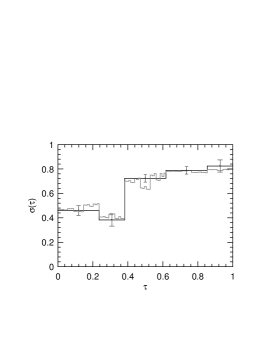
Figure 5: Experimental (in gray) and theoretical (in black) scaling functions. The large steps of the experimental scaling function should be compared at the left part of each step.

I would like to conclude that even though trajectory scaling functions are complicated to define (specially when compared to the $f(\alpha)$ spectrum of scalings) it is possible to extract them from experimental data. To be successful one must be careful that the control parameters are tuned with enough precision for the length of the orbit used.

This work was funded by the Department of Energy.

References

- [1] N. H. Packard, J. P. Crutchfield, J. D. Farmer, and R. S. Shaw. Geometry from a time series. Physical Review Letters, 45:712 – 716, 1980.
- [2] Floris Takens. Detecting strange attractors in turbulence. In Lecture Notes in Mathematics 898, pages 366–381. Springer, Berlin, 1981.
- [3] Mitchell J. Feigenbaum. Some characterizations of strange sets. Journal of Statistical Physics, 46:919–924, 1987.
- [4] Predrag Cvitanović. Invariant measurements of strange sets in terms of cycles. Physical Review Letters, 61:2729–2732, 1988.
- [5] Mitchell J. Feigenbaum. The transition to aperiodic behavior in turbulent systems. Communications of Mathematical Physics, 77:65 – 86, 1980.
- [6] D. Sullivan. Differentiable structures determined by fractal like sets, determined by intrinsic scaling functions on dual Cantor sets. In P. Zweifel, G. Gallavotti, and M. Anile, editors, Non-linear evolution and chaotic phenomena. Plenum, New York, 1987.
- [7] E. B. Vul, Ya. G. Sinai, and K. M. Khanin. Feigenbaum universality and the thermodynamic formalism. Uspekhi Mat. Nauk., 39:3–37, 1984.
- [8] David Ruelle. Thermodynamic Formalism. Addison-Wesley, Reading, 1978.
- [9] R. E. Ecke. Quasiperiodicity, mode-locking, and universal scaling in Rayleigh-Bènard convection. In R. Artuso, P. Cvianović, and G. Casati, editors, Chaos, order, and patterns, volume 280 of NATO ASI series, pages 77–108. Plenum, New York, 1991.
- [10] S. J. Shenker. Scaling behavior of a map of the circle onto itself: emperical results. Physica D, page 405, 1982.
- [11] R. Ecke, Ronnie Mainieri, and T. Sullivan. Universality in quasiperiodic Rayleigh-Bérnard convection. Physical Review A, 44(12):8103–8118, December 1991.
- [12] Mitchell J. Feigenbaum. Presentation functions and scaling function theory for circle maps. Nonlinearity, 1:577–602, 1988.
- [13] C. de Boor. A practical guide to splines. Springer-Verlag, New York, 1978.