On the equality of Hausdorff and box counting dimensions

Abstract

By viewing the covers of a fractal as a statistical mechanical system, the exact capacity of a multifractal is computed. The procedure can be extended to any multifractal described by a scaling function to show why the capacity and Hausdorff dimension are expected to be equal.

1 Introduction

The strange sets that arise in the study of dynamical systems are difficult to characterize and to compare with theoretical predictions. A simple test to check if two strange sets are not smooth distortions of each other is to compare their fractal dimensions: if the fractal dimensions differ, then the sets are not related. There are two widely used definitions of fractal dimensions: the Hausdorff dimension and the capacity (or box counting) dimension. They have long been conjectured [1, 2, 3] to be numerically equal for fractals generated by smooth dynamical systems, even though they are not equal in general [1].

The Hausdorff dimension and the capacity dimension have similar definitions. In both cases we measure how the sum of the boxes in a cover of the fractal scales as the largest box is taken to zero, but in the Hausdorff case the sum is minimized by allowing different box sizes. It is the minimization that gives the Hausdorff dimension its theoretical advantage, as it excludes pathologies that may arise in the limit of smaller boxes and countably many isolated points. Due to the minimization procedure in its definition, the Hausdorff dimension is invariant under diffeomorphisms, while the capacity is invariant under a more restrictive set of transformations: those that transform the metric into an equivalent metric [4].

The Hausdorff dimension has a larger theoretical interest, but it is capacity like dimensions that are usually determined experimentally, as current algorithms make no attempt to optimize the coverings. The now standard procedure of Packard et al. [5] and Takens [2] reconstructs the attractor up to arbitrary coordinate transformations under which the capacity may not be invariant (see examples in [4]).

Here we show that the two dimensions agree for fractals that are described by rapidly convergent scaling functions. The scaling function relates successive refinements of covers of the fractal which can be organized in a tree, the branches indicating how a subcover was refined. The different branches of the tree are then considered as different configurations of a canonical ensemble where the energy of the configuration is proportional to the size of the subcover represented by the branch. Scaling functions and related concepts have received little discussion in the physics literature, so I will present the basic ideas through a simple example. In section 2 we use the scaling function to describe a four scale Cantor set and show how this description is related to a presentation function, or its inverse, a set of contractions that generate the same set. Different ways of organizing the tree correspond to different ways of describing the same set. The capacity is related to the microcanonical ensemble and the corresponding tree is denoted a capacity tree. This notion turns out to be useful in analyzing box counting concepts such as lacunarity, local scaling, and convergence rates, not all explored here. In section 2 we also exactly compute the capacity of a multifractal with equiprobable boxes. The methods of section 2 will be generalized to arbitrary fractals described by scaling functions in section 3 where the equality of the two dimensions is established.

2 Capacity of a multifractal

Most of the fractals that arise in the study of physical systems cannot be described by a simple number, such as the fractal dimension. In a simple deterministic fractal any of its part is an exact rescaling of the whole, but this is not always the case. As observed by Frisch and Parisi [6], different parts of the fractal have to be rescaled by different amounts to resemble the whole, and they are better described by a multitude of scales — they are multifractals. One way of describing a multifractal is in analogy with the middle-third Cantor set: by a sequence of covers that converge to the points of the set. The covers can be described by a subtraction processes, where the middle third of every cover is removed to generate a new set of covers. They can also be described by a contraction processes, where the covers at one level get contracted and translated to generate the new set of covers. The contraction processes is not as well known as the subtraction processes, but it is closer in spirit to the way fractals are generated in dynamical systems.

A simple example of a multiscale fractal on a binary tree is the four-scale Cantor set. We start with two initial segments, the initial conditions $\Delta^{(1)}(0)$ and $\Delta^{(1)}(1)$. The segment $\Delta^{(1)}(0)$ is contracted by $\sigma_{00}$ and $\sigma_{10}$ producing two new segments $\Delta^{(2)}(0,0)$ and $\Delta^{(2)}(1,0)$; and the segment $\Delta^{(1)}(1)$ is contracted by $\sigma_{01}$ and $\sigma_{11}$ producing $\Delta^{(2)}(0,1)$ and $\Delta^{(2)}(1,1)$ as in figure 1. The next level of segments is again obtained by contracting the existing segments by one of the four factors. At each level the parent segment $\Delta^{(n)}(\varepsilon_{n},\ldots,\varepsilon_{1})$ produces two new segments at the ratio

Figure 1: Covers of the four scale Cantor set

$$\frac{|\Delta^{(n+1)}(\varepsilon_{n+1},\ldots,\varepsilon_{1})|}{|\Delta^{(n)}(\varepsilon_{n},\ldots,\varepsilon_{1})|}=\sigma_{\varepsilon_{n+1},\varepsilon_{n}}$$

with the convention that $\varepsilon=0$ is the left contraction and that $\varepsilon=1$ is the right contraction. This construction can be generalized by letting the child segments depend on more than the last two bits, as is the case in the period doubling scenario. We can also allow certain values of the scaling function to be one, as long as every segment goes to zero length as the number of levels goes to infinity. The segments produced by this method are naturally organized in a binary tree, as each parent segment gives rise to two child segments.

Taking the limit of this refinement process produces the fractal. We are not restricted in this description to one (topological) dimension: we could have used squares that get divided into smaller squares instead. In general the scaling function that describes a fractal is not unique, depending on how the segments are labeled.

The distinction between fractals and multifractals comes when we describe them in the way of Hutchinson [7]. This is a characterization of fractals through a dynamics that generates them. A fractal $\cal F$ is a compact set of points of the Euclidean space that is invariant under a finite set of $Q$ contractions $\{\omega_{i}\}$. The set $\cal F$ satisfies

$${\cal F}=\bigcup_{1\leq i\leq Q}\omega_{i}({\cal F})$$

with the condition that the images of different $\omega_{i}$ are contained in opens that do not overlap. The last condition may be relaxed to the intersection of images being a countable set or set of zero Hausdorff measure. The slowest contraction rate of a transformation $\omega_{k}$ is its contraction rate $s_{k}$. If we measure distances in the Euclidean space with $d(\cdot\>,\cdot)$, then for every pair of points $x$ and $y$ of the fractal $\cal F$, the number $s_{k}$ satisfies

$$\begin{array}[]{c}d(\omega_{k}(x),\omega_{k}(y))\leq s_{k}d(x,y)\\ 0<s_{k}<1\end{array}\mbox{ .}$$ (1)

To fix a particular $s_{k}$ we choose the minimum of all numbers that satisfy the inequalities. If the $\omega_{i}$ are uniform contractions, i.e., in (1) we have an equality instead of an inequality, the fractal $\cal F$ is uniformly self-similar. In this case it can be shown that the contractions are the composition of a rotation, a translation and a uniform contraction by the rate $s_{k}$ (see Hutchinson [7]). For uniformly self-similar fractals one has the result:

Theorem (Hutchinson) If $\cal F$ is uniformly self-similar then the capacity and the Hausdorff dimension are numerically equal. In this case the dimension $D$ is the unique root of the equation

$$s_{1}^{D}+s_{2}^{D}+\cdots+s_{Q}^{D}=1\mbox{\ \ .}$$

See [7] for the proof and a partial converse. Many more details on uniformly self-similar fractals can be found in the book by Barnsley [8].

Most fractals that arise from dynamical systems are not uniformly self similar and therefore multifractal, but still it is conjectured [1, 2, 3] that the capacity and the Hausdorff dimension are numerically equal. The Feigenbaum set, the Arnold tongue structure of the sine circle map, and the orbit of the irrational winding number of a critical circle map are all examples of multifractals.

To show that a four scale Cantor set is a multifractal, and therefore Hutchinson’s theorem does not apply, we consider the segments that cover the set, $\Delta^{(n)}(\varepsilon_{n},\ldots,\varepsilon_{1})$, and how they can be transformed into each other. The segments are organized by levels, there being $2^{n}$ segments at level $n$. All the segments at level $n$ in one region of the set can be expressed in terms of the segments of another region one level above, i.e.,

$$|\Delta^{(n)}(\varepsilon_{n},\ldots,\varepsilon_{1})|=|\Delta^{(n-1)}(\varepsilon_{n},\ldots,\varepsilon_{2})|\sigma_{\varepsilon_{2},\varepsilon_{1}}\frac{|\Delta^{(1)}(\varepsilon_{1})|}{|\Delta^{(1)}(\varepsilon_{2})|}\mbox{\ \ .}$$

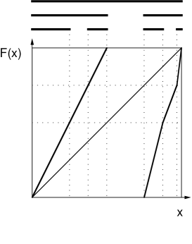
Figure 2: Presentation function for the four scale Cantor set. The first few stages of the construction and how it relates to the slopes is indicated over the plot.

As this relation holds for any $n$, it will hold for a region as small as needed and therefore for all points of the fractal. As $\varepsilon_{1}$ and $\varepsilon_{2}$ can assume two values each, there will be four such relations and we conveniently arrange them into a function $F(\cdot)$ as indicated in figure 2. We have chosen the scalings to be 1/2, 1/4, 1/2 and 1/8 and the two initial segments to be 1/2 and 1/4 of the unit interval. It is actually the inverse of the slopes that are plotted, and the function has been arbitrarily defined to be linear and continuous in the intervals $[1/4,3/8]$ and $[7/8,31/32]$. The four scale Cantor set will then be the set of points that remain in the interval under forward iterations of $F$. The function $F$ is a presentation function for the four scale Cantor set, and its inverse has two branches:

$$\begin{array}[]{lr}\omega_{1}(x)=F^{-1}(x)&x\in\Delta^{1}(0)\\ \omega_{2}(x)=F^{-1}(x)&x\in\Delta^{1}(1)\end{array}\mbox{\ \ ,}$$

the contractions to be used in Hutchinson’s characterization of fractals. As $\omega_{1}$ and $\omega_{2}$ are non-uniform contractions, the fractal is not uniformly self-similar. The presentation function is not unique, but one can show, by considering all other ways of organizing the slopes, that any other presentation function yields a set of non-uniform contractions. From figure 2 one can see how to construct a presentation function given the first steps generated by the scaling function. This procedure allows us to go from the scaling function description to the presentation function description as required. The alternative description of multifractals by scaling functions was introduced by Feigenbaum [9]. He later on showed that fractals could also be described with presentation functions [10, 11].

Given the scaling function, or the presentation function, or the the set of contractions $\omega_{i}$, one can compute the Hausdorff and capacity dimensions of the generated fractal. To determine the Hausdorff dimension we first consider the $\beta$-Hausdorff measure $Z(\beta)$ of the set, computed from its coverings $\Delta$ and defined as

$$Z(\beta)=\lim_{l\rightarrow 0}\inf_{|\Delta|<l}\sum_{\varepsilon}|\Delta(\varepsilon)|^{\beta}$$

The infimum is over all countable covers with segments smaller than $l$ and the sum is over the segments of the cover. The measure of the set is zero or infinity for almost all values of $\beta$, and there is a unique $\beta$, the Hausdorff dimension $\beta_{H}$, that separates these two domains of $Z$. Numerically the infimun is difficult to determine, and it is convenient to consider the covers from a grid of boxes of side $l$, so there is no need to optimize the covers by taking the infimum. The capacity dimension will be the number that separates the zero and the infinity domain of $Z$, just like in the Hausdorff case. In the capacity case all terms of the sum are the same and if $N(l)$ boxes are needed to cover the set, the capacity dimension $\beta_{C}$ is written as

$$\beta_{C}=-\lim_{l\rightarrow 0}\frac{\ln N(l)}{\ln l}\mbox{\ \ ,}$$ (2)

when the limit exists.

If the segments of the covers were all generated from a (translational invariant) scaling function we can identify $Z$ with the partition function of a thermodynamical system with energy $-\ln|\Delta(\varepsilon)|$. For the four scale Cantor set we can write

$$|\Delta^{(n)}(\varepsilon_{n},\ldots,\varepsilon_{1})|=\sigma_{\varepsilon_{n},\varepsilon_{n-1}}\ldots\sigma_{\varepsilon_{3},\varepsilon_{2}}\sigma_{\varepsilon_{2},\varepsilon_{1}}|\Delta^{(1)}(\varepsilon_{1})|\stackrel{{\scriptstyle\rm def}}{{=}}\exp(-u(\varepsilon_{n},\ldots,\varepsilon_{1}))$$

and

$$Z^{(n)}(\beta)=\sum_{\varepsilon}\exp(-\beta u^{(n)}(\varepsilon))$$

To complete the identification we must take the limit $n\rightarrow\infty$. From the partition function we can compute the pressure at inverse temperature $\beta$ in the thermodynamic limit from

$$-p(\beta)=\lim_{n\rightarrow\infty}\frac{1}{n}\log(\sum|\Delta^{(n)}(\varepsilon)|^{\beta})\mbox{\ \ .}$$ (3)

The name pressure is used rather than free energy per particle per temperature degree because the limit of the logarithm of the partition function can be identified with the pressure in the case of a lattice gas in the grand-canonical ensemble. Vul, Sinai and Khanin [12] and Ruelle [13] have shown that the Hausdorff dimension $\beta_{H}$ is the unique number for which the pressure satisfies the Bowen-Ruelle formula

$$p(\beta_{H})=0\mbox{\ \ .}$$

Using transfer matrix techniques to evaluate the partition function, Feigenbaum [14] has shown that the Hausdorff dimension of the four scale Cantor set is the root of

$$\frac{\sigma^{\beta}_{00}+\sigma^{\beta}_{11}+\sqrt{(\sigma^{\beta}_{00}+\sigma^{\beta}_{11})^{2}-4\sigma^{\beta}_{01}\sigma^{\beta}_{10}}}{2}=1\mbox{\ \ .}$$

For the scaling coefficients we are considering the root is $\beta_{H}=0.640602307$.

We can also determine the capacity of the fractal from the partial coverings given by the segments. To determine the capacity of the set we must count how many boxes (segments) of a given size are needed to cover the set. At level one we would need two boxes of size 1/2 to cover the set, while if we had used a box size of 1/8, apparently six boxes would be necessary at level one. This is an overestimate, as further refinement of the cover shows that only five boxes are required. One should be careful not to confuse the covers of the Cantor set with the set itself. The boxes of the grid must cover the set and not one of its covers. To count how many boxes of a given size cover the set, each sub-cover should be refined until it is smaller than the current box size, and the final number of boxes counted.

Figure 3: Labeling scheme for the capacity tree. The branch labels are explained in section 2 and the segment labels in section 3.

This suggest another organization of the fractal. Instead of contracting every segment by one of the values of the scaling function, we fix a box contraction rate per level and at each level contract the covers that are larger than the current box size. As the box size goes to zero with increasing levels of the construction, the final set will the same. As the slowest contraction rate is 1/2 we will reduce the box size by a factor of two at each level. This means that the segment that gets scaled by the factor of 1/8 only needs to be contracted at every three levels, while the segment that gets scaled by 1/4, at every two levels, and the segment that gets scaled by 1/2, at every level. We now introduce another symbolic labeling for the segments: each segment gets a 0, 1, or 2 according to how many levels it can go without contracting. As we started with a box size of one and took a 1/2, 1/4 contraction to generate the two initial segments, they can also be labeled according to the new scheme. In figure 3 we have the the first few levels of coverings, with the labels for counting indicated on the arrows and two segments labeled as described in section 3.

At each level, if a segment has a label 0 it produces two daughters, and if it has a label bigger than zero it copies itself at the next level, but with a label one unit smaller. If we read the branches of the tree as words built from the alphabet 0, 1, 2 the rules for the construction of all the branches at one level are:

$$\begin{array}[]{rcl}x2&\mapsto&x21\\ x1&\mapsto&x10\\ x10&\mapsto&x100,x102\\ x00&\mapsto&x000,x001\end{array}$$

where $x$ stands for any partial word. One can see by inspection that these are the rules used for constructing the tree in figure 3. With the use of these rules we can write relations between the number of leaves (or words) of one kind with the number of leaves at previous levels. If $N_{0}(n)$ denotes the number of segments that have the label 0 at level $n$, and $N_{1}(n)$ and $N_{2}(n)$ the number of segments with the other labels, we have that

$$\begin{array}[]{rcl}N_{0}(n)&=&N_{0}(n-1)+N_{1}(n-1)\\ N_{1}(n)&=&N_{0}(n-1)-N_{1}(n-2)+N_{2}(n-1)\\ N_{2}(n)&=&N_{1}(n-2)\end{array}$$

with the initial conditions

$$\begin{array}[]{c}N_{1}(0)=N_{2}(0)=N_{2}(1)=0\\ N_{0}(0)=N_{0}(1)=N_{1}(1)=1\end{array}\mbox{\ \ .}$$

To solve the system of recurrences we use the generating function method. We will solve for $N_{0}$ as zeros dominate the tree. Let $\Gamma_{0}(x)$ be the generating function for the the number of segments with label 0 at level $n$,

$$\Gamma_{0}(x)=\sum_{n\geq 0}N_{0}(n)x^{n}\mbox{\ \ .}$$

By solving the system of recurrences for $N_{0}$ we get

$$N_{0}(n)-2N_{0}(n+1)-N_{0}(n+3)+N_{0}(n+4)=0\mbox{\ \ .}$$

In multiplying by $x^{n}$, summing for $n\geq 0$ , and subtracting a few initial terms, we get that

$$\Gamma_{0}(x)=-\frac{x^{3}-x^{2}-1}{x^{4}-2x^{3}-x+1}\mbox{\ \ .}$$ (4)

The same procedure can be used for obtaining the generating functions for the number of segments with label 1, $\Gamma_{1}$, and with label 2, $\Gamma_{2}$. The generating function for the total number of boxes at each level is given by the sum of all three generating functions:

$$\Gamma(x)=\Gamma_{0}(x)+\Gamma_{1}(x)+\Gamma_{2}(x)=\frac{x^{2}+x+1}{x^{4}-2x^{3}-x+1}=\sum_{n\geq 0}N(n)x^{n}\mbox{\ \ .}$$

The generating function can be expanded in a Taylor series around zero and the term in $x^{n}$ picked out to give $N(n)$. This can be done by factoring the generating function in partial fractions. Each linear term is then expanded according to the relation

$$\frac{1}{1-ax}=\sum_{n\geq 0}(ax)^{n}$$

and we see that the leading behavior of the term in $x^{n}$ is of the form

$$N(n)\rightarrow(\mbox{const})(1/r_{1})^{n}$$

as $n\rightarrow\infty$ and where $r_{1}$ is the smallest root of the denominator in absolute (4) value. The roots of the polynomial are given in table 1.

root	value
$r_{1}$	$0.641\,445$
$r_{2}$,$r_{3}$	$0.858\,004e^{\pm i0.458\,255}$
$r_{4}$	$2.177\,689$

Table 1: Poles of the generating function

The exact capacity of the four-scale Cantor set can be determined from the asymptotic behavior. We get that

$$\beta_{C}=-\frac{\ln r_{1}}{\ln 2}=0.640602307\mbox{\ \ .}$$

in complete agreement with the Hausdorff dimension determined by the thermodynamical formalism. We can verify that $\beta_{C}$ and $\beta_{H}$ are the same number by verifying that they satisfy the same algebraic equation.

The above expression for the number of boxes, $N(n)$, needed to cover the Cantor set is an exact expression for a multiscale Cantor set and it is qualitatively different from the expression for the number of boxes for a uniform scale Cantor set.

3 The equality of Hausdorff and capacity dimensions

We now want to show that the capacity and the Hausdorff dimensions are the same for a multiscale Cantor set. We will only consider multiscale Cantor sets that are described by a Feigenbaum scaling function on a binary tree (like the period doubling tree). These Cantor sets not only have the compact description offered by scaling function, but they also have a finite Hausdorff measure (see Hutchinson [7]). We can easily generalize to trees that have a bounded number of branches per node.

When the scaling function is of infinite range an infinite amount of initial segments are needed to produce the first level of refinement. To avoid having to specify an infinite amount of segments we choose an approximation scheme to generate initial segments. It will turn out that the thermodynamic quantities of the set are independent of this scheme. At level $n$ we want to compute

$$Z^{(n)}(\beta)=\sum_{\varepsilon}|\Delta^{(n)}(\varepsilon)|^{\beta}$$

with $\varepsilon$ running over all possible configurations. We approximate

$$|\Delta^{(n)}(\varepsilon_{n},\ldots,\varepsilon_{1})|=$$

$$\sigma(\varepsilon_{n},\ldots,\varepsilon_{1},0,0,\ldots)\sigma(\varepsilon_{n-1},\ldots,\varepsilon_{1},0,\ldots)\ldots\sigma(\varepsilon_{1},0,\ldots)|\Delta_{0}|$$

by padding the scaling function with zeros. For the uniqueness of the thermodynamic quantities the variation of the scaling function decreases for bits to the right,

$$|\sigma(\ldots,\varepsilon_{n}=1,\ldots)-\sigma(\ldots,\varepsilon_{n}=0,\ldots)|<f(n)$$ (5)

where $f(n)$ goes to zero faster than $1/n^{2}$ as $n$ goes to infinity. This is equivalent to the uniqueness of the Gibbs state (see Simon’s lemma [15]). A consequence of the uniqueness is that the thermodynamic properties are independent of the boundary condition, and for the purpose of computing these properties almost any choice of boundary will do, and that is why we need not specify an infinite number of initial conditions.

To compute the capacity we must evaluate its defining limit (2). The function $N(l)$ is piecewise constant, as it takes values over the integers, and monotonically increasing, as a refinement cannot decrease the number of boxes required to cover the set. If the capacity of the set is well defined, then we can choose any sequence $l_{n}$ of box sizes as long as $l_{n}\rightarrow 0$ as $n\rightarrow\infty$, and evaluate the limit of the sequence of ratios

$$\beta_{C}=-\lim_{l\rightarrow 0}\frac{\ln N(l)}{\ln l}=-\lim_{n\rightarrow\infty}\frac{\ln N(l_{n})}{\ln l_{n}}\mbox{\ \ .}$$

The covers $\Delta^{(n)}(\varepsilon)$ can be converted into a new sequence of covers as long as we still have the convergence to zero box size. We fix the contraction rate $b$ of the grid of boxes to be the slowest contraction rate of any child segment, that is,

$$b=\sup_{\varepsilon}\;\sigma(\varepsilon)<1\mbox{\ \ .}$$

If we denote the new covers by $\Delta^{(n)}_{C}(\varepsilon)$ then they will satisfy

$$cb^{n}|\Delta_{0}|\leq|\Delta^{n}_{C}(\varepsilon)|\leq b^{n}|\Delta_{0}|$$ (6)

where $c$ is the non-zero infimum of the scaling function over all configurations $\varepsilon$. This can be seen as tree where the segments contract only if at the next level they were to be larger than the box size at that level. This tree — the capacity tree — allows us to define a new scaling function.

The capacity tree is a different set of covers that converge to the same set. Each point $x$ of the fractal can be uniquely defined by the set of segments that contain it,

$$\Delta_{0}\supset\Delta_{C}^{(1)}(\varepsilon_{1})\supset\Delta_{C}^{(2)}(\varepsilon_{2},\varepsilon_{1})\supset\ldots\ni x$$

and the sequence of $\varepsilon_{i}$ are the unique configuration associated with the point $x$ and they are used to label the covers as done in figure 3. This uniqueness establishes a one-to-one correspondence between the limit points of the capacity tree and the Hausdorff tree. It is important to realize that the points of the Cantor set do not change when we go from the Hausdorff tree to the capacity tree, only the sequence of covers that approach them. The sequence of covers approaching a point in the Hausdorff tree and the capacity tree do not differ, only their labels do.

We can now use the new sequence of covers $\Delta^{(n)}_{C}(\varepsilon)$ in formula (3) to compute the Hausdorff dimension. As the set is the same, the Hausdorff dimension will not change. This will be the case if the original scaling function fell off exponentially, for the transformation to the capacity tree just changes the rate of fall off of $f(n)$ in (5). But if the original scaling function were bounded by power law fall off, $f(n)=n^{-p}$, then there will be cases when the re-arrangement cannot be done even with a unique Gibbs state.

To compute the capacity we rewrite the limit (2) in terms of thermodynamical quantities. $N(n)$ is the number of segments at the level $n$, and by the construction of the capacity tree

$$N(n)=\mbox{card}\{\Delta^{(n)}(\varepsilon):cb^{n}|\Delta_{0}|\leq|\Delta^{(n)}_{C}(\varepsilon)|\leq b^{n}|\Delta_{0}\}\mbox{\ \ .}$$

The bounds for $|\Delta^{(n)}_{C}(\varepsilon)|$, equation (6), tell us that $(\ln|\Delta^{(n)}_{C}|)/n$ is approaching a limit as $n\rightarrow\infty$. It differs from this limit by at most $-(\ln c|\Delta_{0}|)/n$, a small quantity we shall call $\delta_{n}$. The number of occupied boxes at level $n$ can be written as

$$N(n)=\mbox{card}\{\Delta^{(n)}(\varepsilon):|\frac{1}{n}\ln|\Delta^{(n)_{C}}(\varepsilon)|-\ln b|\leq\delta_{n}\}\mbox{\ \ .}$$

By comparing the expression for $N(n)$ with the definition of entropy in the microcanonical (see the lectures by Lanford [16]), we see that in the limit $n$ goes to infinity $(\ln N(n))/n$ is the entropy of the states with energy $\ln b^{-1}$. Also $l_{n}$ can be expressed in terms of $\ln b$. Combining these results the capacity can be expressed as the ratio of the entropy to the energy in the microcanonical ensemble,

$$\beta_{C}=\frac{\displaystyle\lim_{n\rightarrow\infty}\frac{1}{n}\ln N(n)}{\displaystyle\lim_{n\rightarrow\infty}\frac{1}{n}\ln l_{n}}=\frac{s(u)}{u}\mbox{\ \ .}$$ (7)

The capacity tree corresponds to a statistical mechanical system where all the states have the same energy $u$. If the energy can only assume one value, then the entropy is also only defined at that single point. To relate this to the canonical description we have to Legendre transform the energy to get the free energy, or alternatively, transform the entropy to get the pressure. In this case we cannot compute the derivative of the entropy to get the inverse temperature $\beta$ of the system because the entropy is only defined at a point. But the thermodynamical formalism is more general, and the Legendre transform can be performed just with continuity.

If $f(x)$ is a convex function its Legendre transform is given by the following procedure: pick any real number $p$ and consider the real line $y=xp$; the maximum signed distance (not including infinity) between the curve $f(x)$ and the line $y=xp$ along the vertical is the Legendre transform of $f$ for the value $p$. This reduces to the usual definition when $f$ is differentiable.

The Legendre transform of the entropy is then a line. If $s_{0}$ is the unique value of the entropy and $u_{0}$ the unique value of the energy, the pressure as a function of Legendre variable $\beta$ is

$$p(\beta)=\beta u_{0}-s_{0}\mbox{\ \ .}$$

For the Hausdorff dimension, $\beta_{H}$, we have that $p(\beta_{H})=0$ and, as both computations are for the same set of states,

$$\beta_{H}=\frac{s_{0}}{u_{0}}=\beta_{C}$$

according to equation (7), establishing the equality of the two dimensions.

4 Conclusion

With the aid of the thermodynamic formalism we have shown (within the precision of a physicist) that for a fractal described by a scaling function that falls off exponentially, the capacity and the Hausdorff dimension will be numerically equal. If the fractal is generated from the iterations of a differentiable presentation function, then the scaling function will fall off exponentially fast, the rate related to its Holder exponent. The equality may hold in less restrictive conditions, as we only need the existence and uniqueness of the ratio (7) between the entropy and the energy. Even when there is more than one Gibbs state the ratio may be the same in each state due to a symmetry of the scaling function. The ease in which the result was established is due to the use of the scaling functions. They play the role of the interaction in the thermodynamics of iterated functions. If instead we had started with the derivative of the iterating map, the analysis would become more difficult.

Not every map leads to an exponentially decaying scaling function. The most common exception is for maps that display intermittency. In this case the scaling function will have a power law decay — in equation (5), $f(n)=n^{-s}$. In most cases $s<2$ indicating that the generalized dimensions of the set have a phase transition. For this case the Hausdorff tree and the capacity tree are not equivalent, as they cannot be re-arranged into each other.

Obtaining the scaling function from the map, and proving it unique, has only been done in a few cases. One can intuitively see the difficulties by noticing that when we constructed the presentation function for the four scale Cantor set, we had the freedom to define the map arbitrarily in the pre-image of the gap, i.e., for $F^{-1}([1/2,3/4])$. For any choice in the gap pre-image we would had obtained the same scaling function and the same limit set. This arbitrariness extends to all pre-images of the gap, that is, the presentation function is arbitrary for most points. It is the product of the slopes of the presentation function at the points of the limit set that determine the scaling function, a property that seems difficult to control with a priori bounds. If however we start our analysis from the scaling function or the presentation function we can easily determine the thermodynamic quantities from them.

References

- [1] J. D. Farmer, Edward Ott, and James A. Yorke. The dimension of chaotic attractors. Physica D, 7:153–180, 1983.
- [2] Floris Takens. Detecting strange attractors in turbulence. In Lecture notes in Mathematics 898, pages 366–381, Berlin, 1981. Springer.
- [3] Thomas C. Halsey et al. Fractal measures and their singularities: the characterization of strange sets. Physical Review A, 33:1141–1151, 1986.
- [4] E. Ott, W. D. Withers, and J. A. Yorke. Is the dimension of chaotic attractors invariante under coordinate changes? Journal of Statistical Physics, 36:687 – 697, 1984.
- [5] N. H. Packard et al. Geometry from a time series. Physical Review Letters, 45:712 – 716, 1980.
- [6] U. Frisch and G. Parisi. On the singularity structure of fully developed turbulence. In M. Ghil, R. Benzi, and G. Parisi, editors, Varanna School LXXXVIII, International School of Physics “Enrico Fermi”, pages 84–88. North-Holland, Amsterdam, 1985.
- [7] J. Hutchinson. Fractals and self similarity. Indiana Univ. Math. J., 30:713 – 747, 1981.
- [8] Michael Barnsley. Fractals Everywhere. Academic Press, San Diego, 1988.
- [9] Mitchell J. Feigenbaum. The transition to aperiodic behavior in turbulent systems. Communications of Mathematical Physics, 77:65 – 86, 1980.
- [10] Mitchell J. Feigenbaum. Presentation functions, fixed points, and a theory of scaling function dynamics. Journal of Statistical Physics, 52:527–569, 1988.
- [11] Mitchell J. Feigenbaum. Presentation functions and scaling function theory for circle maps. Nonlinearity, 1:577–602, 1988.
- [12] E. B. Vul, Ya. G. Sinai, and K. M. Khanin. Feigenbaum universality and the thermodynamic formalism. Uspekhi Mat. Nauk., 39:3–37, 1984.
- [13] D. Ruelle. Bowen’s formula for the hausdorff dimension of self-similar sets. In Jürg Fröhlich, editor, Scaling ans self-similarity in physics, volume 7 of Progress in Physics, pages 351–358. Birkhaäser, Boston, 1983.
- [14] Mitchell J. Feigenbaum. Some characterizations of strange sets. Journal of Statistical Physics, 46:919–924, 1987.
- [15] Barry Simon. Comm. Math. Phys., 68:183, 1979.
- [16] Oscar E. Lanford III. Entropy and equilibrium states in classical statistical mechanics. In Lecture Notes in Physics, volume 28. Springer, Berlin, 1973.