Hypersensitivity to Perturbations in the Quantum Baker’s Map

Abstract

We analyze a randomly perturbed quantum version of the baker’s transformation, a prototype of an area-conserving chaotic map. By numerically simulating the perturbed evolution, we estimate the information needed to follow a perturbed Hilbert-space vector in time. We find that the Landauer erasure cost associated with this information grows very rapidly and becomes much larger than the maximum statistical entropy given by the logarithm of the dimension of Hilbert space. The quantum baker’s map thus displays a hypersensitivity to perturbations that is analogous to behavior found earlier in the classical case. This hypersensitivity characterizes “quantum chaos” in a way that is directly relevant to statistical physics.

Great progress has been made in studying manifestations of chaos in quantum systems [1], yet there still is controversy as to whether quantum chaos exists at all [2, 3]. A chief reason for this is that the most important characteristic of classical chaotic systems—exponential divergence of trajectories starting at arbitrarily close initial points in phase space—is absent from quantum systems simply because the existence of a quantum scale makes meaningless the concept of two arbitrarily close points in phase space.

Any attempt to find exponential divergence of trajectories of Hilbert-space vectors founders immediately, because the linear Schrödinger equation, with its unitary evolution, preserves Hilbert-space inner products. Yet the unitary linear evolution of the Schrödinger equation must be irrelevant to the issue of quantum chaos [2], since any Hamiltonian classical chaotic system can be described by an analogous area-conserving linear Liouville equation. Two probability distributions in classical phase space—we call these phase-space patterns—that are initially close together (in terms of an overlap integral) stay close together forever, because the Liouville equation is area conserving. This leads to the question we address in the present article: Are there manifestations of Hamiltonian classical chaos in the Liouville equation that are also present in quantum mechanics?

In an earlier paper [4] we analyzed a prototype of an area-conserving chaotic map, the baker’s transformation [5], in the Liouville representation; i. e., we focused on phase-space patterns instead of on single trajectories. Our analysis was guided by the question [6] of how available work decreases with time when the baker’s map is subjected to area-conserving random perturbations. An area-conserving abstract mapping corresponds to an energy-conserving phase-space system, so we identify two negative contributions to free energy. The conventional one is ordinary entropy, which measures how incomplete knowledge about a system reduces our ability to extract work. The other contribution arises from Landauer’s principle [7, 8] that there is an unavoidable energy cost of $k_{B}T\ln 2$ connected with the erasure of one bit of information. It follows from Landauer’s principle that the information, quantified by algorithmic information [9], needed to give a complete description of a system state also reduces the amount of available work and thus should make a further negative contribution to free energy [10, 11].

In our earlier paper [4] we compared two strategies for preserving the ability to extract work from a system. The first strategy is to keep track of the perturbed phase-space pattern in fine-grained detail, in an attempt to preserve the work inherent in the initial condition. The second strategy, which we call coarse graining, is to average over the perturbation and to put up with the resulting ordinary entropy increase. We found, for the perturbed baker’s map, that the information needed to implement the first strategy is overwhelmingly larger than the entropy increase of the second strategy. This means that the free-energy cost of tracking the perturbed pattern in fine-grained detail is enormous and far greater than the cost of the entropy increase that results from coarse graining. We conjecture that this hypersensitivity to perturbations is a general feature of perturbed classical chaotic systems, and we regard it as the desired manifestation of classical chaos in the Liouville equation.

In the present paper we compare the two strategies for preserving work in the case of a quantum system, a quantum version of the baker’s map [12]. Using numerical simulation, we find essentially the same behavior as in the classical case, as was suggested using heuristic arguments in Ref. [6]. The quantum baker’s map displays hypersensitivity to perturbations and thus can be said to exhibit quantum chaos.

The concept of algorithmic information has been used before to investigate quantum chaos [2, 13]. If one defines a chaotic system as one where the algorithmic information needed to predict a single (unperturbed) trajectory grows linearly with time (or number of steps) [14], then there is classical chaos, but no quantum chaos [2]. Our approach, by focusing on patterns in phase space instead of trajectories, uses a framework where classical and quantum mechanics can be treated on analogous footings. Moreover, since Landauer’s principle gives information an explicit physical meaning by connecting it to available work, our characterization in terms of hypersensitivity to perturbations is directly relevant to statistical physics.

The classical baker’s transformation maps the unit square $0\leq q,p\leq 1$ onto itself according to

$$f:(q,p)\longmapsto(2q-[2q],(p+[2q])/2)\;,$$ (1)

where the square brackets denote the integer part. There is no unique way to quantize a classical map. Here we adopt a quantized baker’s map introduced by Balazs and Voros [12] and put in more symmetrical form by Saraceno [15]. Position and momentum space are discretized, placing the lattice sites at half-integer values $q_{j}=p_{j}=(j+1/2)/2N$ for $j=0,\ldots,2N-1$. The dimension $2N$ of Hilbert space is assumed to be even. For consistency of units, let the quantum scale on phase space be $2\pi\hbar=1/2N$. Position and momentum basis kets are denoted by $|q_{j}\rangle$ and $|p_{j}\rangle$. A transformation between these two bases is performed by the operator $G_{2N}$, defined by the matrix elements

$$(G_{2N})_{jk}=\langle p_{j}|q_{k}\rangle=\sqrt{2\pi\hbar}\;e^{-ip_{j}q_{k}/\hbar}\;.$$ (2)

The quantum baker’s map is now defined by the matrix

$$B=G_{2N}^{-1}\left(\begin{array}[]{cc}G_{N}&0\\ 0&G_{N}\end{array}\right)\;,$$ (3)

where, as throughout this article, matrix elements and vector coordinates are given relative to the position basis.

The perturbation operator we use is constructed to resemble the type of perturbation used in our previous work [4] on the classical baker’s map. We partition phase space into an even number $2N_{c}=2N/w_{c}$ of congruent perturbation cells, where $2N_{c}$ and $w_{c}\geq 2$ are integral divisors of $2N$. In the following we use perturbation cells that are vertical stripes extending over the entire $p$ range. Then each perturbation cell contains $w_{c}$ $q$-eigenstates. A perturbation operator that perturbs each perturbation cell independently has the form of a matrix with zero elements everywhere except for $2N_{c}$ square blocks of size $w_{c}$ on the diagonal. We choose these square blocks so that they correspond to a shift in the $p$ direction in a $w_{c}$-dimensional subspace. Let the momentum shift in the $n$th perturbation cell ($n=0,\ldots,2N_{c}-1$) be $\alpha i_{n}$, where the real number $\alpha$ is the magnitude of the momentum shift and $i_{n}\in\{-1,1\}$. The symmetry condition $i_{2N_{c}-n-1}=i_{n}$ ($n=0,\ldots,N_{c}-1$) avoids rapid oscillations and thus ensures similarity to the classical case. The perturbation operator $U_{\alpha;i_{0},\ldots,i_{N_{c}-1}}$ is defined by

$$(U_{\alpha;i_{0},\ldots,i_{N_{c}-1}})_{jk}=\delta_{jk}e^{i2\pi\phi_{k}}\;,$$ (4)

where $\phi_{0}=0$, $\phi_{k}=\phi_{k-1}+\alpha i_{n(k)}$ ($k=1,\ldots,2N-1$) with $n(k)=[k/w_{c}]$. The parameter $\alpha$ characterizes the “strength” of the perturbation, whereas $w_{c}/2N=1/2N_{c}$ is the area of the perturbation cells.

A perturbed time step consists of first applying the unperturbed time-evolution operator $B$, followed by a perturbation operator $U_{\alpha;i_{0},\ldots,i_{N_{c}-1}}$ with $i_{0},\ldots,i_{N_{c}-1}\in\{-1,1\}$ chosen at random, $\alpha$ being fixed. We thus allow for a different perturbation at each step, in contrast to Ref. [16] where a particular perturbed evolution operator was applied repeatedly. After $n$ time steps, the number of different perturbation sequences—or histories—is $2^{nN_{c}}$.

Our specialization to vertically striped perturbation cells involves no restriction relative to our work on the classical baker’s map. There we allowed for $(2^{m}w_{c}/2N)\times 2^{-m}$ rectangular perturbation cells, which are the image of vertical stripes under $m$ applications of the baker’s map, $2^{m}\leq 2N/w_{c}=2N_{c}$. Likewise, the perturbation operator for “rectangular” quantum-mechanical perturbation cells is $U^{\prime}=B^{m}UB^{-m}$ where $U$ is given by Eq. (4). Using $U$ with initial state $|\psi_{0}\rangle$ is equivalent to using $U^{\prime}$ with initial state $B^{m}|\psi_{0}\rangle$. The freedom to choose $m$—we use $m=0$ for vertical stripes—is the same as the classical freedom to choose the initial position of the “decimal point” in the symbolic representation of the baker’s map.

As a preliminary step, we show that perturbed evolution leads after several steps to an ensemble of vectors that is similar to an ensemble of vectors distributed randomly on Hilbert space. A useful criterion for determining the randomness of an ensemble of vectors $|\psi\rangle$ is based on the moments of the quantity [17]

$$W(|\psi\rangle)=-\sum_{i=0}^{2N-1}|\langle q_{i}|\psi\rangle|^{2}\log(|\langle q_{i}|\psi\rangle|^{2})\;,$$ (5)

which we call $W$-entropy to distinguish it from ordinary entropy ($\log$ denotes the binary logarithm, as throughout this paper). For random vectors in $2N=16$-dimensional Hilbert space, the mean and standard deviation of the $W$-entropy are given by $W=3.434\pm 0.178$ bits, a result obtained on a computer by calculating $W(|\psi\rangle)$ for a large number of vectors $|\psi\rangle$ chosen at random from an ensemble distributed uniformly over Hilbert space [17]. (This mean value agrees with the exact formula for the mean value [18], $W=[\Psi(2N+1)-\Psi(2)]/\ln 2$, where $\Psi$ is the digamma function.) We compare the result for random vectors with the first two moments of the $W$-entropy for an ensemble of vectors created by the perturbed baker’s map in a 16-dimensional Hilbert space. Choosing $2N_{c}=2$ and $\alpha=0.025=0.4/2N$, we create an ensemble of approximately 20 000 perturbed vectors by applying different randomly chosen histories for $n=15$ perturbed time steps to the initial vector $|\psi_{0}\rangle=|p_{5}\rangle$. We find for the first two moments of the $W$-entropy the values $W=3.428\pm 0.184$ bits, very close to the moments for a random sample.

As a second check of randomness, we calculate the distribution of Hilbert-space angles $\theta=\cos^{-1}(|\langle\psi^{\prime}|\psi\rangle|)$ between vectors $|\psi\rangle$ and $|\psi^{\prime}\rangle$ that have evolved under the same perturbed quantum baker’s map applied to the same initial state as in the previous example. We compute the Hilbert-space angle between each pair of vectors in each of three ensembles of approximately 16 000 vectors created by applying different randomly chosen perturbation histories for 15, 23, and 31 steps. In addition, we compute the Hilbert-space angle between each pair of the $2^{10}$ vectors after 10 steps. The resulting distributions of Hilbert-space angles are displayed in Fig. 1.

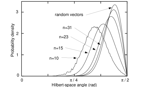
Figure 1: Distribution of Hilbert-space angles for vectors evolving under the perturbed quantum baker’s map, shown for different numbers of perturbed time steps $n$. For comparison, the distribution for random vectors is also shown. The dimension of Hilbert space is $2N=16$, the number of perturbation cells is $2N_{c}=2$, the perturbation strength is $\alpha=0.025=0.4/2N$, and the initial vector is $|\psi_{0}\rangle=|p_{5}\rangle$.

After 31 steps the closest pair of vectors is $27.1^{\circ}$ apart, a striking demonstration of the “size” of 16-dimensional Hilbert space, i. e., of how many widely separated vectors Hilbert space can accommodate even for a relatively small dimension. For comparison, Fig. 1 also shows the distribution $f(\theta)=30(\sin\theta)^{29}\cos\theta$ of Hilbert-space angles for a set of random vectors. These results show clearly how the ensemble is randomized by the perturbed quantum baker’s map.

We proceed now to compare the two strategies for extracting work outlined above—coarse graining versus following the evolved vector in fine-grained detail. We estimate the conditional algorithmic information $\Delta I$ needed—given background information—to specify a typical perturbed vector after $n$ steps and compare it to the increase in ordinary entropy $\Delta H$ that results from averaging over the perturbation. Our first example uses, as before, a $2N=16$-dimensional Hilbert space, partitioned into $2N_{c}=2$ vertically striped perturbation cells. We choose a fixed perturbation amplitude $\alpha=0.025=0.4/2N$ and an initial pure state $|\psi_{0}\rangle=|p_{5}\rangle$, i. e., a momentum eigenstate, which corresponds to a horizontal stripe in the unit square. This perturbation can be described completely by giving one bit per step, to specify which of the two possible perturbation operators $U_{\alpha;1}$ and $U_{\alpha;-1}$ is applied. If the logarithmic term [11] that keeps track of the number of steps $n$ is neglected, this sets an upper bound on the information $\Delta I$. This upper bound is realized only if two different histories of perturbed time steps always lead to two different vectors at some level of resolution on Hilbert space. We choose a resolution that regards two vectors as different if their Hilbert-space angle exceeds $\delta\theta=\pi/50=3.6^{\circ}$ ($|\langle\psi^{\prime}|\psi\rangle|$ smaller than $0.998$). By comparing numerically all possible histories, we find that, through 15 perturbed time steps, all trajectories lead to distinguishable vectors. Figure 2 shows the resulting linear increase in the information $\Delta I$.

Figure 2: Conditional algorithmic information $\Delta I$ needed to track a vector evolving under the perturbed quantum baker’s map, compared to the increase in ordinary entropy $\Delta H$ that results from averaging over the perturbation. The parameters are the same as in Fig. 1.

Figure 3: $\Delta I$ and $\Delta H$ as in Fig. 2, but with parameters $2N=64$, $2N_{c}=16$, $\alpha=0.05\simeq 3/2N$, and $|\psi_{0}\rangle=B^{-5}|p_{1}\rangle$.

Figure 2 also shows the ordinary entropy increase $\Delta H$, obtained by determining the entropy of the density matrix that results from averaging over all possible histories. It can be seen that $\Delta I$ is always larger than $\Delta H$. Indeed, $\Delta H$ saturates at the value $\Delta H_{\rm max}=\log 2N=4$ bits, the logarithm of the dimension of Hilbert space, whereas $\Delta I$ is only limited by $\Delta I_{\rm max}\simeq-2(2N-1)\log(\delta\theta/2)\simeq 150$ bits, which is the logarithm of the number of different vectors Hilbert space can accommodate [6, 19]. Whereas $\Delta H_{\rm max}$ grows logarithmically with the dimension $2N$ of Hilbert space, the maximum information $\Delta I_{\rm max}$ grows linearly with $2N$ and is enormous for macroscopic systems.

As in the classical case [4], the information $\Delta I$ grows more dramatically when the number of perturbation cells is large. Figure 3 displays results for a 64-dimensional Hilbert space with 16 vertically striped perturbation cells, each containing four position eigenstates. The perturbation strength is $\alpha=0.05\simeq 3/2N$, and the initial state is $|\psi_{0}\rangle=B^{-5}|p_{1}\rangle$, a state whose image under $B$ has negligible support outside the leftmost perturbation cell. This means that, in order to describe the perturbed state after the first time step, in the perturbation operator $U_{\alpha;i_{0},\ldots,i_{7}}$ only the sign $i_{0}$ referring to the leftmost perturbation cell must be specified. Since $B^{2}|\psi_{0}\rangle$, $B^{3}|\psi_{0}\rangle$, and $B^{4}|\psi_{0}\rangle$ extend over 2, 4, and 8 perturbation cells, we expect the number of bits needed to specify the perturbed state to grow as $\sum_{j=0}^{n-1}2^{j}=2^{n}-1$ until the state extends over all perturbation cells. This behavior is verified in Fig. 3 using the same method as for Fig. 2.

Given these results and those of our previous paper [4], we have demonstrated similar hypersensitivity to perturbation in a classically chaotic system and its quantum analogue. In both cases the large information needed to track the perturbed evolution is due to the large number of possible ways to perturb a state [6, 20]. In the classical domain, chaos opens up the large space of possibilities—phase-space patterns with structure on finer and finer scales. Quantum mechanics operates inherently in an enormous space of possibilities—the pure states on Hilbert space. Hypersensitivity to perturbations means that more work can be extracted by coarse graining than by following the perturbed evolution in fine-grained detail. Our results provide a motivation for coarse graining and thus an explanation of the second law of thermodynamics.

RS acknowledges the support of a fellowship from the Deutsche Forschungsgemeinschaft.

References

- [1] See, e. g., F. Haake, Quantum Signatures of Chaos (Springer, New York, 1991); Quantum Chaos, edited by H. A. Cerdeira, R. Ramaswamy, M. C. Gutzwiller, and G. Casati (World Scientific, Singapore, 1991); Quantum Chaos, Quantum Measurement, edited by P. Cvitanović, I. Percival, and A. Wirzba (Kluwer, Dordrecht, 1992).
- [2] J. Ford, G. Mantica, and G. H. Ristow, Physica D 50, 493 (1991).
- [3] A. Peres, in Quantum Chaos, Quantum Measurement, edited by P. Cvitanović, I. Percival, and A. Wirzba (Kluwer, Dordrecht, 1992), p. 249.
- [4] R. Schack and C. M. Caves, Phys. Rev. Lett. 69, 3413 (1992).
- [5] V. I. Arnold and A. Avez, Ergodic Problems of Classical Mechanics (Benjamin, New York, 1968).
- [6] C. M. Caves, in Physical Origins of Time Asymmetry, edited by J. J. Halliwell, J. Pérez-Mercader, and W. H. Zurek (Cambridge University Press, Cambridge, England, 1993).
- [7] R. Landauer, IBM J. Res. Develop. 5, 183 (1961).
- [8] R. Landauer, Nature 355, 779 (1988).
- [9] G. J. Chaitin, Information, Randomness, and Incompleteness (World Scientific, Singapore, 1987).
- [10] W. H. Zurek, Nature 341, 119 (1989).
- [11] W. H. Zurek, Phys. Rev. A 40, 4731 (1989).
- [12] N. L. Balazs and A. Voros, Ann. Phys. 190, 1 (1989).
- [13] S. Weigert, Phys. Rev. A 43, 6597 (1991).
- [14] J. Ford, Phys. Today 36(4), 40 (1983).
- [15] M. Saraceno, Ann. Phys. 199, 37 (1990).
- [16] A. Peres, in Quantum Chaos, edited by H. A. Cerdeira, R. Ramaswamy, M. C. Gutzwiller, and G. Casati (World Scientific, Singapore, 1991), p. 73.
- [17] W. K. Wootters, Foundations of Physics 20, 1365 (1990).
- [18] K. R. W. Jones, J. Phys. A 23, L1247 (1990).
- [19] I. C. Percival, in Quantum Chaos, Quantum Measurement, edited by P. Cvitanović, I. Percival, and A. Wirzba (Kluwer, Dordrecht, 1992), p. 199.
- [20] C. M. Caves, “Information and entropy”, submitted to Phys. Rev. E.