Can averaged orbits be used to extract scaling functions?

Abstract

Trajectory scaling functions are the basic element in the study of chaotic dynamical systems, from which any long time average can be computed. It has never been extracted from an experimental time series the reason being its sensitivity to noise. It is shown, by numerical simulations, that the sensitivity of the scaling function is to drift in the control parameters, and not noise. It is also explained how naive averaging of the orbit points may lead to erroneous results.

The experimental study of chaotic dynamical systems presents us with complicated geometrical objects — strange sets — that have to be simply characterized to be compared with theoretical predictions. The strange attractors are reconstructed from experimental time series through a procedure known as phase space reconstruction [1, 2], which determines the strange attractor up to coordinate transformations. Therefore any characterization of the strange attractor must be independent of the coordinates used. Many different functions and sets of numbers have been proposed to characterize strange attractors, such as $f(\alpha)$ spectrum of singularities [3] and fractal dimensions, but the only complete characterization is the one given by the scaling function [4], defined later on. There have been few attempts to extract the scaling function from experimental data [5, 6, 7], due mainly to its sensitivity to noise in the system. In this paper I will make explicit the difficulties and analyze a proposed extraction method: that of averaging the behavior of the system in the reconstructed phase space [6]. I will show that the averaging procedure, as proposed, is not an effective procedure to extract the scaling function from an experimental time series. The main difficulty is that although averaging does reduce noise, it does not reduce the main source of error in extracting the scaling function which is the detuning of the external parameters from the ones where theory makes its predictions.

The scaling function $\sigma(t)$ was introduced by Feigenbaum [4], and gives the local contraction rate of an asymptotically long periodic orbit after transversing a fraction $t$ of the orbit. From it all other quantities of physical relevance can be explicitly computed. Scaling functions should be contrasted to other quantities that are extracted from dynamical systems, such as generalized dimensions and $f(\alpha)$ spectrum of singularities. Although these quantities are invariants of the dynamical system (they remain unchanged if coordinates are changed), it is not possible to use them to compute all physically observable quantities such as the average energy dissipated in a chaotic circuit or correlations in the time series. The proof that the scaling function can be used to compute all physical averages was given by Sullivan [8] and also by Feigenbaum [9].

The approach to understanding the effects of noise and systematic errors will be through the numerical simulation of circle maps. I will review the sine circle map in section 1 and give a few of the definitions that will be used later on. The various type of errors that hinder the extraction of the scaling function from time series are discussed in section 2. Systematic errors will also be discussed in that section, as they are the major source of error in extracting the scaling function. The details on how to compute the scaling function are discussed in section 3; in particular I will concentrate on how to extract an approximation to the scaling function for the golden mean rotation number. All these sections are preliminaries to the results discussed in section 4, where the sine circle map with noise in the parameters is explained. The surprising result is that very large noise levels have little effect on the scaling function when compared to systematic errors. In that section I also discuss a non-ergodic behavior of circle maps that occurs while averaging.

1 Circle maps

Maps of the circle occur whenever two oscillators are nonlinearly coupled. In general the asymptotic behavior of the coupled oscillators can be well described by a map that gives the difference in phase between them. For a circle map there are two relevant parameters: one which controls the ratio of the frequencies between the oscillators when they are uncoupled ($\omega$ in equation (1)), and the other which controls the amount of coupling between the oscillators ($k$ in equation (1)). An example of a circle map that arises from the study of Hamiltonian systems is the sine circle map:

$$x_{i+1}=x_{i}+\omega-\frac{k}{2\pi}\sin(2\pi x_{i})\mbox{\ .}$$ (1)

This is a map from the circle (parameterized from $0$ to $1$) to itself, that is, all iterations of the map are computed $\mbox{}\bmod\,1$. This map models the phase difference between two coupled oscillators. The interesting property of coupled oscillators is that they can mode-lock — while one of the oscillators executes $p$ cycles, the other goes through exactly $q$ cycles. The fraction $p/q$ is the rotation number of the map and it represents the average fraction of the full range of the map transversed by each iteration. In general the rotation number is defined as

$$\rho=\lim_{n\rightarrow\infty}\frac{x_{n}}{n}\mbox{\ ,}$$ (2)

with $x_{n}$ computed without the $\bmod\,1$ after each iteration. If the strength of the coupling is non-zero, then there is a connected region in parameter space $(k,\omega)$ where the rotation number is constant: the Arnold tongue.

As the strength of the coupling between the two oscillators increases, larger ranges of $\omega$ are part of a tongue. At $k=1$ almost all values of $\omega$ belong to some tongue and the map is said to be on the critical line. If the rotation number $\rho$ of the map is an irrational number then the orbit of the map will be chaotic due to an (instant) period doubling cascade at the critical line. This is only proven for a class of irrational numbers with a particular number-theoretic property: if we expand the rotation number into a continued fraction expansion, then the terms of the expansion will not grow faster than a given power. If

$$\rho=\frac{1}{\displaystyle a_{1}+\frac{1}{\displaystyle a_{2}+\cdots}}=\langle a_{1},a_{2},\ldots\rangle$$ (3)

is an irrational number, then for constants $C$ and $\theta$, the coefficients $a_{n}$ of the expansion are bounded

$$a_{n}<C\theta^{n}\mbox{\ .}$$ (4)

The simplest proof of this chaotic behavior is through a renormalization group construction [10] which is simplest for the golden mean irrational $\rho_{g}=\langle 1,1,1,\ldots\rangle$. In what follows I will concentrate on the golden mean rotation number. At this rotation number, the behavior of the map can be approximated by considering a sequence of maps with rotation number given by the approximants $Q_{n}/Q_{n+1}$ of $\rho_{g}$ obtained by truncating its continued fraction expansion. One finds that $Q_{0}=1$, $Q_{1}=2$, and $Q_{n+1}=Q_{n}+Q_{n-1}$ (the Fibonacci numbers).

2 Noise

Noise in a dynamical system can be present in many forms: in observations, in the state, or in the dynamics. If the system evolves deterministically under a map $F_{r}$ depending on a parameter $r$, but the position (state) is not measured accurately, then there is observational noise. This correspond to having the dynamics $x_{i+1}=F_{r}(x_{i})$, but observing $x_{i}+\xi_{i}$ rather than $x_{i}$, where $\xi_{i}$ is a random variable (noise). The system may also evolve stochastically. In this case the noise may change the state at each time step

$$x_{i+1}=F_{r}(x_{i})+\xi_{i}\mbox{\ ,}$$ (5)

or it may change the dynamics

$$x_{i+1}=F_{r+\xi_{i}}(x_{i})\mbox{\ .}$$ (6)

Combinations of all three types may occur and in general all are present in a laboratory experiment.

The scaling function is very sensitive to noise and to the parameter values of the map, which has made it difficult to extract it from experimental data or even from numerical simulations. As the outcome of most experiments with chaotic systems is a time series, I will concentrate on how scaling functions are extracted from them. The simplest method to eliminate the error in the time series is by averaging it over several periods. Even though averaging can diminish observational and state noise, it does not change the fact that there are drifts in the experiment that lead to systematic errors. As we will see, averaging over periods does little to diminish the error in computing the scaling function, as it does not change the errors made in tuning the parameters to the golden mean. Because observation noise and state noise can be made small in an experimental setup (by care in the experiment or by period averaging), I will only consider the effects of dynamical noise and systematic errors.

In experiments with systems at the borderline of chaos, systematic errors are the largest. When collecting the data for the circle map the experimentalist has to tune the parameters so that the rotation number is exactly the golden mean. The golden mean is an irrational number and its associated tongue has no width, which makes the tuning only approximate. Then to extract the scaling function, or even a simpler thermodynamic average such as the $f(\alpha)$ spectrum of singularities, the longest possible data set must be collected, which implies that the parameters must be kept at the golden mean for a long time. The time scale is determined with respect to the natural frequency of the system, if it is a self-oscillator, or with respect to the external frequency, if it is a forced oscillator. In a typical experimental setup the parameters cannot be kept tuned to golden mean rotation number and a slow drift in the parameters can be detected. This drift is interpreted in the experiment as a systematic error.

If the rotation number is determined from the Fourier spectrum, then its accuracy is low. If $N$ data points are used in computing the spectrum, then the rotation number, which is a frequency, is known to an accuracy of order $1/N$. Better techniques for computing the rotation number have been developed which take into account that the orbit points have a well defined ordering around the circle. With these techniques it is possible to determine the rotation number to an accuracy of order $1/N^{2}$ [11].

To convey an intuition on how sensitive an experiment can be to drift consider the Rayleigh-Bérnard convection experiment performed in a mixture of ³He and ⁴He at mili-Kelvin temperatures [12, 13]. The data from this experiment was collected for several days without interruption and the relevant control parameter — temperature — was kept tuned to the golden mean value to within 1 part in $10^{5}$. Nevertheless 24 hour fluctuations on the rotation number could be seen while the laboratory air-conditioner was turned off. Once the laboratory temperature was regulated other fluctuations on the scale of an hour could be detected with the $1/N^{2}$ method. Variation of the position in parameter space seems unavoidable in any experimental setup.

3 Scaling Function

The scaling function for a circle map is computed at a quadratic irrational which has a periodic continued fraction expansion. As the inflection point, $x_{0}$, is iterated it rotates on average $\rho$, and the points $x_{0},x_{1},\ldots$ of the orbit delimit a series of intervals or segments along the circle. The endpoints of these segments are not two successive iteration points, such as $x_{t}$ and $x_{t+1}$, but depend on how many times the initial point has been iterated (see figure 1). If the number of iterations is a Fibonacci number, then the orbit points can be arranged in groups (or levels) that recursively subdivide the circle into smaller and smaller segments. An example of the subdivision processes is given in figure 1. The first 13 orbit points of the golden mean trajectory are indicated in the figure. Notice that the segment $\Delta^{(n)}_{0}$ is delimited by the orbit points $x_{0}$ and $x_{Q_{n}}$, and that its location alternates to the right and left of the point $x_{0}$. The other segments of the level are determined by mapping the segment $\Delta^{(n)}_{0}$ around the circle. For universality, this construction is not to be carried out with the actual map, but rather with a $Q_{n}$ iterate of the map [14, 15].

Figure 1: The segments used for the construction of the scaling function are determined from the first iterates of the map. The numbers $n$ on the top segment label the iterates $x_{n}$ of the map. By considering the orbit points separated by a Fibonacci number, the segments can be arranged in levels.

For the case of a simple repeating number in the continued fraction expansion, such as the golden mean, the segments are given by

$$\Delta_{s}^{(n)}=|x_{s}-x_{Q_{n}+s}|$$ (7)

from which we can define the values assumed by the scaling function at different points

$$\sigma^{(n)}_{s}=\frac{\displaystyle\Delta^{(n+1)}_{s}}{\displaystyle\Delta^{(n)}_{s}[s<Q_{n}]+\Delta^{(n)}_{s-Q_{n}}[s\geq Q_{n}]}\mbox{\ .}$$ (8)

A square brackets [16] evaluates to one if the expression within them is true and zero otherwise, so that the denominator of the expression chooses one of the segments, $\Delta^{(n)}_{s}$ or $\Delta^{(n)}_{s-Q_{n}}$, as appropriate for the segment on the numerator (see figure 1). An approximation to the scaling function is obtained by the concatenation of $Q_{n}$ short steps of length $1/Q_{n}$ and height $\sigma^{(n)}_{s}$ in ascending order of $s$. This defines a function from the unit interval to itself. The approximation in terms of steps of constant height is a reasonable approximation because the variation in height of the steps diminishes exponentially fast as the number of the level $n$ increases. The construction of the continuous (and also differentiable) almost everywhere scaling function is

$$\sigma(t)=\lim_{n\rightarrow\infty}\sigma^{(n)}_{\lfloor tQ_{n}\rfloor}\mbox{\ ,}$$ (9)

where $\lfloor x\rfloor$ is the function that gives the largest integer smaller than $x$. When evaluating the scaling function from a map with the parameters different from the golden mean rotation number, then there is another limit involved: that of approaching the irrational number winding number. The two limits do not commute, and the irrational winding number must be approached before the limit to an infinite number of levels. In practice the irrational is approached as well as possible. Also, for universality, the scaling function must be computed in a neighborhood of the inflection point. In practice the problem is bypassed by taking $Q_{0}$ to be not 1, but a larger Fibonacci number (see reference [11]). This follows from the properties of circle maps with a golden mean rotation number. Under composition by a Fibonacci number of times the orbit points accumulate around the starting point for the iterations, which is taken to be the inflection point.

The limit (9) to compute the scaling function has to be approximated in practice with a large enough $n$. From experiments it has proven feasible to extract the scaling function which has 5 steps. This approximation is plotted in figure 2 together with the limiting scaling function.

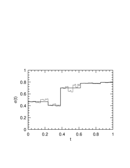
Figure 2: Three five step approximation (in black) to the limiting scaling function (in gray).

4 Simulations

To understand the sources of error in determining the scaling function, I will compute it from an orbit of a map that is not exactly at the golden mean rotation number but at one of its continued fraction approximants with a length typical of what is obtained in laboratory experiments. In particular I will consider the orbit with rotation number $21/34$, which in the circle map occurs at $\omega=0.606\,439$ on the critical line ($k=1$). To simulate the effects of noise fluctuations the control parameters $k$ and $\omega$ of the sine circle map will be slightly varied at each iteration. Both $k$ and $\omega$ will be replaced by

$$\begin{array}[]{lcr}k_{i}&=&k+r_{i}\Delta k\\ \omega_{i}&=&\omega+s_{i}\Delta\omega\end{array}\mbox{\ ,}$$ (10)

where $\Delta k$ and $\Delta\omega$ are the strength of the fluctuations and $r_{i}$ and $s_{i}$ are random numbers uniformly distributed in the interval from $-1$ to $1$. Notice that $k$ and $\omega$ remain fixed during the random process, and for the uniform distribution, represent the average values of $k_{i}$ and $\omega_{i}$. An orbit from the noisy sine circle map is generated by

$$x_{i+1}=x_{i}+\omega_{i}-\frac{k_{i}}{2\pi}\sin(2\pi x_{i})\mbox{\ .}$$ (11)

If the average parameter values are within the $21/34$ tongue, then the map is iterated a few hundred times before any orbit points are used to compute the scaling function. If the average parameters are not within the tongue, then the map is started at the inflection point.

The orbit is averaged according to the procedure proposed by Belmonte et al. [6], where points that are nearby in coordinate space are averaged together and coalesced into a single orbit point of an averaged periodic orbit. If the average parameter values of the map are within the tongue of the rotation number being considered, the group of points to be averaged can be unambiguously distinguished for errors as large as $\Delta k=\Delta\omega=0.05$, an error much larger than in most experiments. If the average parameter values are outside the tongue, then the number of groups to be averaged will depend on the length of the data set.

The first observation from the numerical simulations is that small errors can lead to largely distorted scaling functions. In figure 3a the scaling function for a short orbit ($21/34$) at parameters $k=0.9999$ and $\omega=0.6063$, which is close to the superstable point of the tongue, is compared with the theoretical curve. The amplitude of the error fluctuations are small ($\Delta k=\Delta\omega=10^{-4}$) which keeps the map parameters within the tongue. In this case there are large deviation from the theoretical curve. In figure 3b, for the same orbit length, the scaling function is computed with fluctuation noise 100 times larger, but with parameters ($k=1.0$ and $\omega=0.6066$) closer to the golden mean critical point. The difference between the scaling function obtained from the short orbit and the theoretical curve is smaller than in figure 3a. This at first seems paradoxical: the curve with larger fluctuations is closer to the theoretical curve than the curve with smaller fluctuations.

Figure 3: Different type of errors lead to different scaling functions. In both figures the theoretical curve is indicated by a solid line. In figure (a) the fluctuation errors are small, but the scaling function deviates largely from the theoretical curve. In figure (b) the fluctuation errors are large, but the scaling function deviates only slightly from the theoretical curve.

To quantify the differences between the theoretical and short period scaling function the $L^{1}$ norm can be used. This norm is proportional to the area in between both curves. If $\sigma(t)$ is the theoretical scaling function with five steps, and $\sigma_{o}(t)$ is the scaling function obtained from the orbit with $34$ points, also with five steps, then the error between them is defined as

$$e(\sigma,\sigma_{o})=\frac{1}{c_{o}}\int_{0}^{1}dt\,|\sigma(t)-\sigma_{o}(t)|\mbox{\ ,}$$ (12)

where $c_{0}$ is a normalization constant. The constant is chosen so that error between the theoretical scaling function and the one obtained from a short orbit at the irrational winding number is one. The constant $c_{0}$ is computed to be $0.01121$. With this norm the error between the curves in figure 3a is $2.26$ and between the the curves in figure 3b is $0.53$.

Figure 4: The error in approximating the scaling function by an orbit generated from a map with systematic error. The winding number $\omega$ is measured in units of the width of the $21/34$ tongue away from the golden mean and the error is the area in between the curves. The arrow shows the location of the point for the $21/34$ cycle

The systematic error constitute the larger source of error. This can be verified by plotting the error between the scaling function obtained at a point away from the golden mean rotation number and another point along the critical line. The further the rotation number is from the golden mean, the larger the difference between the two scaling functions. In figure 4 the inflection point is iterated for 34 times; from this orbit a five step scaling function is computed, which is then compared to the asymptotic five step scaling function. In the figure the rotation number is measured from its departure from the golden mean rotation number in units of the width of the $21/34$ tongue. In actual units of the map the horizontal axis ranges from $0.60638$ to $0.60685$, which is four times the width of the $21/34$ tongue. According to the plot, the error is smallest when the rotation number is closest to the golden mean, and increases as one departs from it on either side. The exact minimum in the error curve does not coincide with the golden mean because of finite size effects in computing the scaling function. For the error curve to be a smooth function of the rotation number it is necessary that all orbits start at the same point, the inflection point in this case.

The plot of figure 4 was obtained from iterating a map without fluctuations in the control parameters. One would expect the the results obtained without the error are those that would be obtained had the map with error been iterated and averaged a large number of times. This is the case if the points are averaged according to their time index, that is, for an orbit of period $P$, the average over the fluctuations of the $k$-th point of a periodic orbit are computed from

$$\langle x_{k}\rangle=\lim_{n\rightarrow\infty}\frac{1}{n}\sum_{1\leq i\leq n}x_{k+iP}\mbox{\ .}$$ (13)

But this may not be the average that is computed in an experiment. Sometimes it is simpler, or consistent with time delay coordinates, to average the points that are close to each other in time delay space (this was the procedure adopted in reference [6]). In table 1 an orbit for a map at the superstable point has been iterated with a small error ($\Delta k=\Delta\omega=10^{-3}$). The map is iterated while the parameters fluctuate. Each point is compared with the exact orbit and iterated points that come close to the same exact orbit point are averaged together. From the averaged orbit the five level approximation to the scaling function is computed and used to determine the error associated with the orbit by comparing it to the scaling function without noise. By “without noise”, I mean the scaling function that is obtained by iterating the map with the average parameters values of the simulation with noise. The table shows the results of longer and longer averages. At first the error diminishes, but as the number of samples increases the error appears to remain constant. The conclusion from the table is that one has to be careful that the limits involved in the averaging procedure are well defined and converge to ones expectations.

samples	error
$10^{0}$	$1.99065$
$10^{1}$	$0.21849$
$10^{2}$	$0.53230$
$10^{3}$	$0.49462$
$10^{4}$	$0.52383$
$10^{5}$	$0.51801$

Table 1: Error between the scaling function computed with and without noise. The noisy map has fluctuating parameters with average at the superstable point of the $21/34$ tongue. The averaging is done in coordinate space. As the number of samples increases the error does not go to zero, as would be expected.

5 Conclusions

From the numerical simulations one sees that even large errors can have little effect on the extraction of the universal scaling function, provided that the parameters of the system are well tuned to the golden mean rotation number at the transition to chaos, as can be seen from figure 3. The error in computing the scaling function depends on how close the parameters are to the transition point to chaos, a quantity that is difficult to control in experiments, as they are invariably subject to drift. The drift comes from the conflicting requirement of tuning the parameters to the smallest possible tongue (and therefore at the limit of instrumentation) and of obtaining the longest possible times series.

Also from the numerical simulations the perils of averaging the orbit in coordinate space where pointed out. The noise in the system causes the orbit to land close to the “wrong” group of points for its phase within the period, which leads to the non-convergence of the averaging procedure. I have no mathematical proof for this lack of convergence, but table 1 gives numerical evidence towards the result.

It hardly seems worthwhile to extract the scaling function given all these difficulties, specially given that the $f(\alpha)$ spectrum of singularities seems very robust to noise and simple to extract from experimental time series. It also appears to give an infinity of scales for the problem, just as the scaling function. The difficulty with this argument lies with the error bars of the spectrum of singularities. With error bars of the order of 1%, the spectrum of singularity is equivalent to just three of the values of the scaling function [17]; the spectrum of singularities does not give individual scales but mixes them all into one function. In order to extract further information from the spectrum of singularities the errors would have to be reduced well below the 1% level, which does not seem possible even in numerical simulations. Contrast this with the scaling function. There every different scaling (the $\sigma^{(n)}_{s}$) can be individually and independently extracted.

Scaling functions are the fundamental objects in the study of low dimensional dynamical systems, and it is surprising how little attention they have received in the literature, both theoretically and experimentally. If they are to be extracted from experimental time series new techniques will have to be developed to control the systematic errors.

References

- [1] N. H. Packard, J. P. Crutchfield, J. D. Farmer, and R. S. Shaw. Geometry from a time series. Physical Review Letters, 45:712 – 716, 1980.
- [2] Floris Takens. Detecting strange attractors in turbulence. In Lecture Notes in Mathematics 898, pages 366–381. Springer, Berlin, 1981.
- [3] Thomas C. Halsey, Mogens H. Jensen, Leo Kadanoff, Itamar Procaccia, and Boris I. Shraiman. Fractal measures and their singularities: the characterization of strange sets. Physical Review A, 33(2):1141–1151, February 1986.
- [4] Mitchell J. Feigenbaum. The transition to aperiodic behavior in turbulent systems. Communications of Mathematical Physics, 77:65 – 86, 1980.
- [5] Mitchell J. Feigenbaum, Mogens H. Jensen, and Itamar Procaccia. Time ordering and the thermodynamics of strange sets: Theory and experimental tests. Physical Review Letters, 57:1503–1506, 1986.
- [6] A. Belmonte, Michael J. Vinson, James A. Glazier, Gemunu H. Gunaratne, and Brian G. Kenny. Trajectory scaling functions at the onset of chaos: experimental results. Physical Review Letters, 61(5):539–542, 1988.
- [7] George A. Christos and Tony Gherghetta. Trajectory scaling function for the circle map the quasiperiodic route to chaos. Physical Review A, 44(2):898–907, July 1991.
- [8] D. Sullivan. Differentiable structures determined by fractal like sets, determined by intrinsic scaling functions on dual Cantor sets. In P. Zweifel, G. Gallavotti, and M. Anile, editors, Non-linear evolution and chaotic phenomena. Plenum, New York, 1987.
- [9] Mitchell J. Feigenbaum. Presentation functions and scaling function theory for circle maps. Nonlinearity, 1:577–602, 1988.
- [10] K. M. Khanin and Ya. G. Sinai. A new proof of M. Herman’s theorem. Communications of Mathematical Physics, 112:89–101, 1987.
- [11] R. Ecke, Ronnie Mainieri, and T. Sullivan. Universality in quasiperiodic Rayleigh-Bérnard convection. Physical Review A, 44(12):8103–8118, December 1991.
- [12] R.E. Ecke, Y. Maeno, H. Haucke, and J.C. Wheatley. Critical dynamics near the oscillatory instability in Rayleigh-Bénard convection. Physical Review Letters, 53:1567, 1984.
- [13] Y. Maeno, H. Haucke, R.E. Ecke, and J.C. Wheatley. Oscillatory convection in a dilute 3He-superfluid-4He solution. J. Low Temp. Phys., 59:305, 1985.
- [14] S. Ostlund et al. Universal properties of the transition from quasi-periodicity to chaos in dissipative systems. Physica D, 7:303–342, 1983.
- [15] M. Feigenbaum, L. P. Kadanoff, and S. J. Shenker. Quasiperiodicity in dissipative systems: a renormalization group analysis. Physica D, 5:370–386, 1982.
- [16] Ronald L. Graham, Donald E. Knuth, and Oren Patashnik. Concrete Mathematics. Addison-Wesley, Reading, 1989.
- [17] Mitchell J. Feigenbaum. Some characterizations of strange sets. Journal of Statistical Physics, 46:919–924, 1987.