Bayes linear adjustment for variance matrices

Abstract

We examine the problem of covariance belief revision using a geometric approach. We exhibit an inner-product space where covariance matrices live naturally — a space of random real symmetric matrices. The inner-product on this space captures aspects of our beliefs about the relationship between covariance matrices of interest to us, providing a structure rich enough for us to adjust beliefs about unknown matrices in the light of data such as sample covariance matrices, exploiting second-order exchangeability specifications.

Keywords: BELIEF ADJUSTMENT; COVARIANCE ESTIMATION; EXCHANGEABILITY; LINEAR BAYES; MATRIX INNER-PRODUCT; SUBJECTIVIST.

1 Revising beliefs about covariance structures

Quantifying relationships between variables is of fundamental importance in Bayesian analysis. However, there are many difficulties associated even with learning about covariances. For example, it is often difficult to make prior covariance specifications, but it is usually even harder to make the statements about the uncertainty in these covariance statements which are required in order to learn about the covariance statements from data. Further, a covariance structure is more than just a collection of random quantities, so we should aim to analyse such structures in a space where they live naturally. In this paper, we develop and illustrate such an approach, based around a geometric representation for variance matrices and exploiting second-order exchangeability specifications for them.

2 Current approaches to covariance estimation

Until recently, most authors have followed a Wishart conjugate prior approach (see for example, ?) or ?)). This approach, whilst tractable, places severe restrictions on the form of the prior distribution. More recently, a different approach has been proposed by ?), who learn about the log of the covariance matrix using data. This solves the positivity problems associated with covariance revision, but makes prior belief specification more difficult.

?), make further progress: working within a distributional Bayesian paradigm, they develop a reasonably flexible prior over the elements of a covariance structure, and offer interpretations for the parameters that one is required to specify. However, this work is still restricted to multivariate Normal likelihoods, and there is a weak restriction on the form of the mean structure for the data.

3 Bayes linear methods

The Bayes linear approach to subjective statistical inference makes expectation (rather than probability) primitive. An overview of the methodology is given in ?). In particular, as we are not forced to specify full prior measures over all variables of interest, we may exploit second-order exchangeability to allow us to construct statistical models directly from small numbers of belief specifications over observables. Foundational issues raised by Bayes linear analysis of exchangeable specifications are discussed in ?). We now show that these methods offer a simple and tractable approach to covariance estimation, linking sample covariance matrices with their “population” counterparts, in a natural geometric setting.

4 Exchangeable representations for covariances

Let $\underline{X}_{1},\underline{X}_{2},\ldots$ be an infinite, second-order exchangeable sequence of random vectors, each of length $r$, namely a sequence for which $\underline{X}_{k}=(X_{1k},\ldots,X_{rk})^{T}$, $\mu_{i}={\rm E}(X_{ik}),c_{ij}={\rm Cov}(X_{ik},X_{jk})$ does not depend on $k$, and $c_{ij}^{\prime}={\rm Cov}(X_{ik},X_{jl}),k\not=l$ does not depend on $k,l$.

From this specification, we may use the second-order exchangeability representation theorem [Goldstein (1986] to decompose $X_{ik}$ as

$$X_{ik}=M_{i}+R_{ik}$$ (1)

where ${\rm E}(R_{ik})={\rm Cov}(M_{j},R_{ik})={\rm Cov}(R_{ik},R_{jl})=0,\forall i,j,k\not=l$, and the vectors $\underline{R}_{k}=(R_{1k},\ldots,R_{rk})^{T}$ form a second order exchangeable sequence. Here, $M_{i}$ may be thought of as representing underlying population behaviour, and $R_{ik}$ as representing individual variation.

Consider the sequence of $\frac{r(r+1)}{2}$-dimensional vectors

$$\underline{Y}_{k}=(R_{1k}R_{1k},\ldots,R_{1k}R_{rk},R_{2k}R_{2k},\ldots,R_{2k}R_{rk},\ldots,\ldots,R_{rk}R_{rk})^{T}$$ (2)

representing the quadratic products of the residuals. Suppose that we assume that the $\underline{Y}_{k}$ are second-order exchangeable, and that we express the additional specifications $v_{ijpq}={\rm Cov}(R_{ik}R_{jk},R_{pk}R_{qk})$ and $v_{ijpq}^{\prime}=$ ${\rm Cov}(R_{ik}R_{jk},R_{pl}R_{ql}),k\not=l$. Then we may similarly decompose the elements of $\underline{Y}_{k}$ as

$$R_{ik}R_{jk}=V_{ij}+U_{ijk}$$ (3)

with properties as for representation (1). In particular ${\rm Cov}(U_{ijk},U_{pqk})=u_{ijpq}$ is not dependent on $k$. Here, $V_{ij}$ represents underlying covariance behaviour, and $U_{ijk}$ represents individual variation within the quadratic products of residuals.

If we observe a sample $\underline{X}_{1},\ldots,\underline{X}_{n}$ of size $n$, then sample covariances take the form

$$S_{ij} = \frac{1}{n-1}\sum_{w=1}^{n}(X_{iw}-X_{i\cdot})(X_{jw}-X_{j\cdot})$$ (4)

$$= \frac{1}{n-1}\sum_{w=1}^{n}(R_{iw}-R_{i\cdot})(R_{jw}-R_{j\cdot})$$ (5)

Beliefs over the sample covariances $S_{ij}$ are, by (5), uniquely determined by representation (3), and can be written

$$S_{ij}=V_{ij}+T_{ij}$$ (6)

where $V_{ij}$ is as in (3), ${\rm E}(T_{ij})=0$ and ${\rm Cov}(V_{ij},T_{ij})=0$. The covariance structure over $T_{ij}$ is given by

$${\rm Cov}(T_{ij},T_{pq})=\frac{u_{ijpq}}{n}.$$ (7)

Observing sample covariances from a sample of size $n$ reduces uncertainty for $V_{ij}$, the underlying covariance values, but is uninformative for the $U_{ijk}$ for $k>n$.

Let $S$ be the matrix whose $(i,j)$th element is $S_{ij}$, and define $V$ and $T$ similarly. We then have

$$S=V+T$$ (8)

5 Geometric representation for random matrices

We now develop the representation which will allow us to treat a covariance matrix as a single object. Let $B=[B_{1},B_{2},\ldots]$ be a collection of random $r\times r$ real symmetric matrices, representing unknown matrices of interest to us. These might, for example, represent population covariance matrices. Let $D=[D_{1},D_{2},\ldots]$ be another such collection, representing observable matrices (such as sample covariance matrices). Finally, let $C=[C_{1},C_{2},\ldots]$ be a basis for the space of constant $r\times r$ real symmetric matrices. We now form a vector space

$$L=span\{B\cup C\cup D\}$$ (9)

of all linear combinations of the elements of these collections, and define the inner-product (over equivalence classes) on $L$ as

$$(P,Q)={\rm E}({\rm Tr}(PQ))\quad\forall P,Q\in L$$ (10)

which induces the metric

$$d(P,Q)^{2}={\rm E}(\|P-Q\|_{F}^{2})\quad\forall P,Q\in L,$$ (11)

where $\|\cdot\|_{F}$ denotes the Frobenius norm of a matrix. This is the sum of the squares of the elements, or equivalently, the sum of the squares of the eigenvalues. Where necessary, we form the completion of the space. The (complete) inner-product space is denoted by $M$.

Analogously with the revision of belief over scalar quantities [Goldstein (1981], we learn about the elements of the collection $B$, by orthogonal projection into subspaces of $M$ spanned by elements of the collection $C\cup D$, in order to obtain the corresponding adjusted expectations, namely the linear combinations of sample covariance matrices which give our adjusted beliefs.

If all matrices of interest contain only one non-zero component (all in the same position), the inner product becomes $(P,Q)={\rm E}(P_{ij}Q_{ij})$, inducing the distance $d(P,Q)^{2}={\rm E}((P_{ij}-Q_{ij})^{2})$, as for the usual Bayes linear theory for scalar quantities. The matrix structure is a generalisation of the scalar Bayes linear structure, and scalar Bayes linear adjustments can be recovered by decomposing all variance structures to the one component level.

The matrices we are considering do not have to be finite dimensional. All of the theory remains valid if we think in terms of representations of random linear self-adjoint operators on a (possibly infinite-dimensional) vector space.

6 Decomposing the variance structure

As a simple example, $B$ might consist only of the “population” covariance matrix, $V$ for a particular problem, and $D$ might be the corresponding sample covariance matrix, $S$, based on $n$ observations. In this case, our adjusted expectation for the “population” matrix would be a weighted linear combination of the prior and sample covariance matrices. However, by breaking down the sample covariance matrix into its component sub-matrices, we may resolve a greater proportion of our uncertainty about the “population” covariance matrix.

For simplicity, consider the case where we wish to learn about the covariance structure induced by representation (3) for $2$-dimensional vectors. The covariance matrices will be $2\times 2$. Consider the sample covariance matrix

$$S=\left(\begin{array}[]{cc}S_{11}&S_{12}\\ S_{12}&S_{22}\end{array}\right)$$ (12)

and the corresponding “population” covariance matrix

$$V=\left(\begin{array}[]{cc}V_{11}&V_{12}\\ V_{12}&V_{22}\end{array}\right)$$ (13)

In the notation of the previous section, we could restrict ourselves to

$$B=[V],D_{S}=[S],C=\left[\left(\begin{array}[]{cc}1&0\\ 0&0\end{array}\right),\left(\begin{array}[]{cc}0&1\\ 1&0\end{array}\right),\left(\begin{array}[]{cc}0&0\\ 0&1\end{array}\right)\right],$$ (14)

where all $2\times 2$ matrices can be constructed as linear combinations of the elements of $C$. Using these collections, our adjusted expectation for $V$ given $D_{S}$ would take the form

$${\rm E}_{D_{S}}(V)=(1-\alpha){\rm E}(V)+\alpha S$$ (15)

where $\alpha$ is the coefficient of the orthogonal projection determined by the inner-product (10). Explicitly:

$$\alpha = \frac{(V-{\rm E}(V),V-{\rm E}(V))}{(S-{\rm E}(S),S-{\rm E}(S))}$$ (16)

$$= \frac{\sum_{i=1}^{2}\sum_{j=1}^{2}n{\rm Var}(V_{ij})}{\sum_{i=1}^{2}\sum_{j=1}^{2}\{n{\rm Var}(V_{ij})+{\rm Var}(U_{ij})\}}$$ (17)

However, to improve the precision of our estimates, our projection space could be enlarged by constructing

$$D_{I}=\left[\left(\begin{array}[]{cc}S_{11}&0\\ 0&0\end{array}\right),\left(\begin{array}[]{cc}0&S_{12}\\ S_{12}&0\end{array}\right),\left(\begin{array}[]{cc}0&0\\ 0&S_{22}\end{array}\right)\right]$$ (18)

We call such a space the individual variance collection. This allows different sample covariances to have different weights, if for example, we have higher prior uncertainty about some of the variances. Indeed, we may take this a stage further, and construct

$$D_{C} = \left[\left(\begin{array}[]{cc}S_{11}&0\\ 0&0\end{array}\right),\left(\begin{array}[]{cc}0&S_{11}\\ S_{11}&0\end{array}\right),\left(\begin{array}[]{cc}0&0\\ 0&S_{11}\end{array}\right),\right.$$ (39)

$$\left(\begin{array}[]{cc}S_{12}&0\\ 0&0\end{array}\right),\left(\begin{array}[]{cc}0&S_{12}\\ S_{12}&0\end{array}\right),\left(\begin{array}[]{cc}0&0\\ 0&S_{12}\end{array}\right),$$

$$\left.\left(\begin{array}[]{cc}S_{22}&0\\ 0&0\end{array}\right),\left(\begin{array}[]{cc}0&S_{22}\\ S_{22}&0\end{array}\right),\left(\begin{array}[]{cc}0&0\\ 0&S_{22}\end{array}\right)\right]$$

We call this last collection the complete variance collection. This not only allows the different covariances to have different weights, but also allows relationships between covariances to have an effect on the adjustment. If we project $V$ into $D_{C}$, then our adjusted expectation for $V$ will correspond precisely with the adjustment which would have been obtained using Bayes linear estimation on the quadratic products of the residuals in the scalar space.

We can break down the population matrix in the same way if necessary. In particular, we let

$$V_{I}=\left[\left(\begin{array}[]{cc}V_{11}&0\\ 0&0\end{array}\right),\left(\begin{array}[]{cc}0&V_{12}\\ V_{12}&0\end{array}\right),\left(\begin{array}[]{cc}0&0\\ 0&V_{22}\end{array}\right)\right].$$ (40)

As we enlarge the projection space, we resolve more of our uncertainty about the variance structures, at the expense of doing more work. Generally we should project into as rich a space as is practicable, but for large variance matrices, the difference both in computational effort and in effort required for prior specification, between adjusting by $D_{S}$, $D_{I}$ and $D_{C}$ is substantial, so that we must make a subjective assessment of the relative benefits of each adjustment.

7 Example

7.1 Examination performance

We are currently investigating the examination performance of first year mathematics undergraduate students at Durham university. We are particularly interested in those students who have only one A Level in mathematics, and so we restrict attention to these in our account. For illustrative purposes, we focus on a few key variables, namely a summary of A Level performance ($A$), performance in the Christmas exams ($C$), and the end of year exam average ($E$).

For the exchangeable decomposition of (say) $A_{k}$, we will write

$$A_{k}=M_{A}+R_{A_{k}}$$ (41)

and for the exchangeable decomposition of (say) $R_{A_{k}}R_{C_{k}}$, we write

$$R_{A_{k}}R_{C_{k}}=V_{AC}+U_{AC_{k}}$$ (42)

so that, for example, $V_{AC}$ represents the underlying covariance between the $A$ and $C$ variables, and $U_{AC_{k}}$ represents the residual for the $k$th observation. We construct the “population” and sample covariance matrices:

$$V=\left(\begin{array}[]{ccc}V_{AA}&V_{AE}&V_{AC}\\ V_{AE}&V_{EE}&V_{EC}\\ V_{AC}&V_{EC}&V_{CC}\end{array}\right),\quad S=\left(\begin{array}[]{ccc}S_{AA}&S_{AE}&S_{AC}\\ S_{AE}&S_{EE}&S_{EC}\\ S_{AC}&S_{EC}&S_{CC}\\ \end{array}\right)$$ (43)

A conditional linear independence graph [Goldstein (1990] was formed to represent beliefs about the relationships between the quadratic products of the residuals (Figure 1). The common variance node reflects beliefs about the positive correlation between variances. Covariances are influenced by the corresponding variances. This graph was used to help structure the belief specification over the mean components of the variance structure.

Figure 1: A conditional linear independence graph for the mean components of the quadratic products of the residuals

Specifications are also required over the residual components of the variance structure. These specifications are more difficult to make, since we are not used to thinking about such quantities. In this example, for simplicity, our belief specifications over the residual structure were chosen to be consistent with those imposed under a multivariate normal specification corresponding to our prior specifications over the elements $R_{ik}$. Having made specifications over the quadratic products of residuals, beliefs over all relevant covariance matrices are now determined.

From the sample covariance matrix, $S=D_{S}$, we construct the individual variance collection, $D_{I}$ ($6$ objects) and the complete variance collection, $D_{C}$ ($36$ objects), as well as the individual collection for the mean structure, $V_{I}$ ($6$ objects). We form the random matrix space, $M$ over all these objects, and investigate adjustments in this space.

7.2 Quantitative analysis

The prior covariance matrix was specified directly as follows:

$${\rm E}(V)=\left(\begin{array}[]{rrr}7.98&11.14&15.75\\ 11.14&56.26&53.04\\ 15.75&53.04&100.00\end{array}\right)$$ (44)

The sample covariance matrix (34 cases) is:

$$S=\left(\begin{array}[]{rrr}8.28&20.15&24.75\\ 20.15&178.30&160.74\\ 24.75&160.74&258.26\end{array}\right)$$ (45)

The adjusted matrices were formed as the appropriate linear combinations of the observables, as described in section 5, and derived explicitly for the simplest case in section 6.

$${\rm E}_{D_{S}}(V) = \left(\begin{array}[]{rrr}8.08&14.08&18.69\\ 14.08&96.08&88.18\\ 18.69&88.18&151.65\end{array}\right)$$ (49)

$${\rm E}_{D_{I}}(V) = \left(\begin{array}[]{rrr}8.04&15.96&17.72\\ 15.96&98.90&78.63\\ 17.72&78.63&159.21\end{array}\right)$$ (53)

$${\rm E}_{D_{C}}(V) = \left(\begin{array}[]{rrr}8.30&15.43&20.06\\ 15.43&92.04&80.66\\ 20.06&80.66&156.79\end{array}\right)$$ (57)

These adjusted matrices may be used as a basis for assessing our posterior beliefs about the matrix object [Goldstein (1994].

Note that the last matrix (57) represents the adjusted matrix which would have been obtained using a standard Bayes linear analysis on the quadratic products of the residuals. In this particular example, all adjusted matrices are positive definite. In general, we view negative eigenvalues in the revised structure as providing diagnostic warnings of possible conflicts between prior beliefs and the data.

We would like to be able to compare the estimates of $V$: ${\rm E}_{D_{C}}(V)$, ${\rm E}_{D_{S}}(V)$, and ${\rm E}_{D_{I}}(V)$. Thus, we use the standard interpretive and diagnostic features of the Bayes linear methodology to assess the model and understand the adjustments taking place.

7.3 Bayes linear influence diagram

Figure 2 shows a Bayes linear influence diagram representing the adjustments and corresponding diagnostic information for the random matrices. Such diagrams are described in detail in ?) for random quantities, with a similar interpretation for random matrices, where conditional linear independence is determined instead by the inner-product (10), so that conditional linear independence becomes

$$B\amalg C/D\iff{\rm E}[{\rm Tr}\{(B-{\rm E}_{D}(B))(C-{\rm E}_{D}(C))\}]=0$$ (58)

as described in ?).

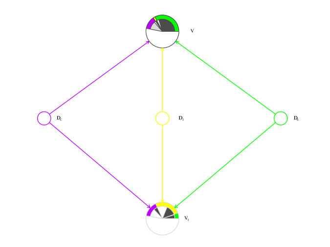
Figure 2: Diagnostic influence diagram summarising changes in expectation of the matrix objects

The outer shadings of the $V$ node represent proportions of uncertainty about $V$ resolved by projection into the various spaces. Shadings start at 3 o’clock, and progress in an anti-clockwise fashion. The full circle represents the total uncertainty about the value of the covariance matrix. The first outer portion shaded represents the proportion of our uncertainty resolved by the sample covariance matrix alone ($D_{S}$). By comparing this with the first shaded portion for the $V_{I}$ node, we see that we have learned considerably more about the matrix object, than we have about the 6-dimensional space over the individual variance collection.

The next shading gives the additional information gained by using the individual collection as the projection space. We see that this tells us a great deal more about the elements of the $V_{I}$ collection, but little about the matrix object as a whole. The other shading shows the additional uncertainty resolved due to including the complete variance collection in our projection space. We see that there is information to be gained by enriching our projection space, but we must balance information gained with extra effort involved. Whether or not we choose to include the complete variance collection will depend upon the size of the problem under consideration, and upon how much the answer really matters.

Shadings in the centres of the nodes are diagnostics based on the size and bearing of the adjustments, as described in ?). We generalise the bearing to the space of random matrices as follows: For any given constant matrix, $G$, and projection space $D$, the bearing is defined to be the unique random matrix, $B$, with the property

$$(A-{\rm E}(A),B)=({\rm E}_{d}(A),G)-({\rm E}(A),G),\ \forall A\in M$$ (59)

where ${\rm E}_{d}(A)$ represents the realisation of ${\rm E}_{D}(A)$ after observing $D=d$. Different choices of the constant matrix, $G$, give information about different projections of the adjusted expectations. The choice of $G$ which causes diagnostics to match up exactly with those for scalar Bayes linear adjustment in the case where we are dealing exclusively with one-component matrices, is the choice given by the constant matrix whose elements are all $1$. At the centre of the $V$ node, dark (light) shadings represent changes in expectation larger (smaller) than we expected a priori. We can see that adjusting by the sample covariance matrix, $D_{S}$, caused a much larger change in expectation than we expected a priori. This is evidence that we were too confident about our ability to predict the true value of the covariance matrix, and suggests that we should re-examine the prior specification. We also notice that adding the complete variance collection, $D_{C}$, to the adjustment had the potential to change our expectation considerably, but in fact, hardly changed it at all. This is perhaps evidence that we overestimated the importance of the covariance terms.

8 Summary

Analysing matrices in a space where they live naturally not only has great aesthetic appeal, but is very powerful and illuminating in practice. Working in this space simplifies the handling of large matrices, by reducing the number of quantities involved and summarising effects over the whole covariance structure. For the same reasons, diagnostic information about adjusted beliefs is easier to interpret. We may decompose structures as much or as little as we wish.

This approach allows us to learn about collections of covariance structures, and examine their relationships. It generalises the “element by element” approach to revision, which can be viewed as taking place in a subspace of the larger space. Exchangeability representations lie at the heart of the methodology: all of our specifications are over observables, or quantities constructed from observables, rather than artificial model parameters, and we make no distributional assumptions for the data or the prior.

9 Acknowledgements

The first named author is supported by a grant from the UK’s EPSRC. All computations, and the production of the diagnostic influence diagram, were carried out using the Bayes linear computing package, [B/D] , outlined in ?), and explained in detail in ?). The comments from an anonymous referee have helped us improve the clarity of this paper.

References

- Brown, Le, and Zidek (1994 Brown, P., N. Le, and J. Zidek (1994). Inference for a covariance matrix. In P. Freeman and A. Smith (Eds.), Aspects of Uncertainty: A Tribute to D.V. Lindley, pp. 77–92. Wiley.
- Chen (1979 Chen, C. (1979). Bayesian inference for a normal dispersion matrix. J. Roy. Statist. Soc. Ser. B 41, 235–248.
- Farrow and Goldstein (1993 Farrow, M. and M. Goldstein (1993). Bayes linear methods for grouped multivariate repeated measurement studies with application to crossover trials. Biometrika 80(1), 39–59.
- Goldstein (1981 Goldstein, M. (1981). Revising previsions: a geometric interpretation. J. R. Statist. Soc. B:43, 105–130.
- Goldstein (1986 Goldstein, M. (1986). Exchangeable belief structures. J. Amer. Statist. Ass. 81, 971–976.
- Goldstein (1988 Goldstein, M. (1988). The data trajectory. In J.-M. Bernardo et al. (Eds.), Bayesian Statistics 3, pp. 189–209. Oxford University Press.
- Goldstein (1990 Goldstein, M. (1990). Influence and belief adjustment. In J. Smith and R. Oliver (Eds.), Influence Diagrams, Belief Nets and Decision Analysis. Chichester: Wiley.
- Goldstein (1994 Goldstein, M. (1994). Revising exchangeable beliefs: subjectivist foundations for the inductive argument. In P. Freeman and A. Smith (Eds.), Aspects of Uncertainty: A Tribute to D. V. Lindley. Wiley.
- Goldstein, Farrow, and Spiropoulos (1993 Goldstein, M., M. Farrow, and T. Spiropoulos (1993). Prediction under the influence: Bayes linear influence diagrams for prediction in a large brewery. The Statistician 42(2), 445–459.
- Goldstein and Wooff (1995 Goldstein, M. and D. Wooff (1995). Bayes linear computation: concepts, implementation and programming environment. Statistics and Computing, to appear.
- Haff (1980 Haff, L. (1980). Empirical bayes estimation of the multivariate normal covariance matrix. Ann. Statist. 8, 586–597.
- Leonard and Hsu (1992 Leonard, T. and J. Hsu (1992). Bayesian inference for a covariance matrix. Ann. Statist. 20, 1669–1696.
- Wooff (1992 Wooff, D. (1992). [B/D] works. In J.-M. Bernardo et al. (Eds.), Bayesian Statistics 4, pp. 851–859. Oxford University Press.