A magnetic tomography of a cavity state

Abstract

A method to determine the state of a single quantized cavity mode is proposed. By adiabatic passage the quantum state of the field is transfered completely onto an internal Zeeman sub-manifold of an atom. Utilizing a method of Newton and Young (Ann. Phys. 49, 393 (1968)), we can determine this angular momentum state uniquely, by a finite number of magnetic dipole measurements with Stern-Gerlach analyzers. An example illustrates the influence of dissipation.

PACS Nos. 42.50.-p, 42.50Vk

The state of a quantum mechanical system is completely specified by its density operator ${\hat{\rho}}$. It is a fundamental as well as an important practical question of quantum mechanics to devise measurement schemes which allow a complete determination of ${\hat{\rho}}$. By a sequence of repeated measurements on an ensemble of identically prepared systems the state has to be characterized operationally. In quantum optics this topic of complete state determination has received recently considerable attention in the context of characterizing nonclassical states of the radiation field, and states of atomic and molecular motion [1, 2, 3, 4, 5, 6, 7, 8, 9, 10].

In a seminal paper, Vogel and Risken [1] have pointed out that the state of a single mode of the radiation field (equivalent to a one-dimensional harmonic oscillator) can be found by a tomographic techniques and corresponding experiments have been performed by Raymer and coworkers [2]. The central idea of quantum state tomography is based on a reconstruction of the density matrix ${\hat{\rho}}$ from measured quadrature probabilities $p_{x}(\theta)=(x,\theta|{\hat{\rho}}|x,\theta)$. Here $|x,\theta)$ is a rotated eigenstate of the quadrature operator ${\bf x}_{\theta}$, i.e $|x,\theta)={\cal R}(\theta)^{\dagger}\,|x\rangle=e^{i\theta{\bf a}^{\dagger}{\bf a}}\,|x\rangle$ with $\bf a$ and ${\bf a}^{\dagger}$ lowering and raising operators of the oscillator. Alternative schemes have been discussed in the literature under the name of state endoscopy [6] or by introducing discrete Wigner-functions [7]. Very recently, ideas were developed for a state determination of ions moving in harmonic trapping potentials [5, 10].

In the present paper we discuss a new scheme to measure the density matrix of the radiation field of a single quantized cavity mode by a magnetic tomography. It is based on combining ideas we have developed in the context of quantum state engineering of arbitrary Fock-state superpositions in a cavity by adiabatic passage [11], with a tomography of atomic angular momentum states by Stern-Gerlach measurements originally proposed in [12].

It is well know that the adiabatic change of a Hamiltonian interaction transforms initial energy-eigenstates into eigenstates of the final Hamilton operator [13]. This method to map quantum states is applied in various contexts of molecular- and atomic physics [11, 14, 15]. It is also the key mechanism for transferring the state of a quantized cavity mode onto the internal state manifold of an atom.

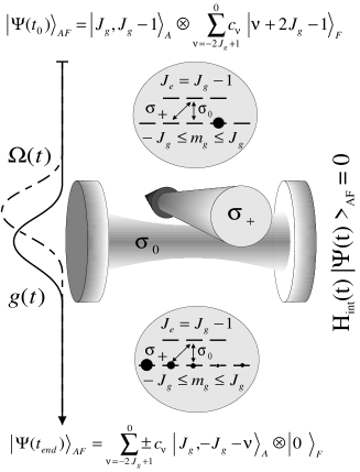
FIG. 1.: Evolution of a degenerate two level atom (angular momentum: $J_{g}\rightarrow J_{e}=J_{g}-1$) coupled to a quantized $\sigma_{0}$-polarized cavity mode. First, it passes through the profile a classical beam ($\sigma_{+}$) and then, with a delay, through the cavity.

According to Fig. 1, an atom passes adiabatically [11, 15] through the spatial profile of a classical $\sigma_{+}$-polarized laser beam [Rabi-frequency: $\Omega(t)$] and, with a spatio-temporal displacement $\tau>0$ , through the profile of a quantized, $\pi$-polarized cavity mode [atom-cavity coupling: $g(t-\tau)$]. We assume that the electronic structure of the atoms corresponds to an optical $J_{g}\rightarrow J_{e}=J_{g}-1$ dipole transition.

The coupled atom-cavity system evolves according to the time-dependent Hamiltonian

$$H(t)/\hbar=\omega_{c}\,a_{c}^{\dagger}a_{c}+\omega_{\rm eg}\sum_{m_{e}=-J_{e}}^{J_{e}}|J_{e},m_{e}\rangle_{A}\langle J_{e},m_{e}|_{A}+$$ (1)

$$\mbox{}-i\Omega(t)(e^{i\omega_{L}t}A_{1}-A_{1}^{\dagger}e^{-i\omega_{L}t})+ig(t-\tau)(a^{\dagger}A_{0}-A_{0}^{\dagger}a),$$ (2)

where $a_{c}$ and $\omega_{c}$ is the annihilation operator and oscillation frequency of the cavity mode, respectively. In terms of atomic basis states and Clebsch-Gordan coefficients $C_{\sigma,m_{g},m_{e}}^{1,J_{g},J_{e}}$, the atomic de-excitation operators $A_{0},A_{1}$ are defined by

$$A_{\sigma}=\sum_{|m_{g}|\leq J_{g},|m_{e}|\leq J_{e}}|J_{g},m_{g}\rangle_{A}\langle J_{e},m_{e}|_{A}C_{\sigma,m_{g},m_{e}}^{1,J_{g},J_{e}}.$$

The state space spanned by this Hamiltonian has the remarkable feature that it can be decomposed into invariant sub-spaces ${\cal H}=\bigoplus_{\nu=-2J_{g}}^{\infty}{\cal H}^{\nu}$. Due to angular momentum conservation, it is only possible to couple angular momentum states to a finite number of photon states by means of a unitary evolution (Eq. 1).

$${\cal H}^{\nu} = \left\{|m_{g}|\leq J_{g},0\leq n=\nu+J_{g}+m_{g}\right\|$$

$$\left.|J_{g},m_{g}\rangle_{A}\otimes|n\rangle_{C},|J_{e},m_{g}\rangle_{A}\otimes|n-1\rangle_{C}\right\}.$$

One element of the sub-space ${\cal H}^{\nu}$ is of particular interest, i.e. a linear combination involving only ground states [14, 16]

$$|\phi^{\nu}_{0}\rangle=\sum^{J_{g}-1}_{m_{g}=-J_{g}}\alpha_{m_{g}}^{\nu}|J_{g},m_{g}\rangle_{A}\otimes|\nu+J_{g}+m_{g}\rangle_{C}.$$ (3)

By an appropriate choice of coefficients $\alpha_{m_{g}}^{\nu}$,i.e.

$$\frac{\alpha_{m_{g}-1}^{\nu}(t)}{\alpha_{m_{g}}^{\nu}(t)} = \frac{g(t-\tau)}{\Omega(t)}\sqrt{\nu+J_{g}+m_{g}}\,\frac{C^{1,J_{g},J_{e}}_{0,m_{g},m_{g}}}{C^{1,J_{g},J_{e}}_{1,m_{g}-1,m_{g}}},$$ (4)

this normalized state ($\alpha_{J_{g}-1}^{\nu}={\cal N}$) becomes also an eigenvector of the Hamilton operator in the interaction representation (derived from Eq. (1)) and has a zero eigenvalue. According to the adiabatic theorem [13], this eigenvector approaches a stationary eigenstate of the corresponding Schrödinger-equation, if the time dependent change of the Hamilton operator during the total interaction time $T$ is much less than the characteristic transition frequencies ($\Omega_{\rm max}T$, $\sqrt{N_{\rm max}}g_{\rm max}T\gg 1$). Furthermore, if the delay and shape of the pulse sequences are chosen such that

$$0\stackrel{{\scriptstyle-\infty\leftarrow t}}{{\longleftarrow}}g(t-\tau)/\Omega(t)\stackrel{{\scriptstyle t\rightarrow+\infty}}{{\longrightarrow}}\infty,$$ (5)

then this is a mapping process that only permutes states up to a sign change $s_{\nu}=\mbox{sign}(\alpha_{-J_{g}-\nu}^{\nu}(+\infty))$.

$$|J_{g},J_{g}-1\rangle_{A}\otimes|\nu+2J_{g}-1\rangle_{C}\stackrel{{\scriptstyle-\infty\leftarrow t}}{{\longleftarrow}}|\phi^{\nu}_{0}(t)\rangle,$$

$$|\phi^{\nu}_{0}(t)\rangle\stackrel{{\scriptstyle t\rightarrow+\infty}}{{\longrightarrow}}s_{\nu}\,|J_{g},-J_{g}-\nu\rangle_{A}\otimes|0\rangle_{C}.$$

In other words, a coupled atom-cavity density operator ${\hat{\rho}}^{(AC)}$ that can be factorized initially into a pure atomic state and a field state containing less than $2J_{g}$ photons will be mapped to a product of atomic ground state superpositions and the cavity vacuum

$$|J_{g},J_{g}-1\rangle_{A}\langle J_{g},J_{g}-1|_{A}\otimes{\hat{\rho}}^{(C)}\stackrel{{\scriptstyle-\infty\leftarrow t}}{{\longleftarrow}}{\hat{\rho}}^{(AC)}(t)$$ (6)

$${\hat{\rho}}^{(AC)}(t)\stackrel{{\scriptstyle t\rightarrow+\infty}}{{\longrightarrow}}{\hat{\rho}}^{(A)}\otimes|0\rangle_{C}\langle 0|_{C},$$ (7)

with

$\displaystyle{\hat{\rho}}^{(C)}=\sum_{\nu,\mu=-(2J_{g}-1)}^{0}\rho_{\nu,\mu}^{(C)}\,|\nu+2J_{g}-1\rangle_{C}\langle\mu+2J_{g}-1|_{C},\\$

and

$\displaystyle{\hat{\rho}}^{(A)}=\sum_{\nu,\mu=-(2J_{g}-1)}^{0}s_{\nu}s_{\mu}\,\rho_{\nu,\mu}^{(C)}\,|-J_{g}-\nu\rangle_{A}\langle-J_{g}-\mu|_{A}.$

With reverse adiabatic passage, an internal atomic state is prepared uniquely by reading out the cavity state.

The complete characterization of such an angular momentum state by a number of magnetic dipole measurements was described in Ref. [12]. It requires to detect a set of physical observables that are proportional to

$\displaystyle\{|m|\leq J,|s|\leq 2J\,\|{\hat{P}}_{m}(\theta,\varphi_{s})\}.$

Here ${\hat{P}}_{m}(\theta,\varphi_{s})$ represents the projector onto a rotated state $|J,m,{\cal R}(\theta,\varphi_{s}){\vec{e}}_{z}\rangle=D^{(J)}({\cal R})\,|J,m,{\vec{e}}_{z}\rangle$, $s$ enumerates an arbitrary set of 4J+1 azimuthal angles $\varphi_{s}$ and $\theta$ is a constant inclination. This method can be implemented, for example, by the unitary evolution of an angular momentum state in a homogeneous magnetic field ${\vec{B}}(\theta,\varphi_{s})=|B|\,{\vec{n}}(\theta,\varphi_{s})$ oriented differently, each time the measurement is performed, and by using a conventional Stern-Gerlach analyzer Fig. 2.

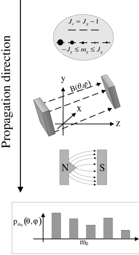
FIG. 2.: Setup of a Stern-Gerlach experiment with an additional homogeneous magnetic field ${\vec{B}}(\theta,\varphi)=|B|\,{\vec{n}}(\theta,\varphi)$ inducing spin precession around the axis ${\vec{n}}(\theta,\varphi)$

From the $J$-dimensional representation of the rotation group $D^{(J)}({\cal R})$ or the Wigner matrices $d^{(J)}(\theta)$ [17], one finds

$$|J,m,{\cal R}(\theta,\varphi){\bf e}_{z}\rangle = \sum_{n=-J}^{J}e^{-in\varphi}d^{(J)}_{nm}(\theta)\,|J,n,{\bf e}_{z}\rangle.$$ (8)

Hence, the occupation probabilities are given by

$$p_{m}(\theta,\varphi_{s})=\sum_{n,l=-J}^{J}e^{-i(n-l)\varphi_{s}}d^{(J)}_{nm}(\theta)d^{(J)}_{lm}(\theta)\,\rho_{ln}$$ (9)

This linear equation relates density matrix elements ($(2J+1)(2J+1)$ real numbers) to measured probabilities that are positive numbers. By determining $(2J+1)(4J+1)$ different probabilities, this seemingly over determined set of linear equations has a unique solution that is positive definite. For $|l|\leq J$, $0\leq w\leq J-l$, one finds

$$\rho_{l,l+w}=\sum_{m=-J}^{J}\sum_{j=0}^{2J}C_{m,-m,0}^{JJj}C_{l+w,-l,w}^{JJj}\frac{(-1)^{l-m}}{d_{w,0}^{(j)}(\theta)}X(\theta)_{wm}.$$ (10)

In case of an equally spaced array of azimuthal angles $\varphi_{s}$, i.e, $-\pi<\varphi_{s}=s\frac{2\pi}{4J+1}<\pi$, $|s|\leq 2J$, the quantity $X(\theta)$ is the discrete Fourier transform of the measured probability tableau

$$X(\theta)_{wm}=\frac{1}{4J+1}\sum_{s=-2J}^{2J}e^{iw\varphi_{s}}p_{m}(\theta,\varphi_{s}).$$ (11)

In contrast to systems with continuous degrees of freedom, the reconstruction algorithm of Eq. (10) is faithful if inclination angles $\theta$ are avoided where $d^{(J)}_{w,0}(\theta)$ vanishes (i.e. the zeros of an associated Legendre polynomial). Most detrimental to this state tomography is the loss of cavity photons during the adiabatic interaction. In contrast, spontaneous atomic decay is of minor importance as the adiabatic eigenstate is formed by a ground state superposition. To examine the influence of dissipation, we have coupled the atom-cavity system to an environment [11] and obtained the following master equation for the density operator ${\hat{\rho}}$.

$$\frac{d}{dt}\rho=-\frac{i}{\hbar}[H_{\rm eff}\rho-\rho H_{\rm eff}^{\dagger}]+\Gamma\sum_{\sigma=0,\pm 1}A_{\sigma}\rho A_{\sigma}^{\dagger}+\kappa\,a_{c}\rho a_{c}^{\dagger},$$ (12)

where $\Gamma$ and $\kappa$ denote the spontaneous decay rate and the inverse cavity life time, respectively.

In the interaction picture representation (derived from Eq. 1), the effective, non-hermitian Hamiltonian, introduced above, is given by

$$H_{\rm eff} = (\Delta-i\frac{\Gamma}{2})\sum_{m_{e}=-J_{e}}^{J_{e}}|J_{e},m_{e}\rangle\langle J_{e},m_{e}|-i\frac{\kappa}{2}\,a_{c}^{\dagger}a_{c}+$$ (14)

$$\mbox{}-i\Omega(t)(A_{1}-A_{1}^{\dagger})+ig(t-\tau)(a_{c}^{\dagger}A_{0}-A_{0}^{\dagger}a_{c}).$$

For simplicity, it is assumed that the cavity and the external laser have a common frequency $\omega_{c}=\omega_{L}$ and are detuned from the atomic resonance by $\Delta=\omega_{\rm eg}-\omega_{L}$. The resulting atomic density operator can be determined either by solving the master-equation (Eq. (12)) or alternatively, by averaging over a number of simulated quantum trajectories [18].

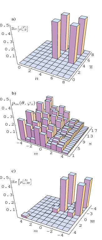
FIG. 3.: a) Real part of the initial cavity density matrix $\rho_{n,{\overline{n}}}^{(F)}$ vs. photon number $n,{\overline{n}}$; b) atomic ground state occupation probabilities $p_{m}(\theta,\varphi_{s})$ vs. magnetic quantum number $m$ and azimuthal phase index $s$ of an atom that moved adiabatically through the cavity; c) atomic density matrix $\rho_{m,{\overline{m}}}^{(A)}$ vs. magnetic quantum number $m,{\overline{m}}$, inverted tomographically from the data represented in Fig. 3b (see text for parameters).

In Fig. 3, the results of the mapping and reconstruction process are shown for an initially pure cavity state

$$|\psi(t_{0})\rangle_{C}=\frac{1}{\sqrt{2}}(|4\rangle_{C}+|7\rangle_{C}),$$ (15)

The real part of the initial cavity density matrix, i.e. $\rho^{(C)}(t_{0})=|\psi(t_{0})\rangle_{C}\langle\psi(t_{0})|_{C}$ vs. photon number $n,{\overline{n}}$ is shown in Fig. 3a. In order to map this cavity state onto a Zeeman submanifold, we assumed a sufficiently large degeneracy ($J_{g}=4\rightarrow J_{e}=3$). Both fields are tuned to the atomic resonance $\Delta=0$. All frequencies are scaled to the spontaneous decay rate of the atomic excited state $\Gamma$, as the peak Rabi-frequency $\Omega_{\rm max}=50\,\Gamma$ and the maximal cavity coupling constant $g_{\rm max}=30\,\Gamma$. The time dependent Gaussian turn-on (beam) profiles were of identical shape ${\rm FWHM}=1\,[\Gamma^{-1}]$ and had a relative delay of $\tau=0.65\,[\Gamma^{-1}]$. To complete the adiabatic passage, a total interaction interval $(t_{0}=-1.07\,[\Gamma^{-1}],t_{\rm end}=1.72\,[\Gamma^{-1}])$ was chosen. The cavity decay rate was set to $\kappa=0.01\,\Gamma$ which implies a decay probability of $P_{C}=\kappa\langle N\rangle(t_{end}-t_{0})\approx 0.15$ (for contemporary cavity QED experiments in the optical or microwave regime see Ref. [19]).

From the final density matrix, the atomic ground state occupation probability (Eq. 9) was evaluated with $\varphi_{s}=s\frac{2\pi}{4J+1}$, $|s|\leq 2J$ and

$$p_{m}(\frac{\pi}{3},\varphi_{s})=\langle J,m,{\bf n}(\frac{\pi}{3},\varphi_{s})|\,\rho_{\rm sim}^{(A)}(t_{\rm end})\,|J,m,{\bf n}(\frac{\pi}{3},\varphi_{s})\rangle.$$ (16)

The result is depicted in Fig. 3b.

Subsequently, we applied the tomographic inversion (defined in Eq. 10) to these data to obtain $\rho_{m,{\overline{m}}}^{(A)}$, (Fig. 3c). Direct comparison with the simulated density matrix $\rho_{\rm sim}^{(A)}(t_{\rm end})$ shows that the inversion procedure induces no error. The additional features that appear in the mapped quantum state are of physical origin. The population $\rho_{4,4}^{(A)}$ is solely due to the spontaneous emission of a $\sigma_{-}$ photon, as this state is otherwise not coupled to the dynamics at all. On the other hand, the satellite peaks that appear in vicinity of the original coherent superposition state are caused by the decay of the cavity state during the adiabatic mapping process. However, the resemblance with the original cavity state is striking.

In summary, we have studied a method to map the state of a single quantized cavity mode adiabatically onto a finite dimensional degenerate Zeeman submanifold of an atom that passes through the resonator. Subsequently, we characterize this state by a number of repeated Stern-Gerlach measurements on identically prepared atoms as outlined in Ref. [12]. By a full quantum mechanical calculation, including spontaneous emission and cavity decay, we have shown that this method yields a faithfull image of the original, a priori unknown cavity state. This method is not limited to the measurement of pure states but may be applied also in case of statistical mixtures.

We would like to thank U. Leonhardt for stimulating discussions. R.W. acknowledges financial support from the Austrian FFW , Grant No. S6507-PHY.

REFERENCES

• [1] K. Vogel and H. Risken, Phys. Rev. A 40, R2847 (1989).
• [2] D.T. Smithey, M. Beck, M.G. Raymer and A. Faridani, Phys. Rev. Lett. 70, 1244 (1993). M.G. Raymer, M. Beck and D.F. McAlister, Phys. Rev. Lett. 72, 1137 (1994).
• [3] A.W. Lohmann, J.O.S.A. A 10, 2181 (1993).
• [4] T.J. Dunn, I.A. Walmsley and S. Mukamel, Phys. Rev. Lett. 74, 884 (1995). I.A. Walmsley and M.G. Raymer, Phys. Rev. A 52, 681 (1995)
• [5] S. Wallentowitz and W. Vogel, Phys. Rev. Lett. 75, 2932 (1995).
• [6] P. J. Bardroff, E. Mayr, W. P. Schleich, Phys. Rev. A, 51 4963 (1995). P. J. Bardroff, E. Mayr, W. P. Schleich, P. Domokos, M. Brune, J. M. Raimond and S. Haroche, Phys. Rev. A, 53 2736 (1996);
• [7] U. Leonhardt, Phys. Rev. Lett.,74, 4101 (1995);
• [8] V. Buzek, G. Adam and G. Drobny, Ann. Phys., 245, 37 (1996); T. Opatrny, V. Buzek, J. Bajer and G. Drobny, Phys. Rev. A, 52, 2419 (1995)
• [9] U. Janicke and M. Wilkens, J. Mod. Opt. 42, 2183 (1995).
• [10] J.F. Poyatos, R. Walser, J.I. Cirac, P. Zoller and R. Blatt, Phys. Rev. A, 53, R1966 (1996)
• [11] A.S. Parkins, P. Marte, P. Zoller, O. Carnal and H. J. Kimble, Phys. Rev. A, 51, 1578 (1995). A. S. Parkins, P. Marte, P. Zoller. and H. J. Kimble, Phys. Rev. Lett., 71, 3095 (1993)
• [12] R.G. Newton and B. Young, Ann. Phys. 49, 393 (1968).
• [13] Quantum Mechanics, A. Messiah, North-Holland, Amsterdam, 1961
• [14] J.R. Kuklinski, U. Gaubatz, F.T. Hioe and K. Bergmann, Phys. Rev. A, 40, 6741, (1989)
• [15] P. Marte, P. Zoller and J.L Hall, Phys. Rev. A, 44, R4118 (1991), experimental implementations of such methods can be found, for example,in: J. Lawall and M. Prentiss, Phys. Rev. Lett., 72, 993 (1994). L.S. Goldner, C. Gerz, R. Spreeuw, S.L. Rolston, C.I. Westbrook, W.D. Phillips, P. Marte and P. Zoller, Phys. Rev. Lett., 72, 997 (1994).
• [16] A. Aspect, E. Arimondo, R. Kaiser, N. Vansteenkiste, C. Cohen-Tannoudji, 6 , 2112 (1989).
• [17] Angular Momentum in Quantum Physics, Encyclopedia of mathematics and its applications 8 (1981), L.C. Biedenharn and J.D. Louck, Addison-Wesley Publishing Company.
• [18] An Open Systems Approach to Quantum Optics, H.J. Carmichael, Lecture Notes in Physics, 18, Springer, Berlin 1993. Quantum noise in quantum optics: the stochastic SchrΓΆdinger equation, P. Zoller and C.W. Gardiner, Les Houche lecture notes/ Fundamental systems in quantum optics, 1995, Elsevier Science Publishers B. V.,and references therein.
• [19] G. Rempe, F. Schmidt-Kaler and H. Walther, Phys. Rev. Lett. 64, 2783 (1990); G. Rempe, R.J. Thompson, R.J. Brecha, W.D. Lee and H.J. Kimble, Phys. Rev. Lett. 67, 1727 (1991); R.J. Thompson, G. Rempe, and H.J. Kimble, Phys. Rev. Lett. 68, 1132 (1992); F. Bernadot, P. Nussenzveig, M. Brune, J. M. Raimond and S. Haroche, Europhys. Lett. 17, 33 (1992). M. Brune, F. Schmidt-Kaler, A. Maali, J. Dreyer, E. Hagley, J. M. Raimond and S. Haroche, Phys. Rev. Lett. 76, 1800 (1996)