Evanescent wave diffraction of multi-level atoms

Abstract

Diffraction of multi-level atoms by an evanescent wave reflective diffraction grating is modeled by numerically solving the time-dependent Schrödinger equation. We are able to explain the diffraction observed in experiments with metastable Neon. This is not possible using a two-level atom model. The multi-level model predicts sensitive dependence of diffraction on the laser polarization and on the intensity ratio of incoming and reflected laser beams.

1 Introduction

One of the goals of atom optics is the creation of efficient analogues of optical elements for atoms. Considerable progress has been made demonstrating mirrors, lenses, and beamsplitters [1]. These elements might be combined into devices such as atomic interferometers [2, 3, 4].

Evanescent wave atomic mirrors have been demonstrated in a number of experiments [5, 6, 7, 8, 9, 10, 11, 12]. A reflective diffraction grating for atoms was reported by Christ et al. [13]. They observed diffraction of a slowed metastable neon beam from an evanescent optical grating formed by counterpropagating laser beams. Up to 3% of incident atoms were diffracted by up to 50 mrad from the main reflected beam. This constitutes a large angle reflective beamsplitter. Diffraction of fast metastable neon atoms has recently been observed by Brouri et al. [14].

Diffraction is possible because grazing incidence of the atomic beam produces an atomic de Broglie wavelength perpendicular to the grating which is comparable to the grating periodicity. The diffraction angles are determined by energy and momentum conservation [12, 15]. However to determine the fraction of atoms which are diffracted the interaction of the atoms with the evanescent field must be analyzed in detail.

Two-level atom models have dominated the theoretical work on evanescent wave devices [15, 16, 17, 18]. Although two-level models predict diffraction [17] we have previously reported [19] that they cannot explain the particular diffraction observed by Christ et al. [13]. In this paper we show that multi-level atoms can explain the observed diffraction. It can be understood using the quasipotential theory of Deutschmann et al. [17]. The richer structure of the multi-level theory allows avoided crossings between ground state quasipotentials that are impossible in the two-level theory. These produce diffraction by allowing atoms to exit the evanescent field in different quasipotential eigenstates than they entered the field [20].

The multi-level model not only explains the atomic diffraction observed by Christ et al. but also suggests further work. In particular we find a sensitive dependence on the polarization of the laser beams [21], and on the incoming atomic Zeeman level. For pure s-polarisation, the system can be represented as a series of non-interacting two-level systems and hence we do not see any diffraction.

2 The model

Our numerical model incorporates the ten magnetic sublevels of the 3s[3/2]2 $\leftrightarrow$ 3p^′[3/2]2 transition of metastable neon. By numerically solving the time dependent Schrödinger equation we find diffracted beam fractions consistent with the observations of Christ et al. [13].

The geometry of the diffraction experiment is shown in Fig. 1. The direction perpendicular to the quartz surface is $y$ and the direction parallel to the surface $x$. The origin of the $y$ coordinate is at the interface and the positive direction is into the vacuum. We assume the atom is initially propagating towards the interface in the $xy$ plane with a positive $x$-component of velocity.

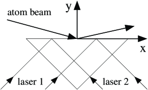
Figure 1: The geometry of the lasers and atomic beam in the evanescent field diffraction experiment. The atomic beam angles are exaggerated for clarity.

The modulus of the evanescent field wavevector $Q$ and its inverse decay length $q$ are [24]

$$Q=kn_{q}\sin\theta,\quad q=k\sqrt{(n_{q}\sin\theta)^{2}-1},$$ (1)

where $k$ is the free field wavevector modulus, assumed to be the same for each laser, $n_{q}$ is the refractive index of the quartz, and $\theta$ is the angle of incidence of the lasers with the quartz surface. The values of these parameters for the experiment we shall model are given in Table 1.

Table 1: Parameters used in experiment of Christ et al. [13].

Parameter	Value
Atom	Ne*
Atom mass	$3.3\times 10^{-26}$ kg
Atomic velocity	25 ms-1
Angle of incidence	36 mrad
Laser detunings	900 MHz
Transition wavelength	594.5 nm
$k$	$1.058\times 10^{7}$ m-1
$Q$	$1.10\times 10^{7}$ m-1
$q$	$2.72\times 10^{6}$ m-1

We assume that the atoms are initially in an eigenstate $|k_{0x}\rangle$ of the $x$-component of their momentum with eigenvalue $\hbar k_{0x}$. Then because the photon momentum of the copropagating (counterpropagating) field is $\hbar Q$ ($-\hbar Q$) the $x$-component of the atomic momentum is restricted to the eigenvalues $\hbar(k_{0x}+nQ)$, with $n$ any integer. We denote the corresponding set of allowed centre-of-mass $x$-momentum eigenstates by $\{|n\rangle,n\in\mathrm{integers}\}$. A ground (excited) state atom has $n$ even (odd).

The 3s[3/2]2 $\leftrightarrow$ 3p^′[3/2]2 transition of metastable neon is between states with total angular momentum J=2. Hence there are five ground $|m_{g}\rangle$, and five excited $|m_{e}\rangle$, sublevels labeled by the magnetic quantum numbers $m_{g/e}\in\{-2,-1,0,1,2\}$, Fig. 2.

Figure 2: Schematic diagram of the atomic level structure used in the model. The squares of the Clebsch-Gordon coefficients $C^{p}_{m_{g},m_{e}}$ for the transitions are shown.

The discrete basis states for the $x$-component of momentum and the internal state of the atom are therefore

$$|n,m\rangle\equiv|n\rangle\otimes|m\rangle.$$ (2)

Given our initial condition of ground state atoms the magnetic quantum number $m$ is $m_{g}$ ($m_{e}$) if $n$ is even (odd). The atomic motion in the $y$-direction, perpendicular to the quartz surface, is represented by one coordinate basis wavefunction $\Psi_{n,m}(y,t)$ for each discrete basis state $|n,m\rangle$. We use the following ansatz for the complete state of the atom

$$|\Psi(t)\rangle=\exp(-ik_{0x}^{2}t/2M\hbar)\sum_{m,n}\Psi_{n,m}(y,t)|n,m\rangle,$$ (3)

where $M$ is the atomic mass. The exponential prefactor accounts explicitly for the initial atomic kinetic energy in the $x$-direction.

The Hamiltonian $H$ for the system can be divided into two parts: the $y$-component of the kinetic energy $p_{y}^{2}/2M$, with continuous eigenvalues, and the rest $\{V+p_{x}^{2}/2M\}$, which has discrete eigenvalues,

$$H=\frac{p_{y}^{2}}{2M}+\left\{\frac{p_{x}^{2}}{2M}+V\right\}.$$ (4)

$p_{y}$ ($p_{x}$) is the $y$-component ($x$-component) of the atomic momentum perpendicular (parallel) to the quartz surface. $V$ is the sum of the atom’s internal energy and the electric dipole interaction energy between the evanescent field and the atomic transition $H_{\mathrm{ED}}$,

$$V=\sum_{m,n(\mathrm{odd})}\hbar\Delta_{a}|m,n\rangle\langle m,n|+H_{\mathrm{ED}},$$ (5)

This Hamiltonian is in an interaction picture with the atomic dipoles rotating at the average of the laser frequencies $\bar{\omega}=(\omega_{1}+\omega_{2})/2$, where $\omega_{1}(\omega_{2})$ is the frequency of the laser copropagating (counterpropagating) with the atoms. These frequencies can be different, as in the experiment of Stenlake et al. [12]. In that case they must be sufficiently similar that the approximation of equal photon momentum magnitudes holds. The atomic detuning $\Delta_{a}$ is the difference between the (degenerate) atomic transition frequencies and $\bar{\omega}$. The dipole interaction energy is

$$H_{\mathrm{ED}}=\mathbf{d}^{+}\cdot\mathbf{E}^{+}+\mathrm{H.c.}$$ (6)

where H.c. means Hermitean conjugate and $\mathbf{d}^{+}$ is the positive frequency part of the transition electric dipole moment operator $\mathbf{d}$

$$\mathbf{d}^{+}=\sum_{m_{g},m_{e}=-J}^{J}|m_{e}\rangle\langle m_{e}|{\bf d}|m_{g}\rangle\langle m_{g}|.$$ (7)

$\mathbf{E}^{+}$ is the positive frequency part of the total electric field

$$\mathbf{E}^{+}=\mbox{\boldmath$\varepsilon$}_{1}E_{1}(y,t)\exp(iQx)+\mbox{\boldmath$\varepsilon$}_{2}E_{2}(y,t)\exp(-iQx),$$ (8)

$$E_{i}(y,t)=\exp(-qy)\exp(-i\Delta_{d}t)E_{i0}.$$ (9)

$E_{10}$ ($E_{20}$) is the amplitude of the copropagating (counterpropagating) field at the quartz surface, and is assumed real for convenience. The $\mbox{\boldmath$\varepsilon$}_{i}$ are the corresponding field polarization vectors. $\Delta_{d}=(\omega_{1}-\omega_{2})/2$ is half the frequency difference between the two lasers. In the examples we consider in the next section $\Delta_{d}=0$.

We take the $z$ direction as the quantization axis and work with a spherical basis of polarization vectors $\{\mathbf{u}_{\pm},\mathbf{u}_{0}\}$ defined in terms of the Cartesian unit vectors by

$$\mathbf{u}_{\pm}=\frac{1}{\sqrt{2}}(\mathbf{u}_{x}\pm i\mathbf{u}_{y}),\quad\mathbf{u}_{0}=\mathbf{u}_{z}.$$ (10)

The Wigner-Eckart theorem [25] allows us to express the dipole matrix elements in terms of Clebsch-Gordon coefficients $C^{p}_{m_{g},m_{e}}$ and a reduced matrix element $\mathcal{D}$

$$\langle m_{e}|{\bf d}\cdot\mathbf{u}_{p}|m_{g}\rangle=C^{p}_{m_{g},m_{e}}\mathcal{D},$$ (11)

where $p$ is $0,\pm 1$ for $\pi,\sigma_{\pm}$ transitions. The values of the non-zero Clebsch-Gordon coefficients are indicated in Fig. 2. The dipole interaction Hamiltonian Eq. (6) then becomes

$$H_{\mathrm{ED}} = \mathcal{D}\sum_{p,m_{g},m_{e}}\left\{E_{1}(y,t)\sum_{n(even)}C^{p}_{m_{g},m_{e}}\varepsilon_{1,p}|m_{e},n+1\rangle\langle m_{g},n|\right.$$ (12)

$$\left.+E_{2}(y,t)\sum_{n(odd)}C^{p}_{m_{g},m_{e}}\varepsilon_{2,p}|m_{g},n+1\rangle\langle m_{e},n|\right\}+\mathrm{H.c.}$$

The $\varepsilon_{1/2,p}=\mbox{\boldmath$\varepsilon$}_{1/2}\cdot\mathbf{u}_{p}$ are the spherical polarization components of the two lasers.

Substituting the ansatz Eq. (3) into the Schrödinger equation corresponding to the Hamiltonian Eq. (4) gives the set of coupled Schrödinger equations

$$i\partial_{t}\Psi_{n,m_{e/g}} = \left[\frac{p_{y}^{2}}{2M\hbar}+S_{n}\right]\Psi_{n,m_{e/g}}$$ (13)

$$+\sum_{n^{\prime},m_{e/g}^{\prime}}\langle n,m_{e/g}|V|n^{\prime},m_{e/g}^{\prime}\rangle\Psi_{n^{\prime},m_{e/g}^{\prime}}\quad,$$

$$S_{n}\equiv\frac{\hbar}{2M}(2k_{0,x}nQ+n^{2}Q^{2}).$$ (14)

We have solved this set of partial differential equations numerically by the well known split operator method [19]. Our numerical solutions were checked for accuracy by demanding that changing either the time-step or the spatial grid size did not significantly alter the final result.

3 Diffraction

Before presenting numerical solutions of the Schrödinger equations we consider the quasipotentials of the Hamiltonian Eq. (4) [17]. These are the eigenvalues of that part of the Hamiltonian having discrete eigenvalues, namely $\{V+p_{x}^{2}/2M\}$ Eq. (5). Since $V$ includes the interaction with the evanescent field the quasipotentials are a function of $y$, the distance from the quartz surface. The eigenstates corresponding to the quasipotentials may be thought of as atomic states doubly dressed by the two evanescent fields.

The eigenstates of $V$ corresponding to the quasipotentials are adiabatically followed by atoms moving sufficiently slowly towards the surface, except near avoided crossings of the quasipotentials. Hence they behave like actual potentials, for example slowing atoms down as they climb them, which is the origin of atomic reflection [26]. At the avoided crossings non-adiabatic transitions between the quasipotentials may occur. These make diffraction possible, since the atoms may leave the evanescent field in a different superposition of quasipotential eigenstates than that in which they entered, and different eigenstates may have different momenta.

A two-level atom model allows diffraction for certain ranges of parameters. In particular the diffraction considered by Deutschmann et al. [17] occurred for much lower atomic detunings than were used in the experiment of Christ et al. [13]. The lower detunings would have produced unacceptable levels of atomic excitation and hence of spontaneous emission.

Since excited states spontaneously emit, diffraction into ground states, with even $n$, is of most interest. The optimum probability for the $n=\pm 2$ diffraction orders was estimated to be about 6% by Deutschmann et al. [17]. This is because at least four avoided crossings are required, with an optimal transfer probability of 50% at each, and $0.5^{4}\approx 0.06$. The quasipotentials for a two-level model of the experiment are shown in Fig. 3(a). Note that the incoming $n=0$ quasipotential only has avoided crossings with high order quasipotentials, the first being with the $n=21$ quasipotential [20]. The transition between the corresponding eigenstates would involve a 21 photon process and hence be very weak, giving negligible $n=-2$ order diffraction. This is inconsistent with the observations of Christ et al. [13].

Figure 3: Quasipotentials versus perpendicular distance from the quartz surface, for the parameters of Table 1. (a) Two-level quasipotentials. (b) Multi-level quasipotentials for a laser polarization angle of $5^{\circ}$ away from p-polarization.

The quasipotentials for the multi-level atom model of the experiment are shown in Fig. 3(b). The multi-level model makes possible Raman transitions between the ground Zeeman levels. Hence there is now an avoided crossing between $n=0$ and $n=-2$ quasipotentials, so diffraction into an $n=-2$ eigenstate is expected.

The experiment of Christ et al. [13] that we have modelled reported up to 3% diffraction. The ratio of the intensities of the copropagating to counterpropagating waves was fixed at 1.64. To calculate the diffracted fraction we numerically solved the Schrödinger equations (13), as described in the previous section. Our results are quite sensitive to the polarizations of the two laser beams [21]. Fig. 4 shows the percentage of diffraction into the $n=-2$ order as a function of the polarization angle of the lasers. The results in this figure were calculated for an equal mixture of magnetic sublevels in the incoming atomic beam.

We did not calculate the diffraction from all initial $m_{g}$ states for all polarization angles. This was because each point on Fig. 4 took approximately 30 minutes to compute on a VPP300 supercomputer. Typically the spatial grid in the $y$ direction had 2048 elements and 13 $n$ states, $n=-6$ to $n=6$ were used. The integration over 1.6 $\mu$s was performed with 0.2 ns timesteps. These numerical parameters were varied to ensure the insensitivity of the solutions.

However we did calculate for all $m_{g}$ states for several representative polarisation angles, and in all cases it was found that they produced amounts of diffraction bearing a fixed ratio to each other. This is because only one of the $n=0$ quasipotentials is involved in the diffraction process, and the various $m_{g}$ states enter this quasipotential in fixed ratios. This observation allowed us to deduce the overall diffraction for a mixture of magnetic sublevels.

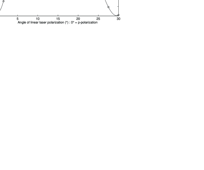
Figure 4: Percentage $n=-2$ order diffraction versus polarization angle for an incoming $m_{g}=2$ atom. The percentage of diffraction is plotted versus the linear polarization angle, in degrees, of the two laser beams from pure p-polarization, $0^{\circ}$. The solid curve is a fit to the calculated points. Other parameters are as in Table 1.

We have also modelled the conditions which gave maximum diffraction according to unpublished experimental data [20]: The polarization of the copropagating beam rotated by 5 degrees from perfect p-polarization (electric field in the plane of incidence) and the counterpropagating beam rotated 15 degrees from perfect p-polarization [20]. Despite uncertainty as to the accuracy of these figures, we found that these parameters gave a large degree of diffraction (about 14%). Furthermore, a ratio of 1.64 between the co-propagating and counterpropagating beams was cited as an important condition for diffraction to occur [13]. Computationally, we found that this condition produced a local maximum in the amount of diffraction.

These results demonstrate that a multi-level model is able to account for the diffraction observed by Christ et al. [13]. The difference between the diffraction we find (14% for experimental parameters) and that observed, 3%, is reasonable given the non-ideal aspects of the experiment and the lack of delicate control over the parameters.

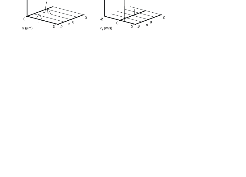
Figure 5: Probability densities in position and momentum spaces for an initial $m_{g}=2$ state atom. The probability density $P_{n}=\sum_{m}|\Psi_{n,m}|^{2}$ is plotted against the diffraction order $n$ and either the distance from the glass in microns (a) and (b), or the velocity perpendicular to the glass (c) and (d). In each case the top figure is the initial condition and the bottom figure is 1.6 $\mu$s later, after reflection. There is no probability in the orders not shown. Parameters are as in Table 1 with laser polarizations of $5^{\circ}$ away from p-polarization.

One of the advantages of numerically solving the time-dependent Schrödinger equation is that “movies” of the wavefunction evolution are available. The wavefunction can be visualized in either coordinate or momentum space. Fig. 5 shows an initial $m_{g}=2,n=0$ probability density evolving to produce $n=-2$ order diffraction.

4 Conclusion

We have quantitatively modeled, from first principles, the reflection grating atomic diffraction experiment of Christ et al. [13]. Our results are consistent with the levels of diffraction observed in that experiment. The model predicts strong dependence on the polarization of the copropagating and counterpropagating laser beams. This is physically reasonable since the atomic Zeeman structure makes the shifts of the various atomic transitions polarization dependent. There is some evidence for this effect in the experiment [20].

Computational modelling of experiments, such as we have reported, is particularly useful if it can suggest new experiments. Our results show that control of the polarization of both laser beams is crucial in reflection grating atomic diffraction experiments. Furthermore we found that under the conditions of the experiment of Christ et al. [13] the Zeeman $m_{g}=2$ state produced most of the $n=-2$ order diffraction. Hence optical pumping into this state could potentially increase the diffraction.

Our model is easily adapted to other atoms and we plan to use it to model a Caesium evanescent wave diffraction experiment currently underway in our group.

References

- [1] C. S. Adams, M. Sigel and J. Mlynek, Phys. Rep. 240 (1994) 1.
- [2] C. S. Adams, O. Carnal and J. Mlynek, Adv. Atomic Mol. Opt. Phys. 34 (1994) 1.
- [3] E.M. Rasel, M.K. Oberthaler, H. Batelaan, J. Schiedmayer, and A. Zeilinger, Phys. Rev. Lett 75, 2633 (1995).
- [4] D.M. Giltner, R.W. McGowan, S.A. Lee, Phys. Rev. Lett 75, 2638 (1995).
- [5] V.I. Balykin, V.S. Letokhov, Yu.B. Ovchinnikov, and A.I. Sidorov, Phys. Rev. Lett 60, 2137 (1988).
- [6] J.V. Hajnal, K.G.H. Baldwin, P.T.H. Fisk, H.-A. Bachor, and G.I. Opat, Optics Comm. 73, 331 (1989).
- [7] M.A. Kasevich, D.S. Weiss, and S. Chu, Optics Lett. 15, 607 (1990).
- [8] C.G. Aminoff, A.M. Steane, P. Bouyer, P. Desbiolles, J. Dalibard, and C. Cohen-Tannoudji, Phys. Rev. Lett 71, 3083 (1993).
- [9] W. Seifert, C.S. Adams, V.I. Balykin, C. Heine, Yu. Ovchinnikov, and J. Mlynek, Phys. Rev. A 49, 3814 (1994).
- [10] W. Seifert, R. Kaiser, A. Aspect, and J. Mlynek, Optics Comm. 111, 566 (1994).
- [11] S. Feron, J. Reinhardt, M. Ducloy, O. Gorceix, S. Nic Chormaic, Ch. Miniatura, J. Robert, J. Baudon, V. Lorent, and H. Haberland, Phys. Rev. A 49, 4733 (1994).
- [12] B. W. Stenlake, I.C.M. Littler, H.-A. Bachor, K.G.H. Baldwin, and P.T.H. Fisk, Phys. Rev. A 49, 16 (1994).
- [13] M. Christ, A. Scholz, M. Schiffer, R. Deutschmann, and W. Ertmer, Optics Comm. 107 (1994) 211.
- [14] R. Brouri, R. Asimov, M. Gorlicki, S. Feron, J. Reinhardt, and V. Lorent, preprint (1996).
- [15] J.V. Hajnal and G.I. Opat, Optics Comm. 71 (1989) 119.
- [16] R.J. Cook and R.K. Hill, Optics Comm. 43 (1982) 258.
- [17] R. Deutschmann, W. Ertmer, and H. Wallis, Phys. Rev. A 47 (1993) 2169.
- [18] J.E. Murphy, L. Hollenberg , and A.E. Smith, Phys. Rev. A 49 (1994) 3100.
- [19] C. Savage, D. Gordon, and T. Ralph, Phys. Rev. A 52 (1995) 4741.
- [20] R. Deutschmann and M. Schiffer, personal communications (1995, 1996).
- [21] R. Deutschmann, W. Ertmer, and H. Wallis, Phys. Rev. A 48 (1993) R4023.
- [22] G. Orriols, Nuovo Cimento 53B (1979) 1.
- [23] S. Tan and D. Walls, Phys. Rev. A 50 (1994) 1561.
- [24] M. Born and E. Wolf, Principles of Optics (Wiley, NY, 1980).
- [25] E. Merzbacher, Quantum Mechanics (Pergamon, Oxford, 1970).
- [26] C. Savage, Aust. J. Physics 49, (1996) 745.