Cosmic Star Formation Rate from Gamma-Ray Attenuation

Abstract

We compute the attenuation of gamma-rays from remote quasars due to interactions with ambient low-energy photons produced by stars in galaxies and show that the next-generation gamma ray telescopes can probe the cosmic star formation rate at high redshifts.

1 Introduction

The cosmic star formation rate (CSFR) at high redshifts is a key probe to determine the time-table of structure formation in the universe and hence to further constrain cosmology. Number counts of galaxies only give access to small parts of the sky and are subject to severe selection effects depending on the wavelength range of the observational campaign such as, for example, extinction by dust using deep photometry in the optical. Furthermore, absolute sky photometry is biased due to galactic foregrounds making it difficult to assess truly diffuse extragalactic background light (EBL) which could arise due to the decay of unstable relics from the early universe. Therefore, an independent method unaffected by these obstacles is required, and we suggest along with Salamon & Stecker (1998) and Primack et al. (1999) to use the attenuation of gamma rays from distant quasars for this purpose.

EGRET has detected that many flat-spectrum radio quasars at high redshifts emit gamma rays at least up to 10 GeV showing generally no indication for a spectral break. A few nearby flat-spectrum radio sources have even been detected up to TeV ($10^{12}$ eV) energies using ground-based Cherenkov telescopes suggesting that at least some of the sources exhibit smooth power-law spectra in the GeV-to-TeV energy range. The gamma rays of energy $E_{\gamma}$ can interact with ambient low-energy photons of energy $\epsilon$ creating electron-positron pairs provided the threshold energy $E_{\gamma}\sim(m_{e}c^{2})^{2}/\epsilon$ is exceeded. As a result, the gamma ray sources should show a cutoff in their spectrum at the energy where the mean free path for pair creation becomes shorter than the distance to the sources, i.e. where $\tau_{\gamma\gamma}(E_{\gamma})\sim\sigma_{\gamma\gamma}n_{\rm ebl}[(m_{e}c^{2})^{2}/E_{\gamma}]d_{z}\geq 1$ where $\sigma_{\gamma\gamma}\simeq\sigma_{\rm T}/3$, $n_{\rm ebl}$ denotes the photon number density of the EBL, and $d_{z}$ is the cosmological distance of the gamma ray source. Generally, since the number density of background photons increases with decreasing photon energy, and thus increasing gamma ray energy above threshold, the more distant gamma ray sources must show lower cutoff energies than the closer gamma ray sources and the precise running of the cutoff energies with redshift will tell us about the shape and evolution of the EBL.

Our strategy now is to develop a simple model for the redshift-dependent EBL based on the observed (and extinction-corrected) CSFR and then to determine the corresponding values of gamma ray cutoff energies. We start with a description of the galaxy evolution templates used to determine the EBL when folded with the CSFR, and proceed with the computation of the gamma ray optical depth. Finally, we discuss that possible deviations of future measurements of the gamma ray cutoff energies would require changes in the EBL model (e.g. in the CSFR) or force us to consider additional sources to contribute to the EBL.

2 Spectral energy distribution

Figure 1: Spectral energy distribution of a simple stellar population with mass $10^{11}M_{\odot}$ and solar metalicity evolving from an age of 0.01 Gyrs to 17 Gyrs.

We use the spectral synthesis model calculated by Möller et al. (1999), which describes the evolution of the spectral energy distribution (SED) of a single burst population (SSP) with time (see Figure 1). The stars have solar metalicity and Salpeter IMF. We simplify the temporal evolution by reducing it to only two spectral states. The first state lasts from ignition to an age of 0.28 Gyrs. We call this state the early phase and it is dominated by the ultraviolet and optical radiation of young massive stars. The second state is defined to begin at an age of 0.28 Gyrs. We call this state the late phase and it is dominated by the optical and infrared light of the older stars in the population. To get the spectrum representative for each phase we calculate the corresponding mean SED from the templates. Note that the late phase lasts over a cosmologically significant portion of time and therefore must be weighted with the CSFR. Furthermore, we include the effect of the interstellar medium (ISM) by assuming an isotropic and homogeneous gas and dust distribution around the stars of the SSP. We use Osterbrook’s Case B for optical thick gas clouds, i.e. total absorbtion of photons below the wavelength of 911 Å and reemission of the absorbed power in the optical regime by bremsstrahlung and $H_{\alpha}$ line emission. The dust is treated the same way as in Desert et al. (1990) considering a three component model with big grains, small grains and PAH’s. For the absorbtion we use an extinction curve similar to the one of the SMC. The reemission is described by four Planck spectra with two temperatures for each phase reprensenting warm and cold dust components. The resulting spectra including absorbtion and re-emission are shown in figure 2.

Figure 2: Spectral energy distributions of a simple stellar population for the early (the first 0.28 Gyrs) and late (after 0.28 Gyrs) phases. The solid line includes (dashed line excludes) absorbtion and reemission of the ISM.

3 Cosmic star formation rate

Now let us look at galaxy evolution on global scales. In our model, the stars in galaxies are all represented by SSPs. So far we did not include a particular star formation rate, and we will do this now by using the cosmic star formation rate (CSFR) as determined from galaxy counts in the optical (e.g., Madau 1996). Since dust and gas absorbs optical photons, the original Madau CSFR underestimates the true SFR in particular at high redshifts by at least a factor of $\sim 3$ (Pettini et al. 1998) or maybe even $\sim 4.7$ (Steidel et al. 1999). All data agree, however, in a CSFR increasing up to a redshift $z=z_{\rm b}\sim 1-2$ and decreasing at $z>z_{\rm b}$, see Fig. 3. We adopt in the following a power-law fit to this CSFR shown as the solid line in Fig. 3

$$\dot{\rho_{\ast}}(z)\propto(1+z)^{\alpha}$$ (1)

with $\alpha=\alpha_{m}>0$ for $z<z_{b}$ and $\alpha=\beta_{m}<0$ for $z>z_{b}$.

Figure 3: Cosmic star formation rate $\stackrel{{\scriptstyle\cdot}}{{\rho}}_{\ast}$ vs. redshift $z$. The data are taken from Madau (1996; solid circles), corrected by Pettini et al. (1998; open squares), Gallego (1995; diamond) and further data from Steidel et al. (1999; stars). The solid line indicates the fit used in our model

4 Emissivity

Solving the convolution integral

$$\mathcal{E}_{\lambda}(t)=\int_{0}^{t}\mathcal{F}_{\lambda}(t-t^{\prime})\stackrel{{\scriptstyle\cdot}}{{\rho_{\ast}}}(t^{\prime})dt^{\prime}$$

we can calculate the emissivity at different cosmic times $t=t(z)$. For the comparison with measurments we will integrate over redshift $z$ and change to the comoving emissivity

$$\mathcal{E}_{\lambda}(z)=(1+z)^{-2}\int_{z}^{z_{m}}\mathcal{F}_{\lambda}(t(z)-t(z^{\prime}))\stackrel{{\scriptstyle\cdot}}{{\rho}}_{\ast}(z^{\prime})\frac{dt^{\prime}}{dz^{\prime}}dz^{\prime}.$$ (2)

We used the parameters in Tab. 1 to obtain the results shown in Fig. 4. The emissivity $\mathcal{E}_{\lambda}(z)$ is plotted for three different wavelengths demonstrating satisfactory agreement. Note that in particular the steeper increase at 0.28 $\mu$m and the more shallow increase at 1.0 $\mu$m are well reproduced by the model.

$E_{B-V}^{e}$	$E_{B-V}^{l}$	$\alpha_{m}$	$\beta_{m}$	$z_{b}$	$y_{m}[M_{\odot}yr^{-1}Mpc^{-3}]$
0.1	0.03	3.4	-2	1.3	0.13

Table 1: Choosen parameter for the calculation of the emissivity. Note that we used the better value $\beta_{m}=-1$ for the CSFR (Fig. 3) and the background (Fig. 5) calculation.

Figure 4: Emissivity vs. redshift . Data taken from Lilly et al. (1996; squares), Conolly et al. (1997; circles) and Ellis et al. (1996; dots).

5 Extragalactic background light

The intensity of the EBL follows from the emissivity

$$\lambda I_{\lambda}=\lambda\frac{c}{4\pi}\int_{z}^{z_{m}}\mathcal{E}_{\lambda^{\prime}}(z)\frac{dt^{\prime}}{dz^{\prime}}\left(\frac{1+z}{1+z^{\prime}}\right)^{2}dz^{\prime}.$$ (3)

We compute the background intensity at several redshifts and show the results in Fig. 5. Beyond a redshift of $z\sim 1.3$, the EBL decreases because of the decreasing CSFR and the expansion of the universe. The shape of the spectrum at high redshifts is determined by the early phase spectrum, whereas for lower redshifts the late phase becomes more and more important. This is a consequence of of the maximum star formation rate at redshifts $z=1-2$ from which the stellar populations have considerably aged until the present. There are no direct measurements of the EBL at high redshift (with the exception of inferences of the UV background based on the proximity effect which are consistent with our model predictions if we employ empirical power law extensions of the UV spectra beyond the Lyman edge). We can, however, compare our results with the present-day data obtaining good agreement as shown in Fig. 6.

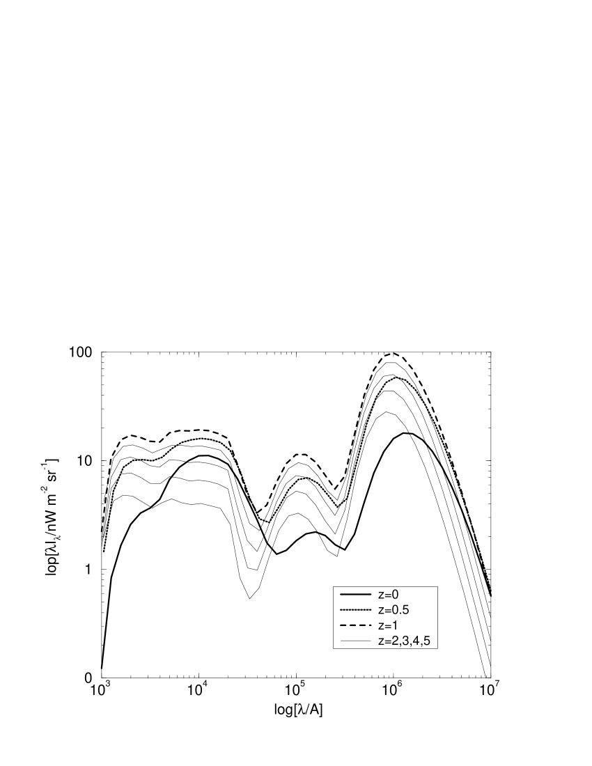
Figure 5: Diffuse Extragalactic background light due to stars in galaxies, for various redshifts.

6 Gamma ray attenuation

The gamma-ray attenuation can be parametrized by the optical depth for photon-photon pair production

$$\tau(E_{\gamma},z_{q})=c\int_{0}^{z_{q}}\int_{0}^{2}\int_{\epsilon_{gr}}^{\infty}\frac{dl}{dz^{\prime}}\frac{\mu}{2}n_{\rm ebl}(\epsilon,z^{\prime})(1+z)^{3}\cdot$$ (4)

$$\cdot\sigma_{\gamma\gamma}(E_{\gamma},\epsilon,\mu,z^{\prime})d\epsilon\ d\mu\ dz^{\prime}$$

Using Eq. (3) for the intensity of the background photons we can calculate the number density $n_{\rm ebl}(\epsilon,z^{\prime})$. Inserting $n_{\rm ebl}(\epsilon,z^{\prime})$ in Eq. (4) we can compute the optical depth for various redshifts. The optical depth enters the attenuation factor $\exp[-\tau(E_{\gamma},z_{q})]$ for gamma rays (see Fig. 7) modifying quasar power law spectra. Future gamma ray observations with ground-based air Cherenkov telescopes in the energy range 10 GeV to 10 TeV can efficiently probe the run of the CSFR with redshift. E.g., the faster the decrease above the maximum of the CSFR (the larger the slope $\beta_{m}$ in Eq. (1)), the less attenuation occurs for quasars at redshifts $z\gg 1$. On the other hand, a plateauish CSFR combined with the effect of dust keeps the UV radiation density low at high redshifts, but leads to a strong FIR bump in the EBL which leads to strong attenuation of $>$ 10 TeV gamma rays from nearby $z\ll 1$ radio sources.

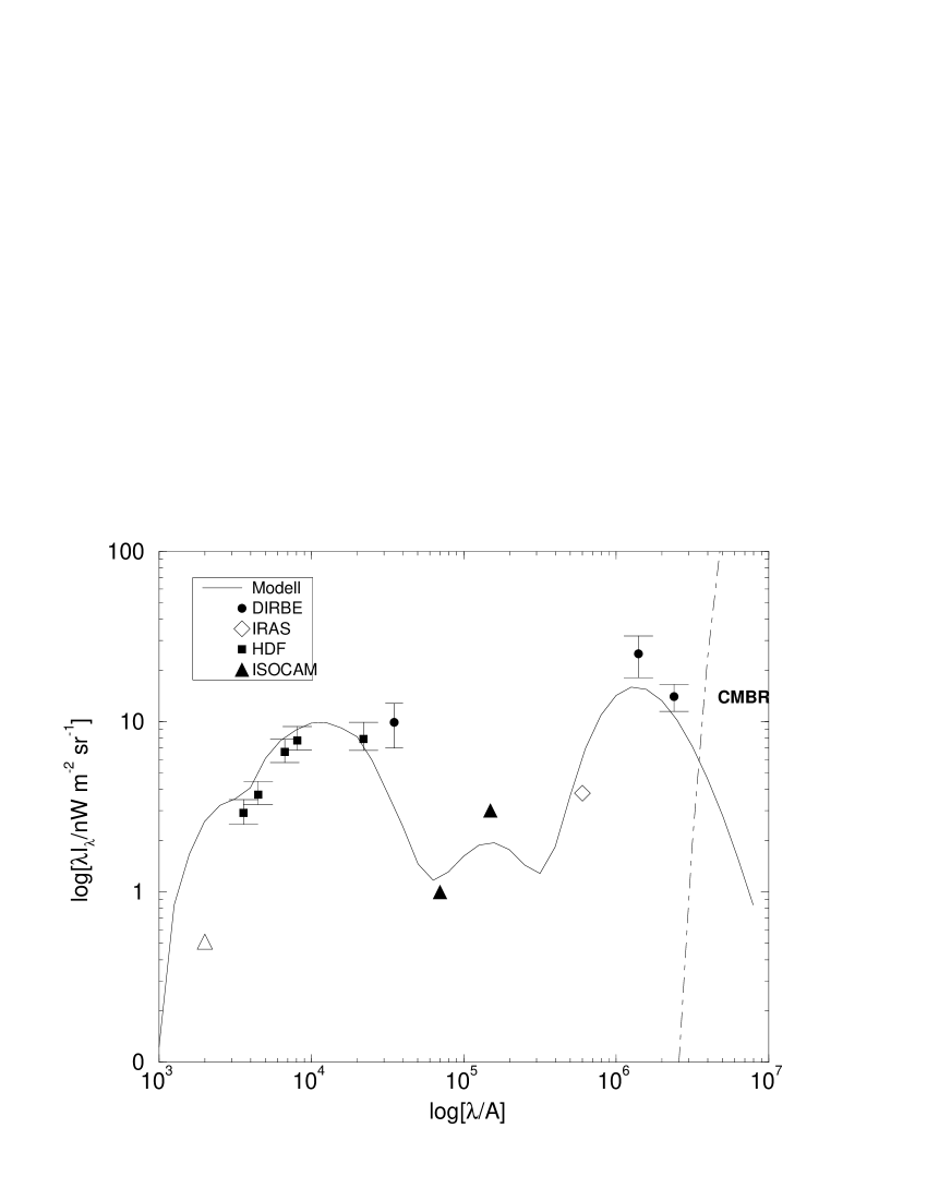
Figure 6: Comparison of the model with the observed present-day EBL. Data points refer to Armand et al. (1994; open triangle), Pozetti et al. (1998; squares/HST), Dwek et al. (1998; filled circle at 35$\mu$m/DIRBE), Altieri et al. (1998; triangle/ISOCAM), and Hauser et al. (1998; diamond/IRAS, blue filled circles/DIRBE).

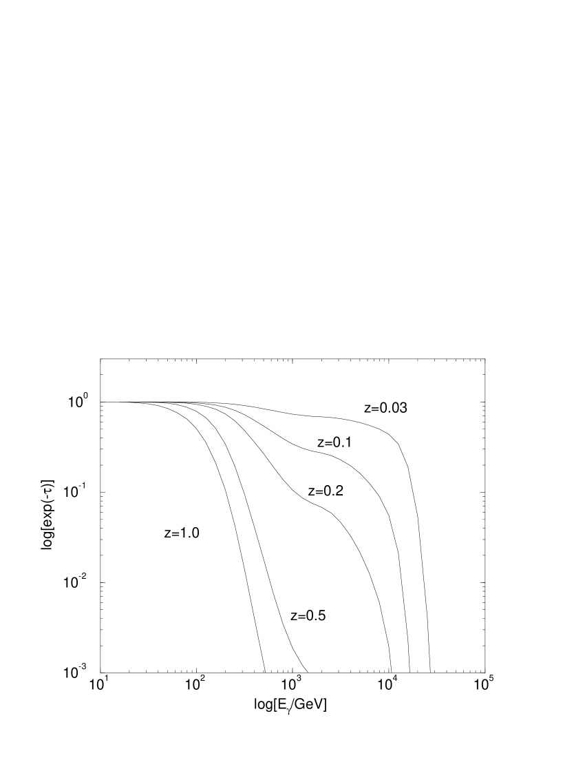
Figure 7: Attenuation factor $\exp[-\tau(E_{\gamma},z_{q})]$ for gamma-rays as a function of gamma ray energy $E_{\gamma}$ for various quasar redshifts $z_{q}$.

7 Summary and conclusions

In order to facilitate a comparison of gamma ray cutoff energies in the spectra of high-redshift quasars with theoretical predictions of gamma ray attenuation due to pair creation, we developed a simple model for the evolving EBL based on the observed CSFR taking into account extinction and re-emission by dust and gas. Further model inputs are the IMF, the average metalicity, relative contributions of warm and cold dust to the emission of early- and late-type galaxies, and the Hubble constant for which we have adopted values in close agreement with observations. The CSFR at high redshifts is not accurately determined by the data, and we have tried to use a value which is consistent with both the present-day EBL and high-redshift galaxy counts. So far we have neither considered the extension of the galaxy spectra beyond the Lyman edge, the metalicity dependence of galaxy spectra, nor the contribution of quasars to the EBL. The predicted attenuation of gamma rays from nearby radio sources such as Mrk501 or Mrk421 leads to a quasi-exponential cutoff near 10 TeV due to interactions with the infrared part of the EBL, and to a cutoff near 100 GeV due to interactions with the optical/UV part of the EBL for sources with redshifts in excess of one.

References

- [] Altieri, B. 1998, A&A 343, 65
- [] Armand, C. 1994 A&A 284, 12
- [] Conolly, A.J. et al. 1997 ApJ 486, L11
- [] Dwek, E., Arendt, R.G. 1998 ApJ 508
- [] Ellis, R. S., Colless, M., Broadhurst, T., Heye, J., Glazerbrook, K. 1996 MNRAS 280, 235
- [] Gallego, J., Zamorano, J., Aragon-Salamanca, A., Rego, M.1995 ApJ 455, L1
- [] Hauser, M.G. et al. 1998 ApJ 508, 25
- [] Kneiske, T.M., Mannheim, K. 2000 in prep.
- [] Lilly, S.J. et al. 1996 ApJ 460, L1
- [] Madau,P.(1996) astro-ph/9612157
- [] Möller, C.S., Fritze-v.Alvesleben U., Fricke, K.J. 1999 in prep.
- [] Pettini, M, Steidel, C.C., Adelberger, K.L., Kellog, M., Dickinson, M., Giavalisco, M. 1998 ASP Conference Sereies 148, 67
- [] Primack, J.R., Bullock, J.S., Somerville, R.S., MacMinn, D. 1999 APh 11, 93
- [] Salamon, M.H., Stecker, F.W. 1998, ApJ 439, 547
- [] Steidel, C.C., Adelberger, K.L., Giavalisco, M., Dickinson, M., Pettini, M. 1999 ApJ 519, 1