New Improved Photometric Redshifts of Galaxies in the HDF

Abstract

We report new improved photometric redshifts of 1048 galaxies in the Hubble Deep Field (HDF). A standard $\chi^{2}$ minimizing method is applied to seven-color UBVIJHK photometry by Fernández-Soto, Lanzetta, & Yahil (1999). We use 187 template SEDs representing a wide variety of morphology and age of observed galaxies based on a population synthesis model by Kodama & Arimoto (1997). We introduce two new recipes. First, the amount of the internal absorption is changed as a free parameter in the range of $E(B-V)=0.0$ to $0.5$ with an interval of $0.1$. Second, the absorption due to intergalactic HI clouds is also changed by a factor of 0.5, 1.0, and 1.5 around the opacity given by Madau (1995). The total number of template SEDs is thus $187\times 6\times 3=3,366$, except for the redshift grid. The dispersion $\sigma_{z}$ of our photometric redshifts with respect to spectroscopic redshifts is $\sigma_{z}=0.08$ and $0.24$ for $z<2$ and $z>2$, respectively, which are smaller than the corresponding values ($\sigma_{z}=0.09$ and $0.45$) by Fernández-Soto et al. Improvement is significant, especially in $z>2$. This is due to smaller systematic errors which are largely reduced mainly by including three opacities due to intergalactic HI clouds. We discuss redshift distribution $N(z)$ and cosmic star formation rate based on our new photometric redshifts.

1. INTRODUCTION

Large redshift surveys of galaxies have played a quite important role for understanding the formation and evolution of galaxies. In 1990’s, several new deep redshift surveys using large optical telescopes were carried out: e.g., Canada-France Redshift Survey (CFRS; Lilly et al. 1995), Hawaii Deep Field (Cowie et al. 1996), Autofib/LDSS survey (Ellis et al. 1996), the Canadian Network for Observational Cosmology (CNOC1,2 surveys; Yee et al. 1996 and Carlberg et al. 1998). Some of those surveys reach as deep as $z\sim 1$, and we have obtained some information about the formation and evolution of galaxies up to $z\sim 1$. However, little has been known about the properties of $z>1$ galaxies from such redshift surveys due to the limited depth of spectroscopic observations. Even if one uses LRIS with a Keck telescope, the limiting magnitude of spectroscopy is about R${}_{\rm lim}\simeq 25$, while the limiting magnitude of photometry with Hubble Space Telescope (HST) WFPC2 is $R_{\rm lim}\simeq 28-29$.

There is, however, so called ‘photometric redshift technique’, which enables us to measure redshifts of faint galaxies. Photometric redshift technique was originally suggested by Baum et al. (1963) to determine redshifts of some clusters of galaxies based on multi-band photometry using mean spectra of their member galaxies. There were, however, only a few applications of the technique (e.g., Koo 1985; Loh & Spillar 1986) before it revived recently to study distant galaxies, in particular, faint galaxies found in the Hubble Deep Field (HDF; Williams et al. 1996) (Connolly et al. 1995; Lanzetta, Yahil, & Fernández-Soto 1996, 1998; Gwyn & Hartwick 1996; Mobasher et al. 1996; Sawicki, Lin, & Yee 1997; Connolly et al. 1997). Photometric redshift technique is the only method available at present to infer the redshifts of galaxies beyond the spectroscopic limit.

In this work we improve the accuracy of photometric redshifts of galaxies in the HDF by using a set of template spectral energy distribution (SED). We treat the internal absorption of galaxies and the extinction due to intergalactic HI clouds more carefully than previous studies. We adopt a technique based on a standard $\chi^{2}$ minimizing method with a template set which consists of simulated SEDs. We apply it to a photometry catalog of galaxies in the HDF (Fernández-Soto, Lanzetta, & Yahil 1999), which is the deepest catalog available with some spectroscopic redshifts.

The detailed method, adopted parameters of simulated SEDs, and the comparison between our photometric redshifts and spectroscopic redshifts are described in § 2. We show in § 3 the comparison of our improved photometric redshifts with previous studies and the validity of our result. We present our improved photometric redshift for the HDF galaxies in § 4, where we also discuss the properties of the HDF galaxies such as redshift distribution and cosmic star formation rate. Conclusions are given in § 5.

2. METHOD

We may classify photometric redshift techniques into two categories. One is the training-set method (Connolly et al. 1997, Wang et al. 1999) and the other is the $\chi^{2}$ minimizing method (Gwyn & Hartwick 1996; ; Mobasher et al. 1996, 1999; Sawicki et al. 1997; Giallongo et al. 1998).

The training-set method first makes an empirical formula by fitting polynominals to the photometry data of galaxies with known redshifts. It then applies the same formula to photometry data of new galaxy samples to determine their photometric redshifts. This method is superior to the other in the point that the more galaxies we observe for the training set, the more accurate photometric redshifts we obtain. Therefore, Yee (1998) called it the empirical training-set method. For low-z galaxies, the training-set method seems to work more robust than the $\chi^{2}$ method, because it is based on real observed galaxy spectra and because the empirical formula can be determined accurately using a large number of spectroscopic samples (Connolly et al. 1997). Recently, comparably accurate redshifts are obtained by a simpler training-set method which adopts binning of galaxies according to observed colors (Wang, Bahcall & Turner 1998; Wang, Turner, & Bahcall 1999). Csabai, Connolly, & Szalay (1999) also succeeded in obtaining accurate photometric redshifts by combining the training-set method and the $\chi^{2}$ method. However, it is difficult to make a good training set for high redshift galaxies, since the number of galaxies with spectroscopic redshifts is still small. Also we should be cautious in applying the empirical formula obtained at low redshifts to high redshift galaxies, since significant evolution is expected in their SEDs.

Hence, in this study, we use the $\chi^{2}$ minimizing method which can include spectral evolution of galaxies directly. This method searches for the best-fit SED and the redshift of a galaxy by comparing the observed SED of the galaxy with templates prepared in advance. In general, templates are made either from observed spectra of nearby galaxies or from simulated spectra based on a population synthesis model. Coleman, Wu, & Weedman (1980; hereafter CWW) and Kinney et al. (1993, 1996) are widely used sources of observed spectra for the HDF galaxies. Lanzetta et al. (1996, 1998) and Fernández-Soto et al. (1999) used CWW’s and Kinney et al.’s spectra. However, the use of the observed SEDs of nearby galaxies may make it difficult to directly take the effects of galaxy evolution into account. Accordingly, in this paper we use simulated spectra based on a recent population synthesis model. Gwyn & Hartwick (1996) also used simulated spectra based on Bruzual & Charlot (1993). Sawicki et al. (1997) made their templates based on both observed spectra (CWW) and simulated spectra by Bruzual & Charlot (1996; hereafter BC96).

2.1. Template SEDs

We use a stellar population synthesis model by Kodama & Arimoto (1997; hereafter KA97) to make template SEDs. KA97 includes the stellar evolutionary tracks after the asymptotic giant branch in addition to the conventional tracks. Hence the model predicts UV flux of galaxies reasonably well, or at least, as good as any previous models. KA97 was successfully used to obtain photometric redshifts of low redshift galaxies (Kodama, Bell, & Bower 1999). Our work is the first to use KA97 to obtain photometric redshifts of high-$z$ galaxies.

The template SEDs consist of the spectra of pure disks, pure bulges, and composites made by interpolating the two as shown in Table 1. The parameters for the SEDs are the power-law index $x^{\rm IMF}$ of the initial mass function (IMF), the time scale of star formation $\tau_{\rm SF}$, the time scale of gas infall from a galactic halo into a disk $\tau_{\rm infall}$, and the time when the galactic wind blows $t_{\rm GW}$. The star formation rate of a galaxy is set to be zero after $t_{\rm GW}$. For disks, we adopt $x^{\rm IMF}=1.35$, $\tau_{\rm SF}=5$Gyr, $\tau_{\rm infall}=5$Gyr, and $t_{\rm GW}=20$Gyr (i.e., longer than the present age of the universe), which are close to the values estimated for the disk of our Galaxy. We adopt from KA97 $x^{\rm IMF}=1.10$, $\tau_{\rm SF}=0.1$Gyr, $\tau_{\rm infall}=0.1$Gyr, and $t_{\rm GW}=0.353$Gyr for bulges, which are known to reproduce the average color of ellipticals in clusters of galaxies. We make intermediate SED types by combining a disk component and a bulge component with the same age. The ratio of the bulge luminosity to the total luminosity in the B band, which we define as B/T, is changed from 0.1 to 0.9 with an interval of 0.1. Pure disk SEDs correspond to young or active star-forming galaxies, and pure bulge SEDs correspond to elliptical galaxies. We also prepare very blue SEDs of age$<$1Gyr, corresponding to blue star-forming galaxies reported by recent deep surveys. In total, our basic template set consists of 187 SEDs.

2.2. The Absorption Effects

To simulate the observed SEDs, we take into account two absorption effects. One is the internal absorption due to dust in each galaxy. More light is scattered and absorbed by dust grains in shorter wavelengths. Therefore, internal absorption is one of the key parameters for photometric redshift technique which is sensitive to wavelength dependent effects. For simplicity, we assume that all galaxies have the same extinction curve, although we change the absolute amount of extinction, indicated by $E(B-V)$, as a free parameter.

Typical features of extinction curves of nearby galaxies including our Galaxy are as follows: (1) The amount of absorption basically increases from the infra-red to the ultraviolet. (2) Some extinction curves have a bump at 2175Å, which is usually explained mainly by graphite. The existence of the bump is reported for our Galaxy (Seaton 1979; Cardelli et al. 1989), LMC (Fitzpatrick 1985), and M31 (Bianchi et al. 1996). However, no bump is reported in the extinction curve of SMC (Prévot et al. 1984; Bouchet et al. 1985). Gordon, Calzetti, & Witt (1997) showed that whether the bump is present or not cannot be explained by scattering or geometrical effects, and that galaxies with high star formation activity tend to have no bump in their extinction curves.

There are some studies in which an analytical formula was fitted to observed extinction curves (Cardelli et al. 1989; Fitzpatrick 1986,1998). Calzetti (1997a) proposed an analytical formula for nearby star-forming galaxies, including the effect of scattering through star-forming regions. He inferred that his formula holds for distant young galaxies because these galaxies are probably similar to nearby star-forming galaxies.

We calculated photometric redshifts using the Milky-Way-like extinction curve by Cardelli, Clayton, & Mathis (1989) and the SMC-like curve by Calzetti (1997b). As a result, Calzetti’s curve gave better results than Cardelli et al.’s. Therefore, we have decided to adopt the curve by Calzetti (1997b),

$$F_{obs}(\lambda)=F_{0}(\lambda)10^{-0.4\,{E(B-V)}\,k(\lambda)},$$ (1)

where $F_{obs}(\lambda)$ is the observed flux and $F_{0}(\lambda)$ is the intrinsic flux without extinction. If we normalize the absorption strength by $k({B})-k({V})=1$, $k(\lambda)$ is expressed as:

$$k(\lambda) = 2.656(-2.156+1.509/\lambda-0.198/\lambda^{2}+0.011/\lambda^{3})$$ (2)

$${}+4.88\hskip 42.67912pt\mbox{for}\ 0.12\,{\rm\mu m}\leq\lambda\leq 0.63\,{\rm\mu m}$$

$$= {}\left[(1.86-0.48/\lambda)/\lambda-0.1\right]/\lambda+1.73$$

$${}\hskip 71.13188pt\mbox{for}\ 0.63\,{\rm\mu m}\leq\lambda\leq 1.0\,{\rm\mu m}$$

It is not clear whether or not most of distant galaxies have a SMC-like extinction curve because of the ambiguity of the UV flux.

Figure 1 shows the observed extinction curves and the model curve calculated by Calzetti (1997b). The curves are normalized so that $E(B-V)$ is equal to $1$. We make the template SEDs using the Calzetti’s extinction curve with $E(B-V)=0.0$ (dustless), 0.1, 0.2, 0.3, 0.4, and 0.5. Figure 2 shows the ratio of the flux after extinction with respect to the intrinsic flux as a function of wavelength for three values of $E(B-V)$.

We also include the effect of absorption due to the intergalactic HI clouds. On the assumption that the b-value, which is the indicator of the velocity dispersion of the clouds, is 35km/s, Madau (1995) computed the median optical depth of the line blanketing as

$$\tau_{\it eff}^{\it line}=\sum_{j=1,4}A_{j}\,\left(\frac{\lambda_{\it obs}}{\lambda_{j}}\right)^{3.46},$$ (3)

where $j=1,2,3,$ and $4$ correspond to Ly-$\alpha$, Ly-$\beta$, Ly-$\gamma$, and Ly-$\delta$ absorptions, respectively, $\lambda_{j}$=(1216, 1026, 973, 950Å), and $A_{j}=(3.6\times 10^{-3},1.7\times 10^{-3},1.2\times 10^{-3},9.3\times 10^{-4})$. The amount of absorption of lines at shorter wavelengths is negligible compared with these Ly-$\alpha$ to Ly-$\delta$ lines and Lyman continuum. Madau (1995) also showed that the continuum absorption below 912Å including Lyman limit systems is expressed with a 5% accuracy by:

$$\tau_{\it eff}^{\it cont} \simeq 0.25x_{c}^{3}(x_{em}^{0.46}-x_{c}^{0.46})+9.4x_{c}^{1.5}(x_{em}^{0.18}-x_{c}^{0.18})$$ (4)

$${}-0.7x_{c}^{3}(x_{c}^{-1.32}-x_{em}^{-1.32})$$

$${}-0.023(x_{em}^{1.68}-x_{c}^{1.68}),$$

where $x_{c}=1+z_{c}=\frac{\lambda_{\it obs}}{\lambda_{L}}$ and $x_{em}=1+z_{em}$. Here, $\lambda_{\it obs}$ is the wavelength of the observer’s frame and $\lambda_{L}$=912Å and $z_{em}$ is a redshift of an emitting source. The total opacity of intergalactic HI clouds, $\tau_{\it eff}$, is expressed by the sum of the opacity due to line absorption $\tau_{\it eff}^{\it line}$ and that due to continuum absorption $\tau_{\it eff}^{\it cont}$:

$$\tau_{\it eff}=\tau_{\it eff}^{\it line}+\tau_{\it eff}^{\it cont}.$$ (5)

The relative flux due to intergalactic HI absorption is shown in Figure 3. We also estimate the amount of the HI absorption integrated within standard broad-band systems as shown in Figure 4.

We include a variation in opacity as follows. In addition to Madau’s original median opacity ($\tau_{\it eff}$), we also use the opacity of $0.5\tau_{\it eff}(\equiv\tau^{-}_{\it eff})$ and $1.5\tau_{\it eff}(\equiv\tau^{+}_{\it eff})$. This is because we should take into account a variation of Lyman absorptions statistically. Here, $\tau^{+}_{\it eff}$ and $\tau^{-}_{\it eff}$ are within $\pm 1\sigma$ of the opacity derived by Madau (1995). As we will see later, using three different values around the median value turns out to be more preferable to using just the median opacity.

2.3. $\chi^{2}$-Fitting and Constraints

The fitting procedure to obtain reduced $\chi^{2}$ is summarized as follows. We prepare a set of original 187 SEDs based on KA97, which cover a wide range of the spectral-type of observed galaxies. Then, we incorporate the absorption effects due to the internal dust and the intergalactic HI clouds (§ 2.2). Next, we make redshifted SEDs from $z=0.05$ to $z=8.0$ with an interval of 0.05. Finally, each SED at a given redshift is convolved by the band responses used for the observation. We compute the flux of template galaxies observed in the $i$-th band by

$$T_{i} = \frac{\int f_{z,\lambda}^{\it template}R^{i}_{\lambda}\,d\lambda}{\int R^{i}_{\lambda}\,d\lambda},$$ (6)

where $f_{z,\lambda}^{\it template}d\lambda$ is the flux received in $[\lambda,\lambda+d\lambda]$ and $R^{i}_{\lambda}$ is the band response function of the $i$-th band.

We compare the convolved flux $T_{i}$ with the observed flux $F_{i}$ in each band and calculate $\chi^{2}$ by:

$$\chi^{2} = \sum_{i}^{N_{band}}\frac{(F_{i}-\alpha\,T_{i})^{2}}{\sigma_{i}^{2}},$$ (7)

where $N_{band}$ is the number of bands used for the observation, $\sigma_{i}$ is an observational error in the $i$-th band. If flux in the $i$-th band is not detected, $F_{i}$ is set to be zero. $\alpha$ denotes the normalization factor which minimizes the reduced $\chi^{2}$. For a given set of $T_{i}$, the value of $\alpha$ which minimizes $\chi^{2}$ is calculated by:

$$\frac{\partial}{\partial\alpha}\,\chi^{2} = \frac{\partial}{\partial\alpha}\,\sum_{i}^{N_{band}}\frac{(F_{i}-\alpha\,T_{i})^{2}}{\sigma_{i}^{2}}=0,$$

$$\alpha = \frac{\sum_{i}^{N_{band}}\frac{F_{i}T_{i}}{\sigma_{i}^{2}}}{\sum_{i}^{N_{band}}\frac{T_{i}^{2}}{\sigma_{i}^{2}}}.$$ (8)

Then, we find the best-fit SED which gives ‘the minimum reduced $\chi^{2}$’ out of all the templates, and the redshift of the best-fit SED is adopted as the photometric redshift of the galaxy.

The most important point to get reliable photometric redshifts is the validity of the template SEDs. However, even with an ideal set of templates, large estimation errors in $z_{\rm photo}$ caused by, for example, small signal-to-noise ratios (S/N) of photometry are inevitable in some cases. We should carefully check the results obtained by our simple fitting method. In this work, we impose two constraints in order to get robust and accurate estimations. First, we reject the best-fit SEDs that give too bright or too faint absolute magnitudes. We then remove from our sample the best-fit SEDs which have ‘minimum reduced $\chi^{2}$’ larger than some threshold. It is found that the photometry data of too low S/N tend to give a large value of ‘minimum reduced $\chi^{2}$’.

3. VERIFICATION OF THE METHOD

3.1. The Spectroscopic Sample

We apply our method to galaxies in the HDF, where the deepest images of field galaxies were taken. We use the photometric catalog by Fernández-Soto et al. (1999), which is based on seven-band photometry, i.e., UBVI with the HST (Williams et al. 1996) and JHK taken with the 4m Mayall telescope at the Kitt Peak National Observatory (Dickinson et al. 1999). This catalog also gives one of the most recent estimates of photometric redshifts (hereafter, $z_{\rm photo}$) of the HDF galaxies. This catalog includes total magnitude and photometric errors for galaxies of $I_{\rm AB}<28$ with a detection threshold of $\mu_{I_{\rm AB}}=26.1$ [mag arcsec^-2], though the magnitude limit is $I_{\rm AB}=26$ in the outskirts of the field. We summarize the limiting magnitudes in Table 2. The number of galaxies in the catalog is 1067 in total, and 946 galaxies are in the good S/N region, while 121 galaxies are in the outskirts. Out of them, 108 galaxies have spectroscopic redshifts (hereafter, $z_{\rm spec}$) (Cohen et al. 1996; Steidel et al. 1996; Lowenthal et al. 1997; Zepf, Moustakas, & Davis 1997; Cohen et al. 2000), which we hereafter call the spectroscopic sample.

3.2. Photometric Redshifts and SED Parameters

We first measure $z_{\rm photo}$ for the spectroscopic sample, using UBVIJHK seven-band magnitudes by the standard $\chi^{2}$ fitting of the template SEDs. Figure 5 shows the correlation diagram between our $z_{\rm photo}$ and $z_{\rm spec}$. We cannot find the best-fit SED and fail to measure $z_{\rm photo}$ for two galaxies, and one galaxy at $z\simeq 3$ has a very large estimation error, which is called the catastrophic error by Sawicki et al. (1997). As seen in Fig 5, the redshifts of four galaxies at $z_{\rm spec}$$\simeq 2-3$ are underestimated by ${\it\Delta}z\sim 0.5$. A similar trend was seen in Fernández-Soto et al. (1999) and some other previous studies (Gwyn & Hartwick 1996; Lanzetta et al. 1996, 1998; Sawicki et al. 1997). However, we can identify such problematic galaxies by the additional constraints explained in § 2.3 and reject them from the sample to reduce systematic errors.

We examine the minimum reduced $\chi^{2}$ value, which is an statistical indicator of the mean residual over all the observed bands. Figure 6 shows the reduced $\chi^{2}$ values against the differences between $z_{\rm photo}$ and $z_{\rm spec}$. Figure 6 demonstrates that it is difficult to reject the galaxies with bad $z_{\rm photo}$ based on the minimum reduced $\chi^{2}$. However, we find that the $\chi^{2}$ value in the B band, $\chi^{2}_{\rm B}$, is a good indicator for removing bad $z_{\rm photo}$ estimates. We exclude 17 galaxies with $\chi^{2}_{\rm B}>40$ from the sample. The breakdown number of these galaxies for different redshift bins is shown in Table 3.

It is probably inappropriate to pursue 100% success in $z_{\rm photo}$, especially for a sample of very distant galaxies. It is inevitable that some fraction of the sample fails to give correct $z_{\rm photo}$. The important point is how to identify such false $z_{\rm photo}$ and reject them from the sample so that the final sample has the least contamination even with less completeness.

We now have photometric redshifts for 91 out of 108 galaxies in the spectroscopic sample, which are shown in Figure 7. In Figure 7, the galaxy pointed by an arrow has very poor S/N. There are two galaxies with large deviations at $z_{\rm spec}\simeq 0.5$. Hogg et al. (1998) noted that the spectroscopic redshifts of these galaxies are determined by just one emission line, suggesting that the line identification is possibly wrong. Table 4 presents the accuracy of our $z_{\rm photo}$ estimates for the 91 galaxies. We present in Table 4 the standard deviations for three cases, total 91 galaxies, 90 galaxies without the $z_{\rm spec}=2.93$ galaxy having a catastrophic error, and 86 galaxies with $|z_{\rm spec}-z_{\rm photo}|\leq 0.5$. It is found that our method gives almost the same accuracy as previous estimates for galaxies at $z<2$, and gives more accurate $z_{\rm photo}$ for galaxies at $z>2$.

In order to show that the $\chi^{2}$ minimizing method selects a reasonable SED from the SED templates for each of the observed galaxies, we present in Figure 8 ‘2-D scatter diagrams’ of parameters for the best-fit SEDs. The area of the filled circle is proportional to the number of SEDs on the grid. In the panels, $\tau=1$ corresponds to the Madau value of $\tau_{\it eff}$ and $\tau=-$ and $+$ represent $\tau_{\it eff}^{-}=0.5\tau_{\it eff}$ and $\tau_{\it eff}^{+}=1.5\tau_{\it eff}$, respectively. In panel (c), all galaxies at $z<1$ are fitted with $\tau=1$, but this is an artifact. For galaxies at $z<1$, the intergalactic Lyman absorption does not enter any of the seven passbands, and $\tau=1$ is assigned to such galaxies.

Figure 8 demonstrates that the distributions of parameters seem to be broadly consistent with the properties of actual galaxies. For example, panel (a), the diagram of ‘B/T vs. $E(B-V)$’, shows that the population with large $E(B-V)$ is dominated by disk-dominated galaxies. Also in panel (g), the ‘$z_{\rm spec}$ vs. age’ diagram, no old galaxies are seen at high redshifts. We conclude that Figure 8 gives indirect support to the validity of our method.

Finally, we examine the effects of different S/N on the accuracy of $z_{\rm photo}$ using simulations. We prepare 1,077 input galaxies by a random selection from total 541,926 grids of our SED template, which consist of 3,366 SEDs and 161 redshifts. These input galaxies cover a wide range of spectral types. We add to them Gaussian noise so that photometric errors in UBVIJHK bandpasses be ${\it\Delta}=10$%, which is roughly the same as those of the HDF galaxies. We obtain $z_{\rm photo}$ of these input galaxies in exactly the same way as for the HDF galaxies. The results are shown in Figure 9 (the case of ${\it\Delta}=20$% is also shown for comparison) and the values of $\sigma_{z}$ are summarized in Table 5. The best-fit SED for a input galaxy is not always the same as input SED itself because we add Gaussian noise to the magnitudes of input galaxies. However, if we do not add noise, exactly the same SED as input is answered.

4. COMPARISON WITH PREVIOUS WORK

Hogg et al. (1998) reported a comparison among $z_{\rm photo}$ by various authors for the same low-z ($z<1.4$) galaxies in the HDF. We summarize their results (Table 3 of Hogg et al. 1998) again in Table 6, where we also give our result for exactly the same sample for reference. It is found that the accuracy of our $z_{\rm photo}$ estimate for these low-$z$ galaxies is comparable to those by the other authors. However, it should be noted that the authors given in Hogg et al. (1998) estimated their $z_{\rm photo}$ as a completely blind test, while our estimate is not blind. We have optimized some of the parameters in our method on the basis of the photometry and spectroscopy catalog by Fernández-Soto et al. (1999) which already includes most of the galaxies used for Hogg et al.’s blind test. In that point, our result can not be directly compared with those by the other authors. The optimization in our method is, however, done using $z>2$ galaxies only so that the accuracy of $z_{\rm photo}$ for these high-$z$ galaxies be better. Accordingly, the accuracy of $z_{\rm photo}$ for such low-$z$ galaxies is not affected significantly by the optimization.

We compare our $z_{\rm photo}$ of high-$z$ galaxies in the HDF with those by Fernández-Soto et al. (1999), which are based on the same sample and the same photometry as we use. Therefore, this is a direct comparison of the methods. Fernández-Soto et al. had two galaxies with catastrophic errors, while we have one. The galaxy for which both of the authors give a catastrophic error is located at $z_{\rm spec}=2.93$. This galaxy is fitted by a young dusty spectrum of $0.5{\rm Gyr}$ and $E(B-V)=0.5$, and cannot be rejected by our $\chi^{2}$ threshold. The other galaxy which has a catastrophic error in Fernández-Soto’s study is rejected by the $\chi^{2}$ threshold in our work, though it is also fitted by a dusty young disk SED. Table 7 summarizes the $z_{\rm photo}$ accuracy for galaxies of $z>2$, with catastrophic errors excluded. Our work gives a much improved accuracy for high-$z$ galaxies. Wang, Turner, & Bahcall (1999) achieved $\sigma_{z}=0.08$ and $0.30$ for $z<2$ and $2<z<4$ galaxies, respectively, which are comparable to our results. They have adopted a training-set method which uses colors.

Figure 10 compares $z_{\rm photo}$ among authors (data of Gwyn & Hartwick (1996) and Sawicki et al. (1997) are taken from Sawicki [http://www.astro.utoronto.ca/~sawicki/]). The results by Fernández-Soto et al. (1999) and ours have been newly added. The results by Sawicki et al. and Gwyn & Hartwick are based on the optical 4-band photometry for 74 galaxies with spectroscopic redshifts, while Fernández-Soto et al.’s and our work are based on the 7-band photometry for 108 galaxies.

Fernández-Soto et al. and we obtain more accurate $z_{\rm photo}$ over all the redshift range than Gwyn et al. and Sawicki et al., presumably because 7-band photometry has longer baseline in wavelength and hence is more robust for estimating $z_{\rm photo}$ than 4-band photometry. The optical 4-band photometry is worse at $z=1-2$ because in that redshift range the 4000Å break of galactic spectra drops out of the optical bands and no significant feature is available. The photometric redshifts by Gwyn & Hartwick seem to be worse than Sawicki et al.’s. This is probably because Sawicki et al. included Lyman absorption into their template SEDs while Gwyn et al. did not.

Now we examine the absorption effects on $z_{\rm photo}$ estimation. In Gwyn et al.’s estimation, there are two galaxies with catastrophic errors at $z_{\rm spec}\simeq 3$. Sawicki et al. (1997) suggested that these catastrophic errors can be improved by including the reddening effects into the template SEDs and thereby reducing ‘aliasing’, the misidentification between a 4000Å break and other breaks in shorter wavelengths. We try our method using the template SEDs without internal absorption. The results are shown in Figure 11. Figure 11 indicates that the absence of internal absorption in template SEDs increases catastrophic errors at $z_{\rm spec}\simeq 3$. This is probably because ‘no dust SEDs’ have steeper 4000Å breaks than real observed galaxies, and therefore it is difficult to distinguish Lyman breaks (or some other breaks) from 4000Å breaks with no dust SEDs. We have adopted dusty SEDs in this study. The values of $E(B-V)$ are taken in the range of 0.0 (no dust) to 0.5. These values are consistent with those for Lyman-break galaxies at $z=2-3$, $E(B-V)\simeq 0.3$, obtained by Sawicki & Yee (1998). Calzetti & Heckman (1999) also suggested $E(B-V)<0.5$ for galaxies at $z>2-3$ by calculating the cosmic star formation rate and $E(B-V)$ values of galaxies iteratively.

In Figure 10(a)-(c), we see that galaxies at $z_{\rm spec}=2-4$, especially for the seven-band photometry, tend to be generally estimated at lower redshifts than $z_{\rm spec}$ by the three previous studies. We are able to remove this systematic error by including three values of opacity due to the intergalactic Lyman absorption around the median opacity derived from Madau (1995): We include $\tau_{\it eff}$, the exact value by Madau, $\tau_{\it eff}^{-}(\equiv 0.5\tau_{\it eff})$, and $\tau_{\it eff}^{+}(\equiv 1.5\tau_{\it eff})$. The systematic errors at $z=2-4$ emerge if we remove $\tau_{\it eff}^{+}$ and $\tau_{\it eff}^{-}$ and use only $\tau_{\it eff}$ (Figure 12). It is clear that including a variation of the opacity is essential. We also examine the template SEDs with 3$\tau_{\it eff}$, 4$\tau_{\it eff}$, 0.3$\tau_{\it eff}$, and 0.25$\tau_{\it eff}$, and find that the best combination is ($\tau_{\it eff}$,$\tau_{\it eff}^{+}$,$\tau_{\it eff}^{-}$). We should point out that the ambiguities of the stellar synthesis model used for the template SEDs, especially those in the UV flux, may be coupled with the ambiguity of the internal absorption and the statistical fluctuation of the intergalactic Lyman absorption. If we look at Figure 8(c), best-fit $\tau$ values seem to change with redshift: $\tau_{\it eff}^{+}$ is more favorable for $z_{\rm spec}$$=2-4$ and $\tau_{\it eff}^{-}$ is more favorable for $z_{\rm spec}$$>4$. However, we do not insist that this trend is real considering the fact that we do not have much knowledge about the UV flux of galaxies. Nonetheless, we can obtain more accurate $z_{\rm photo}$ at $2<z<4$ by carefully treating the intergalactic Lyman absorption.

In summary, we find that the internal absorption is effective in reducing the catastrophic errors, while the intergalactic absorption is effective in reducing the systematic error at $z=2-4$.

5. PROPERTIES OF THE HDF GALAXIES BASED ON THE IMPROVED PHOTOMETRIC REDSHIFTS

5.1. How Many Template SEDs?

We have used 187 template SEDs covering a wide range of spectral types. Generally speaking, accurate $z_{\rm photo}$, even for high-$z$ galaxies, can be obtained using either observed spectra (CWW; Kinney et al. 1993) or simulated spectra (KA97; BC96), though absorption effects (internal and intergalactic absorption) must be carefully treated. If the purpose of the analysis is just to obtain $z_{\rm photo}$ (e.g., Fernández-Soto et al. 1999), a few template SEDs would be sufficient. However, if we want to determine accurately the SED shape of a target galaxy in order to derive useful information on the SED, much more template SEDs are necessary as we will see below.

Figure 13 shows $z_{\rm photo}$ of the HDF galaxies using four SEDs from CWW as template SEDs, which is almost the same procedure as Fernández-Soto et al. adopted (Note that we reproduce the same trend in Figure 13 as seen in Figure 10(c)). The accuracy of $z_{\rm photo}$ based on the four SEDs is worse than that of our best estimate (Figure 10(c)), but the difference is within a factor of about 2. However, there is a large difference in the minimum reduced $\chi^{2}$. Our minimum reduced $\chi^{2}$ values are plotted in Figure 6. Figure  14 is the same plot as Figure 6 but for the four-SED case. The minimum reduced $\chi^{2}$ values obtained with the four-SED templates are much larger than those with 3,366 ($187\times 6E(B-V)\times 3\tau$) templates. The distribution of reduced $\chi^{2}$ values can be a measure to determine how many template SEDs are necessary and sufficient for a given purpose.

5.2. Properties of the HDF Galaxies

We obtain photometric redshifts of 925 galaxies out of the 946 galaxies in the good S/N region (See § 3.1). We call these 925 galaxies the photometric sample. The redshift distribution $N(z)$ of the photometric sample is shown in Figure 15. For comparison, the results by Fernández-Soto et al. are superposed.

Sawicki et al. (1997) argued that $N(z)$ could be an indicator of the error in photometric redshift technique. They claimed that aliasing among spectral breaks (4000Å, Balmer, 2800Å, and 2635Å) easily leads to an unrealistic $N(z)$, which has typically two prominent peaks at $z\simeq 0-1$ and $z\simeq 2$. The peaks are likely caused by a template set which does not include the internal or the intergalactic absorption. Our $N(z)$ does not have such two prominent peaks. Instead, our $N(z)$ shows a single peak at $z\simeq 0.5-1$ and a moderate decrease at $z>1$ at all magnitude bins.

Fernández-Soto et al. found that galaxies at $z=2-4$ have systematically lower photometric redshfits (Figure 10(c)). We find in this paper that this is attributed to a systematic error which is sensitive to the intergalactic absorption. This ‘small aliasing’ due to the systematic error would make an unlialistic peak at $z\simeq 2$ in $N(z)$, especially for faint galaxies. For $26<I<28$, the $N(z)$ of Fernández-Soto et al. has a prominent peak at $z\simeq 2$. This is probably due to the small aliasing of galaxies at $z\geq 2$, because the number of Fernández-Soto et al.’s galaxies with $z>2$ is smaller than that of our galaxies.

Next, we examine $E(B-V)$ of galaxies. Figure 16 shows the histograms of $E(B-V)$ of the best-fit SEDs in the five redshift ranges. The arrow in each redshift range indicates the mean value. We find that the $E(B-V)$ value of galaxies remains almost constant ($E(B-V)=0.13-0.18$) for $z=0-6$, though it has a small peak at $z=3-4$ bin. These values are roughly consistent with those of Lyman-break galaxies at $z=2.5-3.5$ derived by Sawicki & Yee (1998; $E(B-V)\simeq 0.3$), because our photometric sample probably includes not only star-forming Lyman-break galaxies but also passively evolving elliptical galaxies. Calzetti & Heckman (1999) iteratively calculated the cosmic star formation rate (SFR) and the mean $E(B-V)$ of galaxies using the Galactic conversion factor between the gas column density $N(H)$ and $E(B-V)$, i.e., $E(B-V)=N(H)/5.9\times 10^{21}$ (Bohlin, Savage, & Drake 1978). The vertical lines plotted in Figure 16 are predictions of $E(B-V)$ based on their two typical models. The model ‘A’ corresponds to the cosmic SFR which remains almost constant from $z=1.5$ to $5$. The model ‘B’ corresponds to the cosmic SFR which reaches its peak at $z=1-2$ and monotonically decreases at $z=2-5$. Our results are found to be more consistent with the model ‘A’.

6. SUMMARY AND CONCLUSIONS

We improve photometric redshifts of 1048 galaxies in the HDF. A standard $\chi^{2}$ minimizing method is adopted for obtaining $z_{\rm photo}$. We use 187 template SEDs representing a wide variety of morphology and age of observed galaxies based on a population synthesis model by Kodama & Arimoto (1997) with two new recipes. First, the amount of the internal absorption is changed as a free parameter in the range of $E(B-V)=0.0$ to $0.5$ with an interval of $0.1$. Second, the absorption due to intergalactic HI clouds is also changed by a factor of 0.5, 1.0, and 1.5 around the opacity given by Madau (1995). The total number of template SEDs is thus $187\times 6\times 3=3,366$, except for the redshift grid. The introduction of the internal absorption is found to be effective in reducing the catastrophic errors in $z_{\rm photo}$ while the absorption due to the intergalactic HI clouds helps to improve the systematic error in $z_{\rm photo}$ at $z=2-4$. The dispersion $\sigma_{z}$ of our photometric redshifts with respect to spectroscopic redshifts is $\sigma_{z}=0.08$ and $0.24$ for $z<2$ and $z>2$, respectively, which are smaller than the corresponding values ($\sigma_{z}=0.09$ and $0.45$) by Fernández-Soto et al. (1999). Significant improvements are obtained, especially at high-$z$. A comparison with previous work and the properties of the best-fit SEDs for the spectroscopic sample verify the validity of our photometric redshifts.

The redshift distribution of all the 925 galaxies in the photometric sample shows a peak at $z\simeq 1$ and a moderate decrease at $z>1$ without any other peak. The $E(B-V)$ value of galaxies remains almost constant for $z=0-6$ with a possible weak peak at $z=3-4$, which is consistent with the model of a constant cosmic SFR given by Calzetti & Heckman (1999).

Table 1Parameters of template SEDs adopted in this work

SED type	$x^{\rm IMF}$	$\tau_{\rm SF}$ [Gyr]	$\tau_{\rm infall}$ [Gyr]	$t_{\rm GW}$ [Gyr]	Age[Gyr]
					0.010, 0.013, 0.016, 0.020, 0.025,
					0.032, 0.040, 0.050, 0.063, 0.790,
pure disk	1.35	5.0	5.0	20.0	0.100, 0.126, 0.158, 0.200, 0.251,
(37kinds)					0.316, 0.398, 0.501, 0.631, 0.794,
					1.0, 1.259, 1.585, 2.0, 3.0, 4.0,
					5.0, 6.0, 7.0, 8.0, 9.0, 10.0, 11.0,
					12.0, 13.0, 14.0, 15.0
pure bulge					1.0, 2.0, 3.0, 4.0, 5.0,
(15kinds)	1.10	0.1	0.1	0.353	6.0, 7.0, 8.0, 9.0, 10.0,
					11.0, 12.0, 13.0, 14.0, 15.0
Bulge+Disk					1.0, 2.0, 3.0, 4.0, 5.0,
(9$\times$15kinds)	$\cdots$	$\cdots$	$\cdots$	$\cdots$	6.0, 7.0, 8.0, 9.0, 10.0,
					11.0, 12.0, 13.0, 14.0, 15.0

Table 2The photometry of the HDF

Band	Exposure time	PSF(FWHM)	limiting magnitude
	[hours]	[arcsec]	[mag]
F300W(U)	42.7	$\cdots$	26.98(AB) for $10\sigma$ limit
F450W(B)	33.5	$\cdots$	27.86(AB) for $10\sigma$ limit
F606W(V)	30.3	0.12	28.21(AB) for $10\sigma$ limit
F814W(I)	34.3	$\cdots$	27.60(AB) for $10\sigma$ limit
J	11.0	1.0	23.45(STD) for $5\sigma$ limit
H	11.3	1.0	22.29(STD) for $5\sigma$ limit
K	22.9	1.0	21.92(STD) for $5\sigma$ limit

Note. — Upper 4 rows: HST-WFPC2 (UBVI) (Wiiliams et al. 1996) and lower 3 rows: KPNO-IRIM (JHK) (Dickinson et al. 1999).

Table 3The breakdown number of galaxies in the spectroscopic sample

$z_{\rm spec}$	0.0 - 6.0	0.0 - 2.0	2.0 - 6.0
Total with $z_{\rm spec}$	108	79	29
Good[$\chi^{2}_{\rm B}<40$]	91(84.3)	66(83.5)	25(86.2)
Bad[$\chi^{2}_{\rm B}\geq 40$]	17(15.7)	13(16.5)	4(13.8)

Note. — The values in the brackets mean the ratio(%) to the total number within each redshift bin.

Table 4Summary of accuracy of our $z_{\rm photo}$ for the spectroscopic sample

$z_{\rm spec}$	Number of galaxies	$\sigma_{z}$
	[1] 91	0.329
0.0 - 6.0	[2] 90	0.171
	[3] 86	0.101
	[1] 66	0.139
0.0 - 2.0	[2] 66	0.139
	[3] 64	0.081
	[1] 25	0.585
2.0 - 6.0	[2] 24	0.239
	[3] 22	0.145

Table 5Summary of accuracy of our $z_{\rm photo}$ for the simulation with 10% Gaussian noise

$z_{\rm spec}$	0.0 - 6.0	0.0 - 2.0	2.0 - 6.0
Number of input galaxies	1077 (1071)	272 (269)	805 (802)
$\sigma_{z}$	0.102 (0.081)	0.157 (0.116)	0.076 (0.066)

Note. — Numbers in the parenthesis are for those with $|$$z_{\rm spec}$- $z_{\rm photo}$$|<0.5$.

Table 6Comparison of accuracies for galaxies with $0<$$z_{\rm spec}$$<1.4$ according to Hogg et al. (1998)

Author	Number of galaxies	Band	Fraction
			${\it\Delta}z\leq 0.1$[%]	${\it\Delta}z\leq 0.3$[%]
Gwyn	23	UBVI	65.2	91.3
Mobasher	20	UBVI	35.0	80.0
Sawicki-4band	20	UBVI	65.0	85.0
Sawicki-7band	20	UBVIJHK	70.0	95.0
Connolly	20	UBVIJ	65.0	95.0
Fernández-Soto	19	UBVIJHK	73.7	94.7
This Work	19	UBVIJHK	78.9	94.7

Table 7Comparison of $\sigma_{z}$ of high-$z$ ($z>2$) galaxies between our estimates and Fernández-Soto et al.’s

	$\sigma_{z}$ (Fernández-Soto)	$\sigma_{z}$ (This work)
Sample A (N=27)	0.58	0.29
Sample B (N=26)	0.45	0.30
Sample C (N=24)	0.42	0.24

Note. — Numbers in the parenthesis are number of galaxies in each sample. [A]: A galaxy which has a catastrophic error in our estimate is rejected. [B]: Two galaxies which have a catastrophic error in Fernández-Soto et al’s estimate are rejected. [C]: Five galaxies which have either a catastrophic error or a large $\chi^{2}$ value in our estimate are rejected.

Figure 1.— The extinction curves of typical galaxies. The vertical axis means the absorption strength A($\lambda$), which is normalized by $E(B-V)=1$. The curve given in Calzetti (1997b) is indicated as the solid line labeled ‘Model’. It is noted that Milky Way and LMC have the 2175Å bump while SMC and Calzetti’s curves do not.

Figure 2.— The relative flux after absorption by interstellar dust in a galaxy. We assume Calzetti’s extinction curve.

Figure 3.— The relative flux after absorption by intergalactic HI clouds for a galaxy at three redshifts.

Figure 4.— The absorption strength in magnitude due to intergalactic HI clouds in case of observing a galaxy at $z=3.5$ with broad band filters. The U, B, and V bands here means F300W, F450W, and F606W filters of the HST, respectively.

Figure 5.— Our $z_{\rm photo}$ versus $z_{\rm spec}$ for the spectroscopic sample. The solid line is the equality line.

Figure 6.— Minimum reduced $\chi^{2}$  plotted against the error in redshift estimation for all galaxies in the spectroscopic sample. The horizontal axis indicates the differences between $z_{\rm photo}$ and $z_{\rm spec}$ in the logarithmic scale.

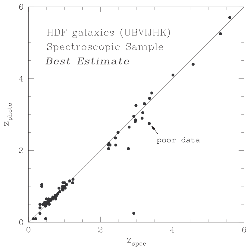
Figure 7.— Our adopted $z_{\rm photo}$ versus $z_{\rm spec}$ for the spectroscopic sample. The galaxy pointed by the arrow has a very poor photometric accuracy.

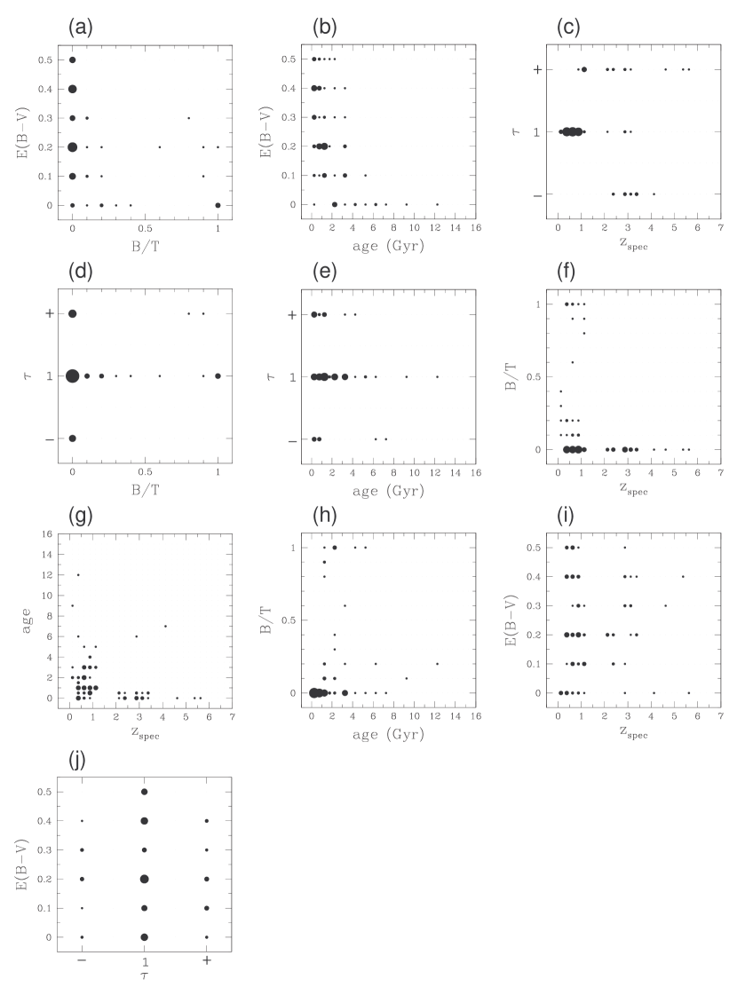
Figure 8.— The parameter distributions of the best-fit SEDs for the spectroscopic sample. The area of the filled circles is proportional to the number of SEDs in the grid. For example, in panel (d) (B/T vs. $\tau$), the grid of (B/T,$\tau$)=(0.0, 1) includes 41 galaxies, the largest circle of all. See the text for details.

Figure 9.— Output $z_{\rm photo}$ versus input $z_{\rm spec}$ of the simulation. The left and right panels are for the 10% and 20% input noises in flux, respectively.

Figure 10.— Comparison of $z_{\rm photo}$ versus $z_{\rm spec}$ among various authors. Results by Sawicki et al. and Gwyn et al. are based on optical 4-band photometry for 74 galaxies with spectroscopic redshifts. Results by Fernández-Soto et al. and this work are based on 7-band photometry for 108 galaxies.

Figure 11.— $z_{\rm photo}$ based on the template SEDs without internal absorption.

Figure 12.— $z_{\rm photo}$ based on the template SEDs using just one value, $\tau_{\it eff}$, for the opacity of intergalactic Lyman absorption.

Figure 13.— $z_{\rm photo}$ obtained based on CWW’s four SEDs as a template set.

Figure 14.— Minimum reduced $\chi^{2}$ obtained with the CWW’s four SEDs as a template set. Compare with Figure 6.

Figure 15.— $N(z)$ of the photometric sample. The solid and dotted lines indicates our results and Fernández-Soto et al.’s.

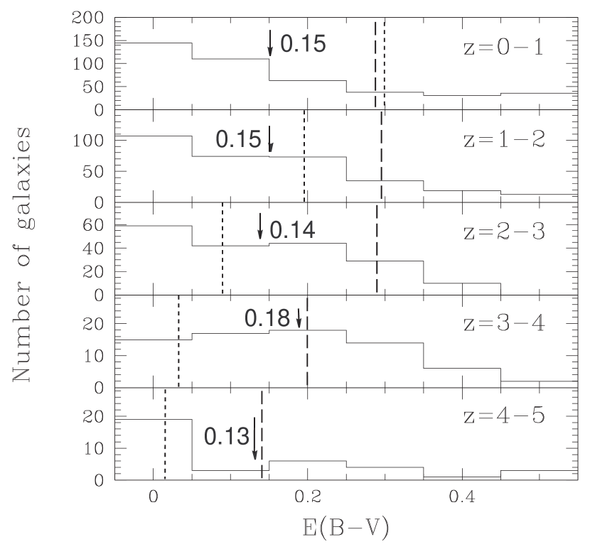
Figure 16.— Histograms of $E(B-V)$ for five redshift bins. Arrows indicate the mean of $E(B-V)$ in each redshift bin. Vertical lines in each bin denote the predictions by Calzetti & Heckman (1999). The dashed lines are for model ‘A’ and the dotted lines are for model ‘B’ (See text for details).

References

- Baum et al. (1963) Baum, W. 1963, IAU Sym. 15: Problems of Extragalactic Research, (New York; Macmillan), p. 390
- Bianchi et al. (1996) Bianchi, L., Clayton, G. C., Bohlin, R. C., Hutchings, J. B., & Massey, P. 1996, ApJ, 471, 203
- Bouchet et al. (1985) Bouchet, P., Lequeux, J., Maurice, E., Prévot, L., & Prévot-Burnichon, M. L. 1985, A&A, 149, 330
- Bohlin, Savage, & Drake (1978) Bohlin, R. C., Savage, B. D., & Drake, J. F. 1978, ApJ, 224, 132
- Bruzual & Charlot (1993) Bruzual, A. G. & Charlot, S. 1993, ApJ, 405, 538
- (6) Bruzual, A. G. & Charlot, S. 1996, GISSEL96, ApJ in preparation
- Cardelli, Clayton, & Mathis (1989) Cardelli, J. A., Clayton, G. C., & Mathis, J. S. 1989, ApJ, 345, 245
- Carlberg et al. (1998) Carlberg R. G., Yee, H. K. C., Morris, S. L., Lin, H., Sawicki, M., Wirth, G., Patton, D., Shepherd, C. W., Ellingson, E., Schade, D., Pritchet, C. J., & Hartwick, F. D. A. 1998, astro-ph/9805131
- (9) Calzetti, D. 1997, AJ, 113, 162
- (10) Calzetti, D. 1997, uulh.conf., 403
- Calzetti & Heckman (1999) Calzetti, D. & Heckman, T. M. 1999, ApJ, 519, 27
- Coleman, Wu, & Weedman (1980) Coleman, G. D., Wu, C., & Weedman, D. W. 1980, ApJS, 43, 393
- Connolly et al. (1995) Connolly, A. J., Csabai, I., Szalay, A. S., Koo, D. C., Kron, R. G., & Munn, J. A. 1995, AJ, 110, 6
- Connolly et al. (1997) Connolly, A. J., Szalay, A. S., Dickinson, M., SubbaRao, M. U., & Brunner, R. J. 1997, ApJ, 486, 11L
- Cowie et al. (1996) Cowie, L. L., Songaila, A., Hu, E. M., & Cohen, J. G. 1996, ApJ, 112, 3
- Cohen et al. (2000) Cohen. J. G. et al. 2000, ApJ submitted, http://www.ifa.hawaii.edu/~cowie/tts/tts.html
- Csabai et al. (1999) Csabai, I., Connolly, A. J., Szalay, A. S., & Budavári, T. 1999, http://tarkus.pha.jhu.edu/~csabai/template/
- Dickinson et al. (1999) Dickinson, M. E. et al. 1999 in preparation, http://www.stsci.edu/ftp/science/hdf/clearinghouse/irim/irim_hdf.html
- Ellis et al. (1996) Ellis R. S., Colless, M., Broadhurst, T., Heyl, J., & Glazebrook, K. 1996, MNRAS, 280, 235
- Fernández-Soto (1999) Fernández-Soto, A. http://bat.phys.unsw.edu.au/~fsoto/hdfcat.html
- Fernández-Soto, Lanzetta, & Yahil (1999) Fernández-Soto, A., Lanzetta, K.M., & Yahil, A. 1999, ApJ, 513, 34
- Fitzpatrick (1985) Fitzpatrick, E. L. 1985, ApJ, 299, 219
- Fitzpatrick (1986) Fitzpatrick, E. L. 1986, AJ, 92, 1068
- Fitzpatrick (1999) Fitzpatrick, E. L. 1999, PASP, 111, 63
- Giallongo et al. (1998) Giallongo, E., D’odorico, S., Fontana, A., Cristiani, S., Egami, E., Hu, E., & McMahon, R. G. 1998, AJ, 115, 2169
- Gordon, Calzetti, & Witt (1997) Gordon, K. D., Calzetti, D., & Witt, A. N. 1997, ApJ, 487, 625
- Gwyn & Hartwick (1996) Gwyn, S.D.J. & Hartwick, F.D.A. 1996, ApJ, 468, 77L
- Hogg et al. (1998) Hogg, D.W., Cohen, J.G., Blandford, R., Gwyn, S.D.J., Hartwick, F.D.A., Mobasher, B., Mazzei, P., Sawicki, M.J., Lin, H., Yee, H.K.C., Connolly, A.J., Brunner, R.J., Csabai, I., Dickinson, M., SubbaRao, M.U., Szalay, A.S., Fernández-Soto, A., Lanzetta, K.M., & Yahil, A. 1998, AJ, 115, 1418
- Kinney, Bohlin, & Calzetti (1993) Kinney, A. L., Bohlin, R. C., & Calzetti, D. 1993, ApJS, 86, 5
- Kinney et al. (1996) Kinney, A.L., Calzetti, D., Bohlin, R.C., & McQuade, K. 1996, ApJ, 467, 38
- Kodama & Arimoto (1997) Kodama, T. & Arimoto, N. 1997, A&A, 320, 41
- Kodama, Bell, & Bower (1999) Kodama, T., Bell, E. F., & Bower, R. G. 1999, MNRAS, 302, 152
- Koo (1985) Koo, D. C. 1985, AJ, 90, 418
- Lanzetta, Yahil, & Fernández-Soto (1996) Lanzetta, K. M., Yahil, A., & Fernández-Soto, A. 1996, Nature, 381, 759
- (35) Lanzetta, K. M., Yahil, A., & Fernández-Soto, A. 1998, AJ, 116, 1066
- Lilly et al. (1995) Lilly, S. J., Tresse, L., Hammer, F., Crampton, D., & Fèvre, O. 1995, ApJ, 455, 108
- Loh & Spillar (1986) Loh, E. D. & Spillar, E. J. 1986, ApJ, 303, 154
- Lowenthal et al. (1997) Lowenthal, J. D., Koo, D. C., Guzmán, R., Gallego, J., Phillips, A. C., Faber, S. M., Vogt, N. P., Illingworth, G. D., & Gronwall, C. 1997, ApJ, 481, 673
- Madau (1995) Madau, P. 1995, ApJ, 441, 18
- Mobasher et al. (1996) Mobasher, B., Rowan-Robinson, M., Georgakakis, A., & Eaton, N. 1996, MNRAS, 282, L7
- Prévot et al. (1984) Prévot, M. L., Lequeux, J., Maurice, E., Prévot, L., & Rocca-Volmerange, B. 1984, A&A, 132, 389
- Sawicki, Lin & Yee (1997) Sawicki, M. J., Lin, H., & Yee, H. K. C. 1997, AJ, 113, 1
- Sawicki & Yee (1998) Sawicki, M. J. & Yee, H. K. C. 1998, AJ, 115, 1329
- Sawicki (1999) Sawicki, M. J. http://www.astro.utoronto.ca/~sawicki/
- Seaton (1979) Seaton, M. J. 1979, MNRAS, 187, 73
- Steidel et al. (1996) Steidel, C. C., Giavalisco, M., Dickinson, M., & Adelberger, K. 1996, AJ, 112, 352
- Wang et al. (1998) Wang, Bahcall, & Turner 1998, ApJ, 116, 2081
- Wang et al. (1999) Wang, Turner, & Bahcall 1999, astro-ph/9906256
- Williams et al. (1996) Williams, R. E., Blacker, B., Dickinson, M., Dxon, V. D., Ferguson, H. C., Fruchter, A. S., Giavalisco, M., Gililand, R. L., Heyer, I., Katsanis, R., Levay, Z., Lucas, R. A., McElroy, D. B., Petro, L., & Postman, M. 1996, AJ, 112, 4
- Yee et al. (1996) Yee, H. K. C., Ellingson, E., Bechtold, J., Carlberg, R. G., & Cuillandre, J. C. 1996, AJ, 111, 1783
- Yee (1998) Yee, H. K. C. 1998, astro-ph/9809347
- (52) Zepf, S. E., Moustakas, L. A., & Davis, M. 1997, ApJ, 474, 1L