The luminosity function of galactic ultra-compact H ii regions and the IMF for massive stars

Abstract

The population of newly formed massive stars, while still embedded in their parent molecular clouds, is studied on the galactic disk scale. We analyse the luminosity function of IRAS point-like sources, with far-infrared (FIR) colours of ultra-compact H ii regions, that have been detected in the CS(2–1) line - a tracer of high density molecular gas. The FIR luminosities of 555 massive star forming regions (MSFRs), 413 of which lie within the solar circle, are inferred from their fluxes in the four IRAS bands and from their kinematic distances, derived using the CS(2–1) velocity profiles. The luminosity function (LF) for the UCH ii region candidates shows a peak well above the completeness limit, and is different within and outside the solar circle (96% confidence level). While within the solar circle the LF has a maximum for $2\,10^{5}\,L_{\odot}$, outside the solar circle the maximum is at $5\,10^{4}\,L_{\odot}$. We model the LF using three free parameters: $-\alpha$, the exponent for the initial mass function (IMF) expressed in $\log(M/M_{\odot})$; $-\beta$, the exponent for a power law distribution in $N^{\star}$, the number of stars per MSFR; and $N^{\star}_{\mathrm{max}}$, an upper limit for $N^{\star}$. While $\alpha$ has a value of $\sim 2.0$ throughout the Galaxy, $\beta$ changes from $\sim 0.5$ inside the solar circle to $\sim 0.7$ outside, with a maximum for the number of stars per MSFR of $\sim$650 and $\sim$450 (with $1\leq M/M_{\odot}\leq 120$). While the IMF appears not to vary, the average number of stars per MSFR within the solar circle is higher than for the outer Galaxy.

1 Introduction

A new tool is now available to probe the population of recently formed massive stars, while still embedded in their parent clouds. Such stars are surrounded by a compact H ii region, with an ionization front working outwards into the cloud. Regions undergoing massive star formation contain one or more ultra-compact H ii (UCH ii) regions, and possibly more evolved H ii regions. Bronfman et al. (1996, BNM) completed a survey in CS(2–1) towards IRAS point sources satisfying the Wood & Churchwell (1989a) far-infrared (FIR) colour criteria for UCH ii regions. The CS molecule is a tracer of high density molecular gas; a CS(2–1) detection strengthens the UCH ii region identification and provides kinematic information. BNM detected 843 sources (hereafter IRAS/CS sources), whose azimuthally averaged galactic distribution is presented in Bronfman et al. (2000, BCMN). In this work we construct the luminosity function (LF) for the IRAS/CS sources, and show that it presents significant variations with galactocentric radius. We interpret the shape of the IRAS/CS sources LF and its variations in terms of an ensemble of massive star forming regions. The stellar content of IRAS/CS sources is characterised by the number of stars and their mass spectrum which, because of the youth of the systems, is taken to represent closely their initial mass function (IMF).

The use of young tracers to derive the IMF minimises the dependence on modelling, which afflicts most previous studies. The standard approach to determining the high mass end of the IMF has been through O and B star counts in the solar neighbourhood (e.g. Miller & Scalo 1979, Lequeux 1979). The average mass spectrum of newly formed stars is taken as a power law, and the value of the exponent characterises the IMF. These approaches require assumptions on the star formation history, and have the drawback of not probing the whole galactic disk. Garmany et al. (1982) addressed the question of large scale variations in the IMF exponent, and they favour a decrease with galactocentric radius (although their result has been reinterpreted, e.g. Massey 1998). A different tool was used by Vázquez & Feinstein (1989), who linked the variations in the open cluster luminosity function (Burki 1977) to variations in the IMF index.

Young objects such as H ii regions have also been used to study massive stars in the galactic context. McKee & Williams (1997, MW97) characterised the population of newly formed massive stars through the luminosity function of OB associations. The ionising luminosity absorbed by the gas surrounding OB associations can be traced through the radio flux of H ii regions, and the frequency distribution in luminosity of H ii regions is in turn a function of the number of exciting stars and their masses. However, MW97 a-priori fixed the shape of the IMF and the distribution for the number of exciting stars. This method is also strongly model dependent due to the lack of complete information on galactic H ii regions, and the fact that the population of H ii regions is not homogeneous in age. Comerón & Torra (1996, CT96) also analysed the galactic disk distribution of newly formed massive stars, through a sample of IRAS point sources with colours of UCH ii regions. But they did not use kinematic information to derive the galactic distribution of the UCH ii regions, and their work is based on a position-independent LF.

The aims of this work are to present the FIR LF of massive star forming regions still embedded in their parent clouds; to investigate the LF large scale variations; and to analyse the LF in terms of the embedded stars’ mass spectrum. In Sect. 2 we construct the LF of IRAS/CS sources for different sectors in the galactic disk, and show that it presents significant variations with galactocentric radius. In Sect. 3 we analyse the stellar population underlying the IRAS/CS sample through a simple model based on a synthetic ensemble of massive star forming regions (MSFRs). A search in parameter space is conducted in Sect. 4. The results of this analysis and the questions of the number and the mass spectrum of stars per MSFR will be addressed in Sect. 5. In particular, we will show that the mass spectrum of newly formed massive stars is constant across the galactic disk, although the average number of stars per MSFR is lower outside the solar circle. Section 6 is a brief estimate of the fraction of lifetime O stars spend in the embedded phase. In Sect. 7 we summarise our conclusions.

2 FIR luminosity function of UCH ii regions

The velocity information provided by the CS(2–1) observations from BNM allows, through the adoption of a rotation curve, to derive their galactocentric distances, and hence their heliocentric distances and luminosities. The galactic disk is assumed to be in circular motion, with $R_{\circ}=8.5\,$kpc and $V_{\odot}=220$ km s^-1. For the region of the Galaxy outside the solar circle (outer Galaxy) the procedure is a simple coordinate transformation from galactic longitude, latitude and velocity ($l,\,b,\,V_{\rm lsr}$) to galactocentric radius, height over the plane and azimuth ($R,\,z,\,\theta$). But such a transformation is bivalued for the region within the solar circle (inner Galaxy). There is a heliocentric distance ambiguity such that, unless a source lies just on the subcentral point (the tangent point to a galactocentric ring for a given longitude), there are two points along the line of sight, at the same distance on both sides of the subcentral point, that have the same line of sight velocity.

The method we used to resolve the distance ambiguity is described in BCMN. It is a statistical method that consists in weighting the near and far distances with a normal distribution in height over the galactic plane. Each source is assigned an effective luminosity, which is the weighted average of the near and far luminosities. The centroid and width of the vertical distribution, $Z_{\circ}(R)$ and $Z_{\frac{1}{2}}(R)$, are determined through an iterative process for galactocentric bins $0.1\,R_{\circ}$ wide. A consistency check for this method can be found below in this Section.

The kinematic distances are not reliable in the direction of the galactic centre, and also when the line of sight velocities are of the same order as the non-circular velocity components. Therefore, we excluded from the present analysis all sources within $\pm 10^{\circ}$ of the galactic centre, and within $\pm 5^{\circ}$ of the galactic anti-centre, as well as sources with $|V_{\rm lsr}|\leq 10\,{\rm km}\,{\rm s}^{-1}$. The resulting range in galactocentric radius, where the disk is properly sampled, excludes the solar circle. We restricted the analysis to sources with $0.3\leavevmode\nobreak\ \leq R/R_{\circ}\leq 0.9$ and $1.1\leq R/R_{\circ}\leq 1.6$.

The sources close to the subcentral points are an important consistency check of our method to resolve the distance ambiguity within the solar circle. The kinematic distance of a source at the subcentral point and in pure circular motion about the galactic centre is uniquely determined. The subcentral sources sample was defined as the subset with line of sight velocities no more than 10  km s^-1 different in absolute value from the terminal velocity (the maximum velocity expected for a given longitude in the case of circular rotation).

We estimate the far infrared flux of an IRAS/CS source by summing over the four IRAS bands,

$$F_{IRAS}=\sum_{j=1}^{4}\,\nu\,F_{\nu}(j),$$ (1)

where $F_{\nu}(j)$ are the IRAS band flux densities, as listed in the IRAS Point Source Catalog (1985). In order to test this approximation we compared with the total fluxes reported for 53 UCH ii regions by Wood & Churchell (1989b, WC89, their Tables 17 and 18). Figure 1a shows the ratio of the $F_{IRAS}$ fluxes (obtained by Eq. 1) to the total fluxes of WC89 (which are integrated up to 100$\,\mu$m), as a function of $F_{IRAS}$. Equation 1 overestimates the WC89 fluxes by about a constant 20%, but WC89 did not include a correction for the 100$\,\mu$m – 1 mm flux, which they estimate could be as high as 50%. We thus expect Eq. 1 to be a good estimate of the total luminosity of IRAS/CS sources within 30% (50% – 20%).

Since we will average the luminosity function of UCH ii regions over large areas of the galactic disk, it is important to estimate the minimum luminosity above which the disk is properly sampled. The lowest flux $F_{IRAS}$ in the sample, $F_{IRAS}=6\,10^{-13}$ W m^-2, corresponds to $\log(L_{\mathrm{min}}/L_{\odot})=3.6$ at a distance of 15 kpc. Figure 1b shows a histogram of the total number of sources in our sample as a function of $F_{IRAS}$ (without the velocity filter $|V_{\rm lsr}|\leq 10\,{\rm km}\,{\rm s}^{-1}$). The triangles show the fraction of sources with only upper limits in the 100$\,\mu$m band (right hand scale). Could a significant number of sources be missed by IRAS near the minimum detected flux? A lower $F_{IRAS}$ sensitivity would be hinted at by an increased fraction of upper limits in the reported IRAS fluxes, which is not the case. However, the higher far-IR background towards the central regions of the Galaxy results in a completeness limit of $\log(L_{\mathrm{min}}/L_{\odot})=4.5$ at 8.5 kpc, within $-10<l<10$, $-0.3<b<0.3$. But over a broader longitude range, $\log(L_{\mathrm{min}}/L_{\odot})=4.0$ at 8.5 kpc, within $-60<l<60$, $-0.3<b<0.3$. As the luminosity functions of the subcentral sources (which are all within 8.5 kpc of the Sun) is in good agreement with that of the whole inner Galaxy (see below), we take $\log(L_{\mathrm{min}}/L_{\odot})=4$ as the completeness limit of the IRAS/CS sample.

Figure 1: a) The ratio of the fluxes published by WC89 to $F_{IRAS}$, as a function of $F_{IRAS}$ in 10^-9 W m^-2. b) The number of sources (left hand scale) as a function of $F_{IRAS}$ in 10^-9 W m^-2. The proportion of sources with an upper limit in the 100$\,\mu$m band is shown in triangles (right hand scale)

The LF of the whole sample of IRAS/CS sources, our main observational result, appears to be significantly different inside and outside the solar circle; in Fig. 2 we distinguish between $R<R_{\circ}$ and $R>R_{\circ}$. The LFs cover a very wide range in luminosity, over three orders of magnitude, which allows using logarithmic luminosity bins corresponding to a factor of 300%. Within the solar circle the LF obtained using the effective luminosities is confirmed to be a good estimate of the actual LF through its close similarity with the LF of the sources near the subcentral points, shown in dotted line. For comparison, placing all the sources at the ‘near’ or ‘far’ kinematic distance changes the peak of the LF as a function of logarithmic luminosity from 4.25 to 5.75, while the LF obtained using the effective luminosities peaks at 5.25. The good match with the subcentral source sample LF lends strength to a comparison of the luminosity functions between the outer and inner Galaxy, based on the effective luminosities. We will refer to the luminosity functions for the whole inner and outer Galaxy by LFⁱⁿ and LF^out.

Figure 2: The luminosity function for galactic UCH ii regions, from the IRAS/CS sample. The whole disk was divided at the solar circle, the upper and lower plots correspond to the inner and outer Galaxy LFs, computed with 413 and 142 sources respectively. In the upper plot the inner Galaxy LF derived from the effective luminosities is shown in solid line, while the thick dotted line is the LF for sources near the subcentral points (57 sources). The distributions in these plots are normalised so that the areas under the histograms is one over $\log(L/L_{\odot}$)$>$4. Shot noise gives 1-$\sigma$ error bars on the subcentral LF of $\sim$25%

The dominant source of uncertainty in the LF is shot noise. The errors in the galactic disk surface FIR luminosity amount to about 10% upwards, 20% downwards (Fig. 3 in BCMN). The fractional error on the FIR surface luminosity represents the typical fractional error on the luminosity of one source. These errors stem from the IRAS 100$\,\mu$m band flux uncertainty, coupled with the kinematic distance uncertainty due to non-circular motions of about 5 km s^-1. Adding in quadrature the 30% uncertainty related to the use of Eq. 1, we have an average error on the luminosity of a source of at most 36%. Compared to the 300% width of the luminosity bins, a 36% uncertainty is negligible, apart from a slight smoothing effect without practical consequence.

The differences in the LFs inside and outside the solar circle are statistically significant. As a statistic for the difference between the inner and outer LFs, we used a $\chi^{2}$ test which has the following expression in this context,

$$\chi^{2}=\sum_{i}\frac{({\rm LF}^{\mathrm{in}}_{i}-{\rm LF}^{\mathrm{out}}_{i})^{2}}{\frac{{\rm LF}^{\mathrm{in}}_{i}}{(N_{\mathrm{in}}{\Delta}\log L)^{2}}+\frac{{\rm LF}^{\mathrm{out}}_{i}}{(N_{\mathrm{out}}{\Delta}\log L)^{2}}},$$ (2)

where we sum over the bins above the luminosity limit of 10${}^{4}\,L_{\odot}$. The result is $\chi^{2}=11.4$, or that LFⁱⁿ and LF^out are different at a significance level of 95.6% (with a $\chi^{2}$ distribution for 5 degrees of freedom, corresponding to the number of bins with non-zero counts above the luminosity limit). For comparison, the same test applied to the northern and southern LFs inside the solar circle gives a probability of 45% that the distributions are different, so they are comparable relative to the differences between the LFs inside and outside the solar circle. Another application of this statistical test gives that LFⁱⁿ and the subcentral source LF are the same at a confidence level of 87%.

We emphasize the presence of a peak in the LF of IRAS/CS sources, well above the completeness limit. The strongest evidence in that sense can be found in the LFs for the outer Galaxy and for the subcentral sources, where the $L_{\mathrm{min}}$ completeness limits are lowest. The shape for the LF we report is quite different from a power law functional form (e.g. as used in CT96).

3 Synthetic fits to the IRAS/CS luminosity function

One immediate consequence of the shape of the IRAS/CS luminosity function is that these sources are better understood as clusters of stars rather than in the framework of one dominant star per source. A single exciting star would result in a power law LF: an IMF index $\alpha$ (see below), and mass-luminosity relation $L\propto M^{\gamma}$, give a probability distribution in luminosity $p(L)\propto L^{-\frac{\alpha+\gamma}{\gamma}}$.

We used a simple model to examine whether the variations in the LFs of IRAS/CS sources from inside to outside the solar circle can be traced to the underlying young stellar population. We proceed to describe a Monte Carlo analysis for the ensemble of massive star forming regions in the galactic disk. The luminosity of a MSFR is the sum of the luminosities of each star, given by the mass-luminosity relationship. We used a polynomial fit to the mass-luminosity relation of the tracks presented in Schaller et al. (1992) for Z=0.02, at the first time step they list,

$$\log(L/L_{\odot})=-0.127+4.656\,\log(M/M_{\odot})$$ (3)

$$-0.764\,\log^{2}(M/M_{\odot}).$$

The metallicity dependence of the mass-luminosity relation was neglected, as the Z=0.001 tracks in Schaller et al. (1992) have luminosities within 10% of Eq. 3 for $M\,>\,7\leavevmode\nobreak\ M_{\odot}$.

The synthetic population of MSFRs was generated in the following way. The number of stars in a given MSFR, $N_{\star}$, is generated randomly within the range $1\leq N_{\star}\leq N^{\mathrm{max}}_{\star}$, and subject to a power law probability distribution with exponent $-\beta$, $p(N_{\star})\propto N_{\star}^{-\beta}$. A discussion of the model sensitivity on $N^{\mathrm{max}}_{\star}$ will be found in Sect. 4. Given $N_{\star}$, the total luminosity of a MSFR is calculated by summing the individual luminosities of each star, using the mass-luminosity relationship. The mass of each star is generated randomly, within the range $1\leq M/M_{\odot}\leq 120$ and satisfying the IMF distribution,

$$p(M)\propto M^{-(1+\alpha)};$$ (4)

in this notation the Salpeter (1955) IMF corresponds to $\alpha=1.35$. Thus the luminosity of each MSFR is randomly generated with $L_{\rm MSFR}=\sum_{i=1}^{N_{\star}}L(M_{i})$, and an ensemble of 5000 MSFRs provides a population large enough to compute the synthetic luminosity function (that this is one order of magnitude larger than the number considered in the observed LF does not affect the results, only helps to reduce the random fluctuations).

An important simplification in this approach is that the ensemble of MSFRs is assumed to be homogeneous in age (see Sect. 6). Furthermore, it should be mentioned before discussing the results of the model that the mass-luminosity relation remains mainly theoretical for massive stars. Although Burkholder et al. (1997) give observational evidence that support the massive star models up to $25\,M_{\odot}$, the upper mass limit we used is $120\,M_{\odot}$, where to our knowledge no direct observational information exists to back the theoretical models.

4 Search in parameter space and the role of $N\mathrm{{}^{max}_{\star}}$

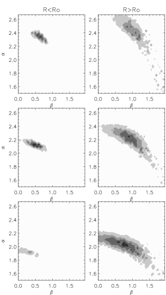
A first broad search for the parameters $\alpha$ and $\beta$ requires specifying $N\mathrm{{}^{max}_{\star}}$. It could be thought firsthand that any value of $N\mathrm{{}^{max}_{\star}}$ high enough to simulate infinity would do, but we tried $N\mathrm{{}^{max}_{\star}}=10000$ and did not obtain any fit, over the range $1.5<\alpha<2.7$ , $0<\beta<2$. We distinguished three cases, fixing the maximum number of stars per MSFR, $N\mathrm{{}^{max}_{\star}}$, to 500, 1000 and 2000. Figure 3 shows the $\chi^{2}$ cumulative probability for the goodness of fit as a function of parameter space. In the observed IRAS/CS LF, we have five bins with non-zero counts above the completeness limit of 10${}^{4}\,L_{\odot}$. The number of degrees of freedom is thus 3, which corresponds to the five bins in comparison less two free parameters ($\alpha$ and $\beta$). The fit to LF^out is a lot more noisy, a consequence of the reduced number of IRAS/CS sources used to compute the LF.

It is apparent that for any value of $N\mathrm{{}^{max}_{\star}}$, $\alpha$ is similar inside and outside the solar circle, while the acceptable values for $\beta$ are markedly different. It can also be noticed from Fig. 3 that the best fit $\beta$ are rather independent of $N\mathrm{{}^{max}_{\star}}$, in contrast with the behaviour of the best fit IMF index $\alpha$. For $N\mathrm{{}^{max}_{\star}}=1000$, the IMF index in the inner Galaxy, at 50% confidence level for the goodness of fit (with two free parameters), corresponds to $2.05\leq\alpha\leq 2.15$. This is very close to the result for the outer Galaxy, $2.1\leq\alpha\leq 2.3$. The case where $N\mathrm{{}^{max}_{\star}}=500$ seems to give better results for $R>R_{\circ}$, and constrains $1.9<\alpha<2.15$ at 50% confidence. This range of values, $\Delta\alpha=0.1$ for $R<R_{\circ}$ and $\Delta\alpha=0.15$ for $R>R_{\circ}$, will be used as an indication of the uncertainty level in the best fit $\alpha$.

Figure 3: Search in ($\alpha,\beta$) parameter space for the best fit model, with three guesses for $N\mathrm{{}^{max}_{\star}}$. Plotted is the $\chi^{2}$ cumulative probability for the goodness of fit (with 2 free parameters), with contours at 10%, 30%, 50% and 70%. The upper two plots were computed with $N\mathrm{{}^{max}_{\star}}=2000$, the middle two with $N\mathrm{{}^{max}_{\star}}=1000$, and the bottom two with $N\mathrm{{}^{max}_{\star}}=500$

As the distribution of $N_{\star}$ seems to be a bounded power law, there exists a maximum for the number of stars born in a MSFR within a finite mass range. It should be kept in mind that the total number of stars could in fact depend on the stellar masses and the star formation history of a MSFR; we expect the parameter $N_{\star}$ to synthesise more complex processes. Observational constraints to fix $N\mathrm{{}^{max}_{\star}}$ are difficult to find, because stellar censuses are available only for much larger regions like OB associations, open clusters, or longer lived H ii regions.

5 The IMF index and possible large scale variations

After finding reasonable values for $N\mathrm{{}^{max}_{\star}}$, we extend the search to include all three parameters, and obtain

$$(\alpha,\beta,N\mathrm{{}^{max}_{\star}})= (1.988,0.49,646), {\rm for}\leavevmode\nobreak\ R<R_{\circ},\leavevmode\nobreak\ {\rm and}$$ (5)

$$(\alpha,\beta,N\mathrm{{}^{max}_{\star}})= (1.991,0.73,450), {\rm for}\leavevmode\nobreak\ R>R_{\circ}.$$

Thus the best fitting sets of parameters have $\alpha=2.0$. Values for the significance of the fits are $\sim 60\%$, with two degrees of freedom (5 bins in comparison less 3 free parameters). Figure 4 shows the models that best fit the LFs. Due to the Monte Carlo approach, secondary $\chi^{2}$ minima are found about the true minimum. Multiple minimization runs with various initial guesses fluctuate about the above values: from $(1.98,0.57,708)$ to $(2.03,0.40,748)$ for $R<R_{\circ}$.

Keeping $N\mathrm{{}^{max}_{\star}}$ fixed at the best fit value, with the $\Delta\alpha$ uncertainties quoted in the previous section (i.e. above a 50% confidence level in a 2-D slice), our best values for $\alpha$ are $1.95<\alpha<2.05$ in the inner Galaxy, and $1.9<\alpha<2.15$ in the outer Galaxy.

As an indication of the uncertainty level related to the use of Eq. 1, increasing the bolometric fluxes to $2\,F_{IRAS}$ results in $(\alpha,\beta,N\mathrm{{}^{max}_{\star}})=(1.72,0.29,457)$ for $R<R_{\circ}$. Only very low significance fits were found using either $5\,F_{IRAS}$, or $0.5\,F_{IRAS}$. A factor of 2 in the mass-luminosity relation $L(M)$ gives $(\alpha,\beta,N\mathrm{{}^{max}_{\star}})=(2.005,0.48,700)$, i.e. no significant change. A steep IMF index seems to be a robust result of our analysis.

Figure 4: Best fit models (dotted lines) to the inner and outer Galaxy IRAS/CS LFs (solid lines), above the completeness limit $\log(L/L_{\odot})=4$. In ordinates is the LF normalised over $\log(L/L_{\odot})\geq 4$, as a function of $\log(L/L_{\odot})$

The IMF index $\alpha$ for the inner and outer Galaxy seems to be the same, although $\beta$ changes significantly. In other words, although the average mass of newly formed stars is the same inside and outside the solar circle, the average number of stars per star forming region and in a finite mass range is lower in the outer Galaxy. The best fits of the parameter $\beta$ imply that the expectation value for the number of stars per MSFR with $1\leq M/M_{\odot}\leq 120$, $<N>$, decreases from 225 for $R<R_{\circ}$ to 120 for $R>R_{\circ}$. The decrease in $<N>$ is not an effect related to the area covered by the 100$\,\mu$m IRAS beam: due to the lower FIR background towards the outer Galaxy, the IRAS point sources are detected to greater distances than in the inner Galaxy (the average distance to IRAS/CS sources is 6.92 kpc for the outer Galaxy, and 5.32 kpc in terms of the effective distances for the inner Galaxy).

Is there a gradient in the IMF index with galactocentric radius? How does our value for the IMF index compare with other estimates? The gradient proposed by Garmany et al. (1982) has been re-interpreted as a result of contamination from field O stars (Massey et al. 1995a), which seem to derive from a very steep IMF. The values Massey et al. (1995b) and Massey (1998) quote for $\alpha$ in the Milky Way and the Magellanic Clouds OB associations are $1.1\pm 0.1$ and $1.3\pm 0.1$, which argues against a metallicity dependence of $\alpha$, at least over 10 -120 $M_{\odot}$. But constraining the analysis to nearby OB associations gives steeper values, Claudius & Grosbøl (1980) give $\alpha=1.9$ over 2.2 -10 $M_{\odot}$, and Brown (1998) gives $\alpha$=1.9 for the Upper Scorpius subgroup of Sco OB2, over 3 -16 $M_{\odot}$. Brown (1998) used Hipparcos data to ascertain membership (see de Zeeuw et al. 1999), which is crucial in the coeval approximation; the very large OB associations in Massey et al. probably have a complex star formation history. Although Massey et al. establish a good case for a universal massive star IMF, the exact value of the IMF index is still an open issue. Our contribution to this debate is that there certainly are differences in the physical processes governing star formation in the outer spiral arms and the molecular ring. In our simple approach, and understanding that we restricted our study to regions of massive star formation embedded in dense molecular cores and with at least one UCH ii region, it seems that although the IMF index is constant, the average number of stars born per region is lower outside the solar circle. We favour a rather steep IMF index, close to the values from Brown (1998).

6 Lifetime of UCH ii regions

UCH ii regions are fairly short lived in comparison with giant H ii regions. Wood & Churchwell (1989a) estimated the lifetimes of UCH ii regions by comparing the number of O stars in the solar neighbourhood (Conti et al. 1983) and the number of IRAS point sources that match the IRAS colours of UCH ii regions. They conclude that 10% to 20% of an O star’s main sequence lifetime is spent embedded in a molecular cloud, in the UCH ii phase. This fraction has been reevaluated to only 0.5% by CT96, and our estimate is $\leq 2\%$ (see below). Under the assumption that the luminosity of a MSFR is dominated by the most massive star, CT96 show that if there is a variation of UCH ii lifetime with stellar mass, it is not as significant as the uncertainties in the IMF. The crossing time at 10 km s^-1 is 10⁴ yrs for a typical UCH ii region (i.e. G34.3+0.2, which at a distance of 3.7 kpc is about $5\,10^{17}\,$cm). Thus the margin between the dynamical timescale and the time O stars spend in the embedded phase of $<10^{5}$ yrs is narrow, and can be affected by many parameters other than the mass of the most massive star, such as clumpiness of the molecular clouds and relative motions between the exciting star and the molecular clumps. It is unlikely that the lifetimes of UCH ii regions depend strongly on their stellar contents.

From our synthetic population of MSFRs, we find that the average number of O stars per MSFR, with luminosities in excess of $L(20\,M_{\odot}$), is 0.55 for $R<R_{\circ}$ and 0.29 for $R>R_{\circ}$ - we will consider 0.5 O stars per IRAS/CS source. Within 2.5 kpc of the Sun, Conti et al. (1983) report 436 O stars with $M>20\,M_{\odot}$. We have 15 IRAS/CS sources above the luminosity limit $L(20\,M_{\odot}$) (counting all sources, outside the cuts in longitude described in Sect. 2 but including the sources with $|V_{\mathrm{lsr}}|\leq 10\leavevmode\nobreak\ {\rm km\,s}^{-1}$). The average fraction of lifetime spent in the embedded phase would thus be $0.5\times 15/(436+0.5\times 15)=0.017$. Alternatively, counting the IRAS/CS sources with galactocentric radii within 0.9 to $1.1\,R_{\circ}$, we have 40 sources more luminous than $L(20\,M_{\odot}$), distributed over an area of 80.5 kpc² (BCMN). This would give 9.8 IRAS/CS sources within 2.5 kpc of the Sun. The average fraction of lifetime O stars spend in the embedded phase would thus be $0.5\times 9.8/(436+0.5\times 9.8)=0.011$. This latter approach has the advantage of not suffering as much from the peculiar velocities of local sources. But some O stars in the transition between the embedded UCH ii phase and the field stars could have been missed by Conti et al. (1983). Therefore we estimate that O stars spend $\leq 2\%$ of their lifetime in the embedded phase.

7 Conclusions

We have constructed the FIR luminosity function for IRAS point sources with colours of UCH ii regions and CS(2–1) detections, for different sectors in the galactic disk. The LFs are reliable above a luminosity of $10^{4}\leavevmode\nobreak\ L_{\odot}$, and extend to $\sim 10^{6}\leavevmode\nobreak\ L_{\odot}$ in the high luminosity end, with a peak at $\sim 10^{5}\leavevmode\nobreak\ L_{\odot}$. We analysed the trends in the LF of IRAS/CS sources in terms of an ensemble of massive star forming regions, and two free parameters suffice to provide a remarkably good fit to the shape of the LF. The fits required a maximum for the number of stars born in a given MSFR with $1\leq M/M_{\odot}\leq 120$. The best results were obtained setting $N\mathrm{{}^{max}_{\star}}=646$ for $R<R_{\circ}$, and $N\mathrm{{}^{max}_{\star}}=450$ for $R>R_{\circ}$. A few conclusions can be summarised:

1. The LFs inside and outside the solar circle are different at 96% confidence level. The LF within the solar circle, built with 413 sources, peaks at $2\,10^{5}L_{\odot}$, while the LF outside the solar circle, built with 142 sources, peaks at $5\,10^{4}\,L_{\odot}$.

2. The IMF index we obtain is $\alpha=2$ and constant with galactocentric radius. At 50% cumulative probability for the goodness of fit, and keeping $N\mathrm{{}^{max}_{\star}}$ fixed at the best fit value, $1.95<\alpha<2.05$ in the inner Galaxy, and $1.9<\alpha<2.15$ in the outer Galaxy.

3. A power law distribution for the number of stars per MSFR has an exponent $-\beta\sim-0.49$ in the inner Galaxy. But in the outer Galaxy the best fit model corresponds to $-\beta\sim-0.73$. Thus, the expectation value for the number of stars per MSFR with $1\leq M/M_{\odot}\leq 120$ decreases from 225 for $R<R_{\circ}$ to 120 for $R>R_{\circ}$.

The results of our analysis show that the observed luminosity functions for UCH ii regions can be traced to the underlying young population. The differences within and outside the solar circle reflect a decrease in the average number of stars per massive star forming region towards the outer Galaxy, rather than a steeper IMF.