(Teff,log g,[Fe/H]) Classification of Low-Resolution Stellar Spectra using Artificial Neural Networks

Abstract

New generation large-aperture telescopes, multi-object spectrographs, and large format detectors are making it possible to acquire very large samples of stellar spectra rapidly. In this context, traditional star-by-star spectroscopic analysis are no longer practical.  New tools are required that are capable of extracting quickly and with reasonable accuracy important basic stellar parameters coded in the spectra.  Recent analyses of Artificial Neural Networks (ANNs) applied to the classification of  astronomical spectra have demonstrated the ability of this concept to derive estimates of  temperature and luminosity. We have adapted the back-propagation ANN technique developed by von Hippel et al. (1994) to predict effective temperatures, gravities and overall metallicities from  spectra with resolving power $\lambda/\delta\lambda\simeq 2000$ and low signal-to-noise ratio. We show that ANN techniques are very effective in executing a three-parameter (Teff,log g,[Fe/H]) stellar classification. The preliminary results show that the technique is even capable of identifying outliers from the training sample.

McDonald Observatory and Department of Astronomy, The University of Texas at Austin RLM 15.308, Austin, TX 78712-1083, USA

Gemini Observatory, USA

Department of Physics and Astronomy, Michigan State University, East Lansing, MI 48824, USA

McDonald Observatory and Department of Astronomy, The University of Texas at Austin RLM 15.308, Austin, TX 78712-1083, USA

Instituto Astronomico e Geofisico, Universidade de Sao Paulo, Av. Miguel Stefano 4200, 04301-904, Sao Paulo, SP, Brazil

1. Introduction

Artificial Neural Networks (ANNs) have been  applied to the classification of stellar spectra very recently, but with great success. These computational systems provide a mapping from a set of inputs to a set of desired outputs and can be  trained to classify  anything with great accuracy and speed. Vieira & Ponz (1995) made use of this technique to carry out the spectral classification  of low-resolution spectra obtained by the IUE satellite. They found that ANNs performed better than classical methods based on a defined metric distance, making it possible an accuracy of 1.1 spectral subclasses. More recently, Bailer-Jones et al. (1998) trained an ANN to classify objective-prism spectra from the Michigan Spectral Survey, extracting the spectral type (std. deviation = 1.09) and the luminosity class (success rate $>$ 95%).

We have stepped forward from the two-dimensional (temperature and luminosity class) classification to the three-dimensional, including the stellar metal content. We have made use of part of the observational material collected by Beers and his large collaborative projects (Beers et al. 1999). Table 1 summarizes the main characteristics of the spectra and the acquisition places.

Table 1.: Origen and description of the spectra employed in the study

	Telescope	Detector	Coverage (Å)	Å/pix
	Mount Stromlo Observatory 1.9 m	PCA	3750-4100	0.4
	Siding Spring Observatory 2.3 m	PCA	3800-4300	0.5
	Siding Spring Observatory 2.3 m	Loral 1024$\times$1024	3800-4400	0.5
	Siding Spring Observatory 2.3 m	SITe 1752$\times$532	3750-4600	0.5
	Las Campanas 2.5 m	Reticon	3700-4500	0.3 (0.65)
	2D-FRUTTI	0.6 (0.65)
	Palomar 5 m	Reticon	3700-4500	0.3 (0.65)
	2D-FRUTTI	0.6 (0.65)
	European Southern Observatory 1.5 m	Ford 2048$\times$2048	3750-4750	0.65
	European Southern Observatory 1.5 m	Loral 2048$\times$2048	3750-4600	0.5
	Kitt Peak National Observatory 2.1 m	Tek 2048$\times$2048	3750-5000	0.65
	Isaac Newton 2.5 m	Tek 1024$\times$1024	3750-4700	0.9
	Lowell Observatory 1.8 m	Tek 512$\times$512	4000-4250	1.0
	Observatoire Haute-Provence 1.9m	Tek 512$\times$512	3750-4250	0.9

2. Input data

A selection of 182 stars spanning all metallicites, gravities and effective temperatures (Teffs) was selected for training. ANNs can over-learn, that is, they may get to the level of taking into account features that are particular to the stars in the training sample, rather than typical characteristics of the spectral classes, gravities, and metallicities they represent. For this reason, an independent sample must be used to check that the net is properly classifying the stars. 82 stars were used for this purpose. Figure 1 shows the distribution of the metallicity of the training and testing samples.

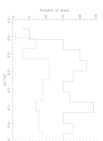
Figure 1.: Distribution of metallicities in the training (blue) and testing (red) samples

The training and testing samples were selected to make sure that the mapping of the Teff-logg was adequate as well, as demonstrates Figure 2.

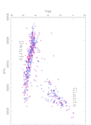
Figure 2.: Distribution of the training (blue) and testing (red) samples across the HR diagram

Metallicities for the testing and training samples were compiled by Beers et al. (1999). Effective temperatures have been derived  from compiled B-V colors, applying the calibrations of Alonso et al. (1996) for dwarfs and subgiants, and Alonso et al. (1999, private communication) for more evolved stars. These calibrations are based on the InfraRed Flux Method, developed by Blackwell and collaborators (e.g., Blackwell & Lynas-Gray 1994). We have taken advantage of the distance estimates made by  Beers et al. (1999) (spectroscopic parallaxes) to interpolate in the evolutionary isochrones of Bergbush & VandenBerg (1992) and derive bolometric corrections and masses. The calculated luminosities were combined with the effective temperatures to obtain the stellar radii, and then with the masses to estimate the gravities.

3. Spectra processing

Before entering the ANN, the spectra were pre-processed using IRAF routines. They were first continuum flattened, using a 3rd order spline interpolation method. Then, the spectra were shifted to a pre-chosen template velocity by the “Fxcor” and “Dopcor” packages and rebinned to a common dispersion (0.646 Å/pix). Finally, using “Wspectext” , the spectra were converted into text format.

4. Applying the neural network

All weights are initially random. A node fires at a value given by a sigmoid function, F(a) = 1/(1+e-a), where a = $\Sigma$ (wij x Ii),where wij is the corresponding weight and Ii the corresponding input. Then F(a) = Oj, the hidden (or output) node value.

The weight training is accomplished by means of the Ripley code (Ripley 1993), a quasi-Newtonian optimization method.  Besides the initial random weights, Ripley’s code eliminates all free parameters that are present in most back propagation networks (e.g. learning rate, momentum term).

Artificial Neural Networks of 3, 5, 7, and sometimes 9 and 11 hidden nodes were tried with varying random weight initializations. The net architecture finally  used is 1 hidden layer and 5 hidden nodes, which produced the most reasonable results based on overdetermination as well as reliability and time constraints.  A typical training session involved about 1000 iterations in perhaps 30 minutes on a Sun ultra 30. This implies a testing time of much less than 1 second per spectrum.

We chose a final spectral range of 3630 to 4890 Å before running the ANN to ensure the best spectral quality possible. At 0.646 Å/pix, this yields 1952 spectral resolution elements, i.e. input values, per spectrum.

5. Results and conclusions

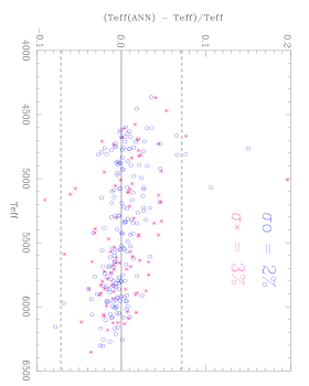
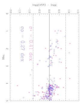
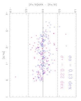
Figure 3.: Deviation of the ANN answers from the assumed parameters for the training (blue) and testing (red) samples

Our results are displayed in Figure 3. Several stars in the training sample were indicated by the net as problematic. A close look to those outliers revealed that an important number of them corresponded to obvious errors in the application of the spectroscopic parallax technique. They have been excluded from the comparison shown here, and will be included, with the corrected stellar parameters,  in future ANN training runs. Other outliers for which no obvious explanation was found, have been kept in the comparison.

The performance of the trained ANNs can be graphically seen in the following graphs, and is summarized in the Table 2, where the rms differences between the known parameters and those provided by the net  are displayed. The information for the training sample provides a glimpse on how well the ANN is learning.

Table 2.: Rms differences between the assumed stellar parameters and those provided by the ANN for the training and testing samples

Parameter	$\sigma$(Training)	$\sigma$(Testing)
Teff	125 K	186 K
logg	0.27 dex	0.41 dex
[Fe/H]	0.13 dex	0.22 dex

The few outliers mainly represent unusual spectra which are either:

a) under-represented by the training set, or

b) have poor quality spectra and/or have been unreasonably continuum flattened.

We expect future ANN runs to provide better results, after correcting  errors that have been already identified, and others yet to be investigated,  in the parameters adopted for at least some of the outliers.

Acknowledgments.

This work has been partially funded by the U.S. NSF (grant AST961814), and the Robert A. Welch Foundation of Houston, Texas.

References

Alonso, A., Arribas, S., & Martínez Roger, C. 1996, A&A, 313, 873

Bailer-Jones, C. A. L. 1997, PASP, 109, 932 (PhD thesis abstract)

Bailer-Jones, C. A. L., Irwin, M., & von Hippel, T. 1998, MNRAS, 298, 361

Beers, T. C., Rossi, S., Norris, J. E., Ryan, S. G., & Shefler, T. 1999, AJ, 117, 981

Bergbusch, P. A., & Vandenberg, D. A. 1992, ApJS, 81, 163

Blackwell, D. E., & Lynas-Gray, A. E. 1994, A&A, 282, 899

Vieira, E. F., & Ponz, J. D. 1995, A&AS, 111, 393

von Hippel, T., Storrie-Lombardi, L. J., Storrie-Lombardi, M. C., & Irwin, M. J. 1994, MNRAS, 269, 97