Background and Scattered Light Subtraction in the High-Resolution Echelle Modes of the Space Telescope Imaging Spectrograph

Abstract

We present a simple, effective approach for estimating the on-order backgrounds of spectra taken with the highest-resolution modes of the Space Telescope Imaging Spectrograph (STIS) on-board the Hubble Space Telescope. Our scheme for determining the on-order background spectrum for STIS E140H and E230H observations uses moderate-order polynomial fits to the inter-order scattered light visible in the two-dimensional STIS MAMA images. We present a suite of high-resolution STIS spectra to demonstrate that our background subtraction routine produces the correct overall zero point, as judged by the small residual flux levels in the centers of strongly-saturated interstellar absorption lines. Although there are multiple sources of background light in STIS echelle mode data, this simple approach works very well for wavelengths longward of Lyman-$\alpha$ ($\lambda\gtrsim 1215$ Å). At shorter wavelengths, the smaller order separation and generally lower signal-to-noise ratios of the data can reduce the effectiveness of our background estimation procedure. Slight artifacts in the background-subtracted spectrum can be seen in some cases, particularly at wavelengths $\lesssim 1300$ Å. Most of these are caused by echelle scattering of strong spectral features into the inter-order light. We discuss the limitations of high-resolution STIS data in light of the uncertainties associated with our background subtraction procedure. We compare our background-subtracted STIS spectra with GHRS Ech-A observations of the DA white dwarf G191-B2B and GHRS first-order G160M observations of the early-type star HD 218915. We find no significant differences between the GHRS data and the STIS data reduced with our method in either case.

To appear in The Astronomical Journal

1 Introduction

The Space Telescope Imaging Spectrograph (STIS) is a second-generation instrument on the Hubble Space Telescope (HST) designed to offer a wide range of spectroscopic capabilities from ultraviolet ($\lambda\gtrsim 1150$ Å) to near-infrared ($\lambda\lesssim 11,000$ Å) wavelengths. The design and construction of STIS are described by Woodgate et al. (1998), while information about the on-orbit performance of STIS is summarized by Kimble et al. (1998).

Spectra taken in the visible wavelength regime ($\lambda\gtrsim 3000$ Å) are recorded by a large-format (1024$\times$1024 pixels) CCD detector, while the ultraviolet (UV) portion of the spectrum is covered by two photon-counting multianode microchannel array (MAMA) detectors. The anode arrays used in the MAMA detectors contain 1024$\times$1024 elements, but photon events are centroided to half the natural spacing of the anode arrays. The detectors are read out as 2048$\times$2048 pixel arrays, but for our purposes (and in most STIS documentation, see Kimble et al. 1998) a pixel will be defined as one element in the lower-resolution 1024$\times$1024 element format. Each of the two MAMA detectors are used (in their primary modes) to image a separate portion of the UV spectrum. The far-ultraviolet (FUV) MAMA covers the wavelength range $1150-1700$ Å, while the near-ultraviolet (NUV) MAMA is primarily used in the wavelength range $1650-3100$ Å. The two-dimensional format of the STIS detectors offers significant multiplexing advantages over the one-dimensional Digicon detectors used in the two previous-generation spectrographs on HST, the Goddard High Resolution Spectrograph (GHRS) and the Faint Object Spectrograph.

High-resolution UV spectroscopic capabilities with STIS are provided by four cross-dispersed echelle gratings, yielding resolutions $R=\lambda/\Delta\lambda$ in the range 30,000–110,000 with the primary apertures (the $0\farcs 2\times 0\farcs 09$ or $0\farcs 2\times 0\farcs 2$ apertures for the E140H and E230H gratings, and $0\farcs 2\times 0\farcs 06$ or $0\farcs 2\times 0\farcs 2$ apertures for the E140M and E230M gratings). Higher resolution capabilities (up to $R\sim 220,000$) are available using the smallest available entrance aperture ($0\farcs 1\times 0\farcs 03$) with the E140H and E230H gratings.

The two-dimensional format of the MAMA detectors coupled with the $\sim 2.75$ km s^-1 velocity resolution of the highest-resolution echelle gratings (E140H and E230H) provide spectroscopic capabilities that are in many ways superior to those of the GHRS. The Ech-A and Ech-B gratings used with the $1\times 512$ pixel Digicon detectors of the GHRS covered $7-15$ Å per exposure at a resolution $\sim 3.3-3.5$ km s^-1, while STIS provides $\gtrsim 200$ Å coverage per exposure at slightly higher resolution. Furthermore, the two-dimensional STIS detectors image the on-order spectrum and inter-order background and scattered light simultaneously, whereas observations with the GHRS typically required additional overhead to measure the inter-order background.

The background and scattered light properties of the GHRS were well studied in both the pre- and post-flight epochs by Cardelli, Ebetts, & Savage (1990, 1993). An appropriate, simple background subtraction technique was developed by these authors and subsequently applied in the standard GHRS data processing pipeline. The scattered light properties of STIS have been discussed by Landsman & Bowers (1997) and Bowers et al. (1998). The STIS Instrument Definition Team (IDT) has developed a complex algorithm for deriving the on-order background spectrum for the STIS echelle-mode data (Bowers et al. 1998). This algorithm, to be presented by Bowers & Lindler (in prep.), derives the scattered light estimate over the whole MAMA field using an initial estimate of the on-order spectrum, laboratory measurements of the scattering properties of the gratings, and models of several sources of background light (including the detector and image point spread function halos). The final on-order background is estimated after iteratively converging on a model image that best matches the observed MAMA image, and then subtracting the background portion of the model from the original image. The implementation of this background-correction routine into the standard CALSTIS processing pipeline is currently proceeding.

In this paper we present an alternative approach for deriving the on-order background spectrum for high-resolution STIS echelle data taken with the E140H and E230H gratings. This approach is much simpler and less computationally intensive than that derived by the STIS IDT, and can be used with the data products produced by the standard CALSTIS distribution. Our derivation of the on-order background spectrum is highly empirical; we do not employ detailed models of the many sources of scattered and background light in the STIS instrument. This simplicity has its limitations. The effects of scattering by the echelle grating are not explicitly accounted for, and this causes artifacts in our background at short wavelengths. However, we will show that our algorithm is able to correctly estimate the level of scattered light in STIS echelle observations, as judged by the very small residual flux levels in the saturated cores of strong interstellar absorption lines. Furthermore, we will present comparisons of background-corrected STIS data with archival GHRS data that suggest the shape of the derived background spectrum is being estimated correctly. Artifacts caused by the influence of echelle-scattered light in our approach are well understood, and the importance of these difficulties can be sufficiently accounted for in the final error budget.

We begin by briefly discussing the STIS echelle-mode spectral format and sources of background and scattered light in STIS echelle-mode data in §2. We detail our algorithm for estimating the on-order background in STIS E140H and E230H data in §3. In §4 we provide examples of background-corrected data and discuss the uncertainties of our approach. Comparisons of STIS data extracted using our algorithm with archival high- and intermediate-resolution GHRS data are given in §5. We summarize our results in §6. Our focus throughout this paper will be on the effects of the background subtraction on the analysis of interstellar absorption lines, since that is primarily why we have developed our routines. However, the approach outlined in this paper should be applicable to most other uses of high-resolution STIS data. The routines described in this work will be made available to the general astronomical community.

2 The STIS Echelle Format and Scattering Geometry

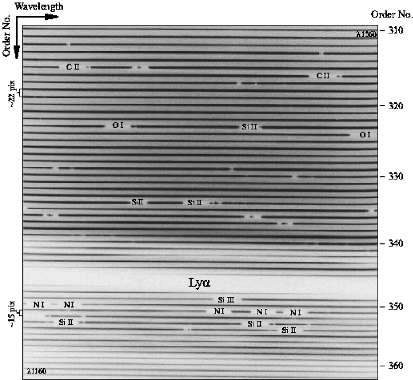
Figure 1: A view of a raw MAMA image taken with the STIS E140H grating and the $0\farcs 2\times 0\farcs 09$ aperture. Every tenth order is labelled, and we have identified several strong interstellar absorption lines. The target star is HD 218915, which lies behind gas associated with the Perseus spiral arm. In this figure, wavelength increases towards the right and towards the top of the page. The total wavelength coverage of this observation is approximately $1160-1360$ Å.

Figure 1 shows a raw two-dimensional STIS E140H FUV observation of the O9.5 Iab star HD 218915 covering the wavelength range $1160-1360$ Å. Several prominent interstellar absorption lines are labelled, and we have marked a number of spectral orders. The spectral orders at short wavelengths (bottom) are more tightly spaced than those at the long wavelengths (top). The usable spectral orders in this exposure run from 310 to 362 (with central wavelengths from $\sim 1358$ to 1162 Å, respectively). Some spectral regions occur in multiple orders. For example, two of the three lines in the N I triplet near 1200 Å appear in order 350 while the whole triplet is seen in order 351. Absorption due to C II $\lambda$1334 can also be seen in two spectral orders (315 and 316) in this image.

Figure 1 shows that the individual spectral orders are tilted with respect to the reference frame defined by the MAMA detector, and close inspection reveals they are slightly curved. In this paper we will be working with a product of the standard CALSTIS processing pipeline: two-dimensional geometrically-rectified images of each order. These flux- and wavelength-calibrated images have been extracted such that they are linear in both the wavelength and spatial (cross-dispersion) directions. The rectified images contain both the on-order spectral region as well as the adjacent inter-order light for each order.

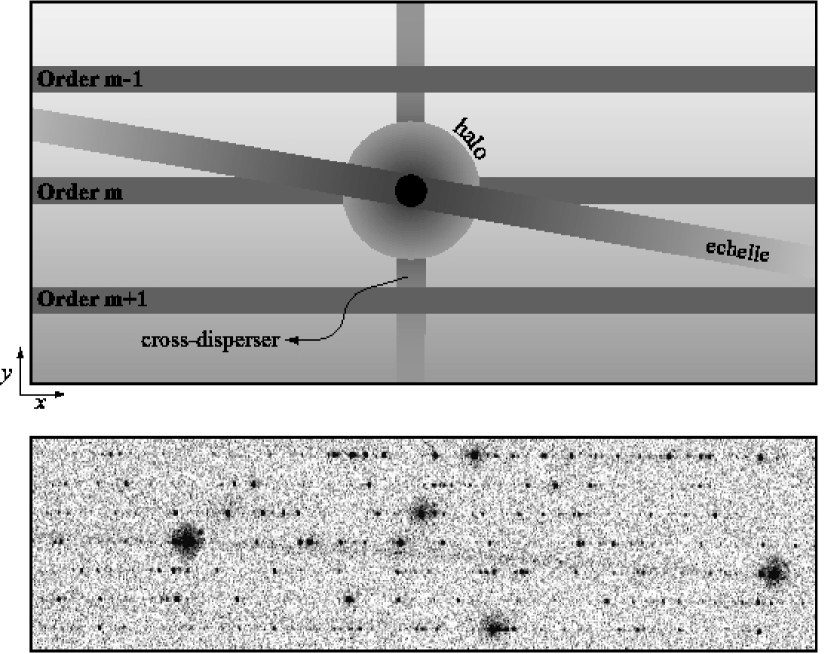
Figure 2: Top: A schematic showing the various possible scattering geometries for an emission line within the STIS two-dimensional echelle data. The rectified two-dimensional images discussed in the text include only one order and the inter-order light on either side of the order, although we have shown the adjacent orders in this figure. Of the three primary forms of background light illustrated, the most important are the effects of the detector halo and echelle scattering (see text). There is little evidence for a significant contribution from cross-disperser scattering (Landsman & Bowers 1997). The smaller-scale PSF halo is not illustrated in this figure. We only show the scattered light from the strong emission line in this figure; the true background will contain a contribution from the continuum as well. Bottom: A section of a deep post-flight STIS E230H wavelength calibration lamp image. This region is centered between 2400 and 2500 Å, and includes several orders. Wavelength increases to the right and towards the top of this image. (This section has been flipped across the horizontal axis to be consistent with the schematic and with Figure 1; E230H images typically have wavelengths increasing towards the bottom of the image.) A strong emission line occurs in both the third and fourth orders from the bottom of this image section. The strong halos can be seen surrounding both images of this particular line, while the faint signature of echelle scattering can also be discerned.

Figure 2 schematically illustrates the geometry of the two-dimensional rectified images (top panel). A portion of a STIS comparison lamp observation (taken with the E230H grating) is also shown (bottom panel). We define the $x$ and $y$ axes to follow the dispersion and cross-dispersion directions, respectively, in these images. The center of a spectral trace is defined to be at the position $y_{0}$, and the on-order light can be approximately described by a narrow Gaussian centered on this point. Though the rectified images we will be using contain only one order, we have shown several in Figure 2 for the sake of illustration.

Figure 2 also illustrates several potential forms of background light in the STIS echelle modes, and many of these can be identified in the accompanying comparison lamp image. We will discuss each of these sources of background light below. Sources of scattered and background light in the STIS echelle modes are also discussed briefly by Bowers et al. (1998) and Landsman & Bowers (1997). For comparison we point the reader to Cardelli et al. (1990, 1993) for discussions of the scattering geometry in the GHRS echelle modes, and to Schroeder (1987) for echelle geometry in general.

Both the echelle and cross-disperser gratings can give rise to scattered light within the spectrograph. Cross-disperser scattering will cause light from the order to be projected perpendicular to the spectral order, i.e., along the $y$ axis, into the inter-order region. Cross-disperser scattering is thought to be a relatively minor contributor in the STIS echelle modes (Bowers et al. 1998; Landsman & Bowers 1997).

Echelle scattering will cause light to be dispersed into the inter-order region at small angles to the order along lines of constant wavelength. For example, a bright emission line will appear to be connected to the same wavelength in adjacent orders by echelle scattered light in the inter-order region (see Figure 2). This form of scattering can be an important contributor to the background light in the STIS high-resolution echelle modes. It is difficult to account for without an a priori knowledge of the incoming spectrum. The iterative approach adopted by the STIS IDT should be able to account for this form of scattered light more accurately than our approach outlined in §3.

Another important source of background light in the STIS echelle mode data is the detector “halo,” whose width for the MAMA detectors can be of the same magnitude as the separation between orders (Landsman & Bowers 1997). The background spectrum caused by the detector halo will include contributions from the on-order spectrum of interest, $m$, and potentially light from the adjacent orders, $m\pm 1$, as well. Unlike light scattered by the cross-disperser and echelle gratings, the detector halo creates a background with an (approximately) axisymmetric pattern.

Similarly, the halo of the telescope point spread function (PSF) will be an additional source of background light. (This form of background light is not illustrated in Figure 2). This is essentially light from the wings of the PSF that arrives at the gratings with a slightly different angle than the narrow core of the PSF. Thus the halo creates its own, lower resolution version of the primary on-order spectrum that is also more extended in the spatial (cross-dispersion) direction.

Other potential sources of stray light in the STIS echelle modes include scattered light in the telescope assembly, large angle dust scattering, grating ghosts, reflections off of detector windows and other instrument components along the light path, and perhaps others. There is also a component of the background caused by particle radiation and phosphorescent emission from the detector window, which is particularly important for the NUV MAMA observations (Kimble et al. 1998).

3 Deriving the On-Order Background Spectrum

The background in STIS echelle observations is quite complex, with several sources of scattered and background light. Unfortunately, little information on the scattering properties of the instrument is available in the astronomical literature or through the various STIS instrument teams. We point the reader to the short discussion of the background and scattered light properties of the instrument by Bowers et al. (1998) and Landsman & Bowers (1997) for the best summaries provided by the STIS IDT.

The level of scattered light can vary significantly within an order, as judged by the residual flux levels in the saturated cores of strong interstellar absorption lines in gross (non-background corrected) spectra. Thus a common flux offset to the data at all wavelengths is insufficient as a background estimate. The appropriate zero levels of such saturated lines can vary by $\sim 10\%$ of the local gross continuum within a given order. Furthermore, the background level also varies significantly from order to order, making an average global correction inappropriate.

Given the complexities of the origins of the scattered and background light (and the instrument in general), we have developed an algorithm for estimating the on-order background spectrum that does not explicitly model the sources of background light. Instead, we empirically estimate the on-order background spectrum given the structure in the inter-order regions of the MAMA detector for each individual spectral order.

Similar empirically-derived approaches have been successfully applied for various other instruments using echelle gratings with two-dimensional detectors (e.g., Churchill & Allen 1995; Jenkins et al. 1996). Our method is different than those developed by Churchill & Allen (1995) for application to the Hamilton Echelle Spectrograph and by Jenkins et al. (1996) for the IMAPS instrument. In those cases the contribution to the on-order gross spectrum from the adjacent orders is derived using the known cross-dispersion profile of the closely-spaced spectral orders. The effects of order overlap are not as significant in the STIS echelle-mode observations as in either of these instruments. The background in our case is dominated by the broad halo surrounding an order, with much smaller contributions from the halos of the adjacent orders; echelle scattering can also be important (see §2).

3.1 The Method

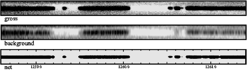
Figure 3: Sections of the two-dimensional rectified gross ($g_{i,j}$), background ($b_{i,j}$), and net ($n_{i,j}$) images for STIS E140H observations of the star HD 218915. These images cover the wavelength range 1258.6 to 1261.4 Å in order 334. A wavelength scale is given on the bottom net spectrum image. All images are shown on the same intensity scale, which is truncated at zero flux. In this example, the background image has not been smoothed before subtracting it from the gross image. The average residual flux in the inter-order regions of the net image is less than 0.09% of the average on-order flux and has a dispersion $\lesssim 0.3\%$ of the average on-order flux. A small amount of echelle scattering of the saturated interstellar lines into the inter-order background can be seen below the right-most portions and above the left-most portions of the gross image. The high-frequency noise observable in the background image is removed after extracting the one-dimensional background spectrum (see text).

In this section we present the procedure we have developed for deriving the on-order background for STIS E140H and E230H observations. Our approach is to fit the cross-dispersion profile of the observed inter-order light in a manner that correctly estimates the background at each position in the on-order spectrum. The steps used in our background removal procedure are as follows. (1) Produce two-dimensional rectified gross and error images of each order using CALSTIS. (2) Compress the image for a given order along the dispersion direction, thereby producing an average cross-dispersion profile. (3) Fit and subtract a rough background to the average cross-dispersion profile derived in step 2. (4) Identify the center of the spectral trace in the background-subtracted average cross-dispersion profile. (5) Identify the inter-order background regions in the gross image as those having less than 3.5% of the peak on-order flux. (6) Smooth the inter-order background with a two-dimensional Gaussian kernel. (7) Fit the cross-dispersion inter-order background profile at each wavelength with a seventh-order polynomial, weighting points nearer the spectral trace more heavily than more distant points. This step produces a two-dimensional background image after the background has been fit for each wavelength (e.g., Figure 3). (8) Extract one-dimensional gross, error, and background spectra from their respective two-dimensional images by summing over a seven-pixel extraction box centered on the spectral trace (summing in quadrature in the case of the error spectrum). (9) Smooth the background spectrum with a 17-pixel Lee (1986) local statistics filter. (10) Subtract the smoothed background spectrum from the gross spectrum to produce the final, net spectrum.

The process presented above is relatively simple. However, each of the steps has been optimized to give the best background fit, and therefore each requires a slightly more thorough discussion. We present the details of each of the steps of our technique below.

(1) For each order in the observation, we produce the geometrically-rectified two-dimensional gross and error images, which we denote $g_{i,j}$ and $e_{i,j}$, respectively, using the standard CALSTIS software available at the Space Telescope Science Institute. For our purposes, $i$ and $j$ refer to the dispersion and cross-dispersion direction, respectively. In this case, increasing values of $i$ imply increasing wavelengths, $\lambda$. These images have been flux and wavelength calibrated, though our method works just as well for count rate images.

(2) We compress the gross image of a given order along the dispersion direction, creating an order-averaged cross-dispersion profile, $a_{j}$:

$$a_{j}\equiv\sum_{i}g_{i,j}.$$ (1)

We use this average profile to determine the $y$-position of the center of the spectral trace, $y_{0}$, and to define the background regions of the rectified gross image.

(3) The array $a_{j}$ contains contributions from both the on-order spectrum and the on-order and inter-order backgrounds. To approximate the average background pedestal in the collapsed spectrum, we fit a fourth order polynomial to the cross-dispersion averaged profile, excluding the inner 40% of the array. The rectified images are slightly smaller than twice the separation between the order of interest and its neighbors in the raw MAMA image. (The inter-order separation in the raw MAMA image scales linearly with the central wavelength of the order.) For short wavelength observations, the fitting process described above excludes the central 12 pixels (the FWHM of the spectral trace is $\sim 2-3$ pixels). This rough fit is subtracted from $a_{j}$, producing a background-subtracted order-averaged cross-dispersion profile, $a_{j}^{0}$.

(4) We identify the $y$-position of the center of the spectral trace, $y_{0}$, with the maximum of $a_{j}^{0}$. Although a Gaussian fit may be more appropriate in theory, in practice we find identifying the center of the spectral trace by its maximum is sufficient.

(5) After identifying the center of the trace, we define the background regions, $y_{b}$, of the two-dimensional gross image to be those points where $a_{j}^{0}<0.035\,{\rm max}(a_{j}^{0})$. Those points that meet this criterion will be used in fitting the cross-dispersion profile of the inter-order background light. We have experimented with many different cut-off criteria for defining the background regions in the two-dimensional rectified images. The resulting background estimate can be somewhat sensitive to this parameter. Our experimentation suggests a cut-off at $3.5\%$ of the peak collapsed spectrum intensity is appropriate in most cases. The derived backgrounds are similar if one uses cut-off levels in the range $\sim 2\%-5\%$. The $y$-coordinates of the background regions are the same for each wavelength within an order.

(6) After determining which regions of the image $g_{i,j}$ make up the off-order background, we smooth those regions with a two-dimensional Gaussian having FWHM of 1.0 and 2.5 pixels in dispersion and cross-dispersion directions, respectively. This reduces some of the statistical noise, making the fitting process less susceptible to random noise fluctuations.

(7) Next we produce a background image, $b_{i,j}$, of the same dimension as the gross and error images by fitting a one-dimensional seventh-order polynomial to the cross-dispersion background profile at each point $i$ (each wavelength $\lambda$). Without the smoothing of the previous step, the background image produced, $b_{i,j}$, contains an excessive amount of small-scale structure. The importance of each cross-dispersion point, $y_{j}$, in the fitting process is weighted by $|y_{j}-y_{0}|^{-1/2}$, so that regions closest to the on-order spectrum are weighted more strongly than points at large distances from the spectral trace. Several different weighting schemes were tested, and the results were relatively insensitive to the weighting scheme for those weighting points toward the center more heavily. More uniform weighting schemes generally do not work as well. Only those points $y_{j}$ contained within $y_{b}$ are used in the fitting process.

We have found that fits using polynomials of higher order than seventh often give spurious results (particularly given the small number of background points used in the fits at short wavelengths). Lower-order fits often fail to adequately describe the curvature in the inter-order light distribution as well as the adopted seventh-order fits.

(8) After creating a background image, we extract one-dimensional gross, background, and error spectra using a seven-pixel extraction box. For the gross and background images, the seven points centered on the spectral trace are summed to produce the on-order gross spectrum ($g_{\lambda}$) and initial background spectrum ($b_{\lambda}^{\prime}$):

$$g_{\lambda}\equiv g_{i}=\sum_{j=y_{0}-3}^{y_{0}+3}g_{i,j},$$ (2)

and

$$b_{\lambda}^{\prime}\equiv b_{i}=\sum_{j=y_{0}-3}^{y_{0}+3}b_{i,j}.$$ (3)

The error spectrum, $e_{\lambda}$, is produced by adding the seven central pixels in quadrature:

$$e_{\lambda}\equiv e_{i}=\left(\sum_{j=y_{0}-3}^{y_{0}+3}e_{i,j}^{2}\right)^{1/2}.$$ (4)

We have chosen to adopt a seven-pixel summation extraction box to match the standard CALSTIS routines, though other extraction box sizes can be adopted. An optimal extraction routine may also be used.

(9) The final background spectrum, $b_{\lambda}$, is produced by smoothing the extracted background spectrum $b_{\lambda}^{\prime}$ with a 17-pixel Lee (1986) local statistics filter. The Lee filter effectively removes high-frequency noise in flat regions of the spectrum while leaving high-contrast edges in the spectrum intact. This is particularly important for spectra containing narrow interstellar absorption lines.

(10) The final net spectrum, $n_{\lambda}$, is the difference between the gross and smoothed background spectra, $n_{\lambda}\equiv g_{\lambda}-b_{\lambda}$.

3.2 Illustration of the Method

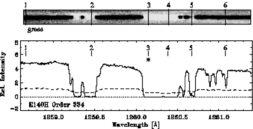
Figure 4: The final extracted net spectrum ($n_{\lambda}$; solid histogram) and background spectrum ($b_{\lambda}$; dashed line) for the spectral region in Figure 3 shown with the gross spectral image ($g_{i,j}$). Several positions in the spectrum are marked, and the cross-dispersion profiles at these positions are shown in Figure 5. The background at position 3 is slightly over-estimated, leaving a negative residual flux in the short wavelength portion of the saturated Si II absorption.

Figure 3 shows a portion of the raw, two-dimensional rectified gross image ($g_{i,j}$) of order 334 taken from the E140H observation shown in Figure 1. Also shown is the corresponding two-dimensional background image ($b_{i,j}$) derived as described above, and the difference of these images ($n_{i,j}\equiv g_{i,j}-b_{i,j}$). All of the images shown in Figure 3 are displayed with the same intensity scale, which is truncated at a low level to show the structure of the inter-order background. The wavelength coverage of this section of the spectrum is $\lambda\approx 1258.6$ to $1261.4$ Å; this region includes absorption from S II $\lambda$1259 and Si II $\lambda$1260 (as well as weaker absorption from Fe II $\lambda$1260 and C I $\lambda$1261). The final extracted net spectrum ($n_{\lambda}$) and background ($b_{\lambda}$) are shown in Figure 4.

Several aspects of Figure 3 are noteworthy. First, the echelle scattered images of the saturated interstellar absorption lines are vaguely visible in the inter-order regions of the $g_{i,j}$ image. These can also be seen to some extent in the model background image, $b_{i,j}$. The background image contains the imprint of echelle-scattered light since the fitting process does not specifically exclude such regions. Second, the background image, $b_{i,j}$, shows significant high-frequency variations in the dispersion direction. This is a result of fitting each column (wavelength) independently. The application of the Lee filter to the extracted one-dimensional background spectrum, $b_{\lambda}^{\prime}$, removes much of this high-frequency noise from the final background spectrum, $b_{\lambda}$ (see §3.1). The inter-order regions of the background-subtracted image, $n_{i,j}$, are relatively smooth and very near zero residual intensity. There is little residual large-scale structure in the background regions of the $n_{i,j}$ image.

Figure 5 shows several examples of cross-dispersion profiles (histogram) extracted from the rectified two-dimensional image of this order. The cross-dispersion profiles are numbered, and the positions of these profiles in wavelength space are marked on the image and spectrum shown in Figure 4. These profiles are drawn from several different regions of the spectrum, including continuum regions (position 1) as well as regions that include weak (positions 5 and 6) and strong (positions 2 through 4) absorption. The smooth curves plotted on top of the cross-dispersion profiles show our one-dimensional polynomial fits to the inter-order background, and the squares mark the data points used for deriving those fits. One can see that the inter-order backgrounds are well fit at most of these positions. A counter-example is position 3, which is marked with a star in the spectrum shown in Figure 4. In this case the background is over-estimated. The difficulty in fitting this position is caused by the effects of echelle scattering; we will discuss this in more detail in §4.

To show how the background we are fitting in these cross-dispersion profiles relates to the larger-scale distribution of light in the two-dimensional MAMA images, we present a cross-dispersion profile through several orders in Figure 6. The distribution shown here is drawn from the raw (gross) MAMA observation of HD 218915. The identifications of the orders are given along the top of the figure. This particular cross-dispersion cut passes through the saturated troughs of two strong interstellar lines: N I $\lambda$1200.2 in order 351 and Si II $\lambda$1193.3 in order 353. Figure 6 shows a background fit for order 351 as the solid line. The points used in this background fit are marked with filled squares, as in Figure 5.

One can see that while the orders are closely spaced, the excellent image quality of HST concentrates the on-order light into the central few pixels. Thus it is only the wings of the halos from adjacent orders that overlap and not the cores of the on-order light distribution. This can be compared with the cross-dispersion profiles shown in Churchill & Allen (1995) and Jenkins et al. (1996), where the overlap of light from adjacent orders is much more significant.

3.3 Potential Limitations

The procedure we have outlined above is quite simple and can be summarized as a single step: we fit the cross-dispersion profile of the inter-order light to estimate the on-order background spectrum. It seems established, however, that the cross-disperser gratings provide little to the scattered light budget of the STIS echelle modes (Bowers et al. 1998; Landsman & Bowers 1997). The more important causes of scattered and background light in the echelle modes are the PSF halo, the detector halo, echelle grating scattered light, and the particle/phosphorescent background. Neither the halos nor the echelle scattering give a pure cross-dispersion profile of scattered light. It is important to consider the effects this may have on the approach outlined in §3.1, given that we are only fitting the cross-dispersion profile of the background light.

The PSF and detector halos provide (roughly) axisymmetric scattering about a given point in the spectral trace (see lamp spectrum in Figure 2). Thus, this type of scattering distributes light both in the dispersion and cross-dispersion directions. The inter-order light at a given point contains halo-scattered light that originates from several different wavelengths. The weighting of data points close to the spectral trace in our inter-order background fits causes light scattered at small angles from the dispersion direction by the PSF and detector halos to play an important role in the resulting estimate of the on-order background spectrum.

The broad halos surrounding an order seem to be the dominant source of on-order background. For continuum sources the effects of the halos of orders $m\pm 1$ are significantly less than the halo of the order $m$. To quantify this we have derived a composite cross-dispersion profile showing the distribution of halo light as a function of distance from an order. Figure 7 shows composite cross-dispersion profiles derived for two wavelength regions. The top plot shows a region near 1216 Å derived from E140H observations of strong Ly$\alpha$ emission the solar analog $\alpha$ Centauri A (kindly made available to us by J. Valenti). The bottom plot shows a region near 2800 Å derived from Mg II emission from $\alpha$ Orionis. The intensities have been normalized to unity at the center of each order. The points are averages of emission from two orders (346 and 347 for the E140H data and 276 and 277 for the E230H data) drawn from the brightest emission regions in these spectra. We have averaged only one side of each order to exclude the brightest echelle-scattered light. The filled circles have intensities $\leq 3.5\%$ of the peak and would hence be used in constructing the background using our procedure (see §3.1). The bump of excess emission centered at $|\Delta y|=18$ (marked as $m\pm 1$) in the E140H plot is caused by weak emission from the adjacent orders. The adjacent orders in the E230H plot are located at $|\Delta y|=37$, i.e., beyond the edge of the plot.

At the position of the adjacent order for the E140H data ($|\Delta y|=18$ in Figure 7), the expected relative intensity of the broad halo from the central order is only a few percent of its peak (extrapolating the halo contribution marked with filled circles to $|\Delta y|=0$). The contribution from the halos of adjacent orders to the order being extracted is therefore expected to be only a few tenths of a percent of the peak on-order flux. Similar limits can be derived from the lack of strong spectral features from adjacent orders $m\pm 1$ in the gross spectrum of an order $m$. The contribution of the halos from orders $m\pm 2$ to an order $m$ should be less than 0.1% of the contribution of its own halo. For the E230H distribution, the halos have a flatter decline with distance from the center of the order. However, the overall level of the halo is significantly lower relative to the peak intensity in the center of the order compared with the E140H distribution. This is consistent with the much lower level of the backgrounds seen at 2800 Å than at Ly$\alpha$ (see §4.3).

For continuum regions the halo contribution from the current order is much more important than that from the adjacent orders. This is in part why we have not adopted a method similar to that of Churchill & Allen (1995) or Jenkins et al. (1996). In cases where strong emission lines are present in an adjacent order, it is true that the contribution from the halo of an adjacent order $m\pm 1$ can be more important than the local halo if the emission from the local order $m$ is very weak.

Light scattered by the echelle gratings is the single most important limiting factor in our approach. In theory, if the spectrum scattered into the inter-order region is smooth over relatively large scales, echelle-scattered light could be accurately fit by our technique. In that case, the inter-order light is a smoothly varying function in the cross-dispersion direction, i.e., there is a degeneracy between cross-disperser and echelle scattering in the inter-order regions for a smooth spectral source. However, there are small-scale structures in the scattered spectrum (e.g., interstellar absorption features, particularly the strongly saturated lines). In the case where strong or numerous small-scale spectral features are scattered by the echelle gratings into the inter-order regions, the validity of our approach may break down. Echelle scattering of local interstellar features into the inter-order regions can bias the cross-dispersion fits (see §4). This will be particularly true if the scattering by the echelle gratings makes up a very large fraction of the scattered light budget.

In general, we believe the relative echelle scattering contribution to the total on-order background spectrum is less important than the detector halo (in terms of the relative intensities). Using the E230H lamp observation shown in Figure 2, we estimate that the echelle scattering contribution to the interorder background at $\lambda\sim 2450$ Å is $<5\%$ of the contribution from the halo seen surrounding strong emission lines. Using the aforementioned E140H observations of Ly$\alpha$ emission from $\alpha$ Cen, we have found that the peak intensity of the echelle-scattered emission is equivalent to the strength of the halo shown in Figure 7 at $|\Delta y|\approx 10$ pixels (i.e., $\lesssim 10\%$ of the expected halo intensity near the center of the order).

However, the impact of echelle scattering on our method is more important than its intensity relative to the broad detector halo would suggest. Discrete features in the echelle-scattered inter-order light adversely effect the cross-dispersion fits in some cases. Thus the results for regions near very strong, sharp absorption (or emission) lines will need to be viewed with caution, particularly at short wavelengths where the inter-order separation is smaller. This is discussed more fully in §4.

4 Results

4.1 Examples and Uncertainties

In this section we show several examples of STIS high-resolution echelle data extracted as discussed in §3. The wavelength regions shown contain strongly-saturated interstellar lines. These flat-bottomed lines, which should have zero residual flux, offer a chance to assess the quality of the background subtraction through their shape and flux level. A detailed comparison of STIS data extracted with our algorithm and archival GHRS data will be given in §5. We draw examples in this section both from archival STIS data and our own guest observer program (STScI program #7270).

Figures 8, 9, and 10 show examples of short wavelength ($\lambda<1350$ Å) E140H spectra for the stars HD 218915, HD 185418, and HD 303308, respectively. The four spectral regions shown in these figures contain saturated absorption lines near 1200 Å (the N I triplet), 1260 Å (S II $\lambda$1259 and Si II $\lambda$1260), 1302 Å (O I $\lambda$1302 and Si II $\lambda$1304), and 1334 Å (C II $\lambda$1334 and C II^∗ $\lambda$1335). The solid lines show the background-corrected on-order spectrum, $n_{\lambda}$, while the dashed lines show the on-order background spectrum, $b_{\lambda}$, that was subtracted from the extracted gross spectrum. For the region near C II $\lambda$1334, we have co-added two spectral orders (315 and 316) weighted by their respective error spectra.

Figure 11 shows several longer-wavelength spectra of HD 303308, including three spectral regions observed with the E230H grating. This figure shows four spectral regions that include the saturated absorption lines Al II $\lambda$1670, Fe II $\lambda$2382 and $\lambda$2600, and Mg II $\lambda$2796. As in the previous figures, the on-order background spectrum is shown as the dashed line.

The representative spectra shown in Figures 8–11 exhibit several common features of our data extraction routine. First, we find that the ratio of the on-order background spectrum to the on-order net (or gross) spectrum is higher in the shorter wavelength observations. This is consistent with expectation, particularly given the smaller order spacing at shorter wavelengths. The ratio of on-order background to gross spectrum will be discussed in more detail in §4.3.

Next, it is clear from Figures 8 through 11 that the quality of the background subtraction is much better at longer than at shorter wavelengths. For all the stars shown in these figures, the absorption due to C II $\lambda$1334 is flat-bottomed at zero flux level. Towards progressively shorter wavelengths, the saturated absorption profiles tend to show excursions from true zero with slight artifacts appearing in the black troughs. Figure 12 shows expanded views of regions of the HD 218915 spectra containing strongly-saturated interstellar absorption. The profile of Si II $\lambda$1260 in Figure 12 shows a slight over-subtraction of the background on the lower-wavelength end of the otherwise black absorption trough. The N I $\lambda$1199 profile seen in Figure 12 shows over-subtracted regions at various points along the absorption trough. The background in this case shows significant spurious structure (e.g., near $\lambda=1199.35$ Å). Over-subtraction of the background is seen for all three members of the N I triplet near 1200 Å (see Figure 8). However, C II $\lambda$1334 shows only a very small over-subtraction of the background. The long wavelength observations of HD 303308 shown in Figure 11 show no such artifacts, and the saturated absorption profiles are at the correct zero level over their entire breadth.

This characteristic over-subtraction of the background in short wavelength observations seems to be caused by the influence of echelle scattering of strong lines into the inter-order background on our cross-dispersion polynomial fits (see 3.3). Figure 5 shows several examples of cross-dispersion profiles extracted from the rectified two-dimensional image of order 334 in our E140H observations of HD 218915, as discussed in §3.2. Most of the cross-dispersion profiles shown in Figure 5 are examples of regions where our fitting procedure works well. Position 3, marked with a star in the spectrum shown in Figure 4, shows a wavelength region where our background fit overestimates the true background level. In this case, the saturated line core is over-subtracted by $\sim 1\%$ of the local continuum. The cross-dispersion profile for position 3 contains two regions, marked with open squares in Figure 5, with lower intensity than their surroundings (the order is centered at $y=15$). These discrete regions on either side of the spectrum are images of strong interstellar absorption from the on-order spectrum that have been scattered into the inter-order region by the echelle grating.

The dashed line over-plotted on the cross-dispersion profile of position 3 shows a polynomial derived by excluding these four points from the fit. The fit shown by the dashed line is significantly better than that used in deriving the spectrum shown near the bottom of the figure. However, we do not at present have an algorithm to identify and exclude such points from the cross-dispersion fits. If the spatial distribution of the echelle-scattered background were derived, and the effects of this scattering removed from the two-dimensional images before the cross-dispersion fitting described here, our approach would likely have fewer problems at short wavelengths. The method developed by Churchill & Allen (1995) for use with the Hamilton Echelle Spectrograph does in effect build a model two-dimensional background surface which is subtracted from the raw data before standard spectra-extraction techniques are applied. The derivation of the echelle scattering properties is, however, beyond the scope of this work.

Our emphasis in presenting (and testing) our background subtraction routines has been on observations of early-type stars, since these are the most important for studying the interstellar medium. However, our reduction techniques should also be suitable for most other types of observations. To demonstrate the applicability of our approach to other types of observations, we have reduced archival STIS E230H observations of $\alpha$ Orionis (Betelgeuse). The region surrounding the Mg II $\lambda$2800 doublet is shown in Figure 13. The saturated interstellar absorption lines seen on top of the stellar emission lines are flat bottomed at zero flux, as expected. We have also tested our routine on the aforementioned FUV STIS observations of the solar analog $\alpha$ Cen. In general our routines did an excellent job deriving the background for this emission line dataset. However, in the orders adjacent to the extremely bright Ly$\alpha$ emission from this star, the wings of the detector halo extended well into the very weak emission from the adjacent orders (see Figure 7). This caused our routines to over-subtract the very bright background from the very weak continuum and line emission in the orders adjacent to Ly$\alpha$. This is the one instance we have identified where our procedures are not able to appropriately fit the interorder background. Our tests suggest that, with this one exception, our extraction procedures are doing reasonably well even for late-type stars.

4.2 Caveats

Given the difficulties in fitting the cross-dispersion profiles at short wavelengths, where the halos of the closely-packed spectral orders may overlap significantly and the echelle scattering affects a greater fraction of inter-order pixels, we believe particular attention should be paid to background uncertainties. Lines having residual fluxes less than $10-20\%$ of the local continuum flux should be treated with care. Astronomers working with such lines in high-resolution STIS data should consider the effects of zero-point uncertainties that depend on wavelength in deriving column densities and other parameters. The fluctuations in our background estimates can be used to approximate the uncertainties in the overall zero level for individual spectral regions. For example, the standard deviation about the mean of the background spectrum in the spectral region encompassing the saturated Si II 1260 Å line is $\sim 0.6\%$ of the local continuum. The $2-3\,\sigma$ fluctuations are a good estimate of the potential error in the background spectrum in this case (as judged by the maximum oversubtraction of the Si II line). For lines with residual fluxes that are 10% of the local continuum, this implies potential systematic errors in the optical depth of order 10%.

Although the background subtraction at short wavelengths, e.g., $\lambda\lesssim 1300$ Å, often shows evidence of slight artifacts in the saturated absorption troughs of deep lines, we find little evidence for such problems in the longer wavelength observations. This is due to the larger order separation, generally higher signal-to-noise ratios, and smaller contribution of the on-order background to the gross spectrum. Data taken with the E140H grating at wavelengths in excess of $\lambda\gtrsim 1600$ Å and with the E230H grating at wavelengths $\lambda\gtrsim 2200$ Å (where $b_{\lambda}/g_{\lambda}\lesssim 0.1$; see §4.3) are likely more secure than shorter wavelength data in each of the gratings. And while we correctly state that these artifacts are present for wavelengths shorter than 1300 Å, the difficulties are most apparent wavelengths shortward of Ly$\alpha$. However, analysis of detailed line shapes for strong absorption should still be approached with caution for $\lambda\lesssim 1300$.

In general astronomers using a routine like the one outlined here may decide to apply a second-order correction that adjusts the output spectrum by a simple vertical flux offset. Such a shift is designed to bring the majority of a saturated line profile to the correct zero level in a given order. We have calculated the shift required to make the average of the saturated line profiles of the short wavelength lines observed towards HD 303308 equal zero flux. We find an offset of $1-2\%$ of the local continuum is most appropriate. Although we are skeptical that this is the best way to correct spectra where the saturated lines fall somewhat below zero, the correction is typically modest.

The quality of the background estimation using the algorithm presented here is dependent on the signal-to-noise ratio of the dataset. In low signal-to-noise ratio data, the polynomial fitting routine used in our method can produce spurious background excursions. Thus, if one wants to accurately remove the on-order background using our procedures, it is important to design observing programs that produce enough inter-order light to be accurately fit. For practical purposes, this means producing datasets with signal-to-noise ratios in excess of 20 is important for accurate background determinations.

4.3 The On-Order Background Fraction

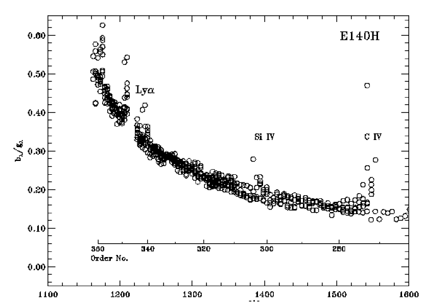
Figure 14: The fractional contribution of the on-order background light, $b_{\lambda}$, to the gross spectrum, $g_{\lambda}$ for several E140H observations of early type stars. Each point represents the median value of $b_{\lambda}/g_{\lambda}$ for an individual order of a particular observation. Data are presented for nine sightlines taken from the STIS archive or our own GO program; several sightlines were observed in multiple wavelength regions. Average and median $b_{\lambda}/g_{\lambda}$ values for specific orders are given in Table 1. Data taken through both the $0\farcs 2\times 0\farcs 09$ and $0\farcs 2\times 0\farcs 2$ apertures are shown. The dispersion at certain wavelengths is very large due to the presence of strong P Cygni-like stellar wind profiles in several of the stars (e.g., near C IV $\lambda 1550$) or strong interstellar absorption (e.g., near Ly$\alpha$). We have marked several such regions in this figure. We have excluded orders that are dominated by interstellar Ly$\alpha$ absorption. The ratio $b_{\lambda}/g_{\lambda}$ decreases approximately as $\lambda^{-3}$. These data were derived using observations of early-type stars. The $b_{\lambda}/g_{\lambda}$ ratio could depend on the spectral type.

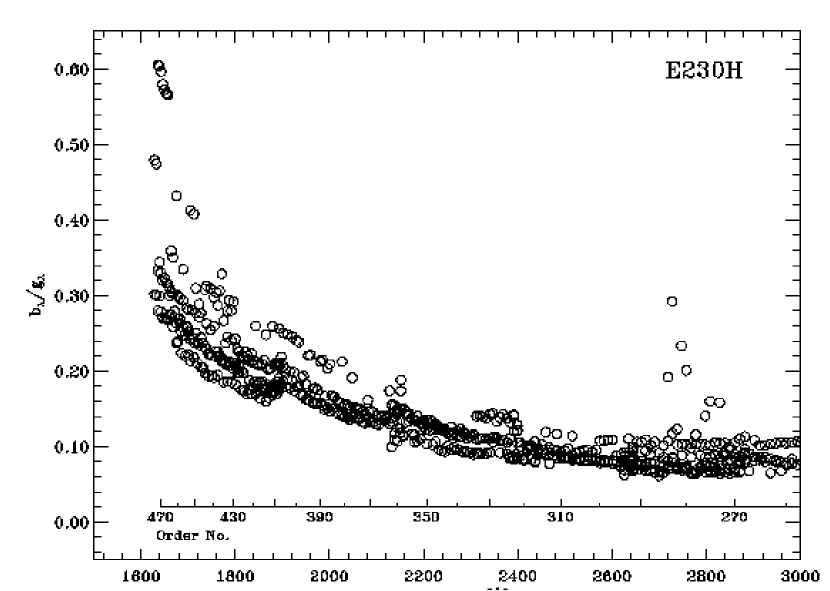
Figure 15: As Figure 14, but for data taken with the E230H grating. Data taken from 11 early-type stars, some of which are observed in multiple wavelength regions, are shown. The ratio $b_{\lambda}/g_{\lambda}$ again decreases approximately as $\lambda^{-3}$. Average and median $b_{\lambda}/g_{\lambda}$ values for specific orders are given in Table 2.

We have calculated the fractional contribution of the on-order background light to the on-order gross spectrum as a function of wavelength (spectral order) for a number of archival STIS datasets as well as our own guest observer program data. Figure 14 shows this fraction for the E140H grating. Each data point represents the median value of the extracted gross spectrum divided by the derived on-order background for a given spectral order within a single observation, i.e., the median of $b_{\lambda}/g_{\lambda}$. In making this plot, we have extracted the data in counts rather than flux. This removes any differences between the datasets caused by discrepant flux calibrations. Average and median values of the background to gross ratio are collected in Table 1 for several spectral orders. In Figure 15 and Table 2 we collect analogous values for data taken with the E230H grating. All of the stars included in these determinations are early type stars (O and B type, as well as one white dwarf). The ratio $b_{\lambda}/g_{\lambda}$ is likely to depend on the shape of the underlying stellar continuum. This is obvious even in the current data given the large dispersion that appears near strong P Cygni stellar wind lines (e.g., Si IV $\lambda$1400 and C IV $\lambda$1550 in Figure 14).

Figures 14 and 15 show a general decrease in the prevalence of the background light at longer wavelengths. This is in qualitative agreement with expectation, since most scattering phenomena show a decreasing intensity with increasing wavelength. For example, diffracted intensity decreases as $\lambda^{-2}$, while Rayleigh scattering intensity decreases as $\lambda^{-4}$. Furthermore, the order spacing increases with wavelength, making the fitting process more robust. We find that the background to gross fraction, $b_{\lambda}/g_{\lambda}$, decreases approximately as $\lambda^{-3}$ for both gratings. This scaling is relationship is only approximate, and the E140H data are not well fit by $b_{\lambda}/g_{\lambda}\propto\lambda^{-3}$ over the entire wavelength range tested. There is an excess in the $b_{\lambda}/g_{\lambda}$ at short wavelengths compared with this scaling, and the effects of strong stellar wind and interstellar absorption features are visible in many other wavelength regions (see Figure 14). Furthermore, the ratio $b_{\lambda}/g_{\lambda}$ for E230H data may rise beyond 3000 Å, though our data in that region are sparse.

The inter-order separation, $\Delta y_{m}$, in STIS high resolution echelle-mode observations increases linearly with wavelength. Hence the background to gross fraction, $b_{\lambda}/g_{\lambda}$ can be described as cubic polynomial of $1/\Delta y_{m}$. Again, this scaling is not perfect for E140H data. Churchill & Allen (1995) have shown a similar correlation between the order separation and (in their case) inter-order intensity, and they have used it to argue that the contamination of adjacent orders $m\pm 1$ (and beyond) was the most important determiner of the on-order background spectrum in data from the Hamilton Echelle Spectrograph. However, we do not believe that order overlap effects are causing the relationship seen in Figures 14 and 15. The lack of direct order overlap and the relatively small contribution from the halos of adjacent orders (see Figure 7) in the STIS data strongly suggests neither of these is driving the relationship seen in Figures 14 and 15. Potentially more likely is the effect of echelle scattering for small order separations, but our discussion in §3.3 suggests this contribution may not be enough to cause these relationships either. It is more likely that Figures 14 and 15 are tracing the wavelength dependence of the processes causing the scattered and background light.

The background to gross fractions shown in Figures 14 and 15 are dependent on the size of the extraction box used in determining the gross and background spectra. The cross-dispersion profile of the spectral trace is roughly Gaussian (see Figure 5). Our default extraction procedure adopts a seven pixel extraction box (from $y_{0}-3$ to $y_{0}+3$, where $y_{0}$ is the center of the spectral trace). The outer-most pixels in the extraction box have much higher background to gross values than the inner-most pixels. Thus, if only the central three pixels were used in the spectral extraction (e.g., $y_{0}-1$ to $y_{0}+1$), the on-order background to gross ratio would be significantly lower. Experiments using a three pixel extraction box for data near 1250 Å suggests the decrease in $b_{\lambda}/g_{\lambda}$ can be of order 30%.

Given the relatively large contribution of the on-order background light to the gross spectrum at short wavelengths, it may be better in some cases to use smaller extraction boxes. The size of the extraction box can be chosen to minimize the impact of statistical noise in the background on the extracted net spectrum. If the shortest wavelength region is vital to a STIS program, the background fraction must be accounted for when calculating exposure times.

5 Comparisons with GHRS Data

In order to assess the accuracy of our STIS background correction scheme, we will compare STIS data extracted as described above with data from the previous high-resolution UV spectrograph on-board HST, the Goddard High Resolution Spectrograph (GHRS). This section presents two such comparison datasets. First, we compare STIS E140H observations of HD 218915 with observations of the same star made with the first-order G160M grating of the GHRS. The scattered light properties of the intermediate resolution G160M grating are excellent (see Cardelli et al. 1993), making data obtained with this grating a good point of comparison for our background correction. Second, we compare archival STIS E140H observations of the nearby DA white dwarf G191-B2B with GHRS Ech-A high-resolution data for the same star. The resolutions of the STIS and GHRS G191-B2B datasets are similar, allowing a good comparison without the need to smooth the STIS data.

5.1 Comparison of STIS E140H and GHRS G160M Observations of HD 218915

The star HD 218915 lies behind gas associated with the Perseus arm; it was observed extensively with the GHRS first-order G160M grating. We have retrieved these data from the HST archive and reduced them as described by Howk, Savage, & Fabian (1999). These data, taken through the small science aperture ($0\farcs 25\times 0\farcs 25$) before the installation of COSTAR, have a velocity resolution of $\sim 18.6$ km s^-1 (FWHM) at 1250 Å. Our comparison of the STIS and GHRS data for this sightline will focus on the S II lines $\lambda 1250$, 1253, and 1259 and Si II $\lambda 1260$; strong C I absorption is also seen in this spectral region (see Figure 8).

The STIS E140H data, which have a resolution $\Delta v\sim 2.75$ km s^-1, must be smoothed for a direct comparison with the intermediate-resolution GHRS G160M data. We have convolved the higher-resolution STIS data, after combining several spectral orders, with a Gaussian having a FWHM of 18.4 km s^-1 and rebinned these smoothed STIS data to approximately the same sampling as the GHRS data. We have also normalized the STIS data with a linear continuum to bring the slope and continuum intensity levels of the GHRS and STIS data into agreement. After the standard background subtraction, we find no evidence for residual scattered light in the GHRS G160M observations, as judged by the saturated core of Si II $\lambda 1260$.

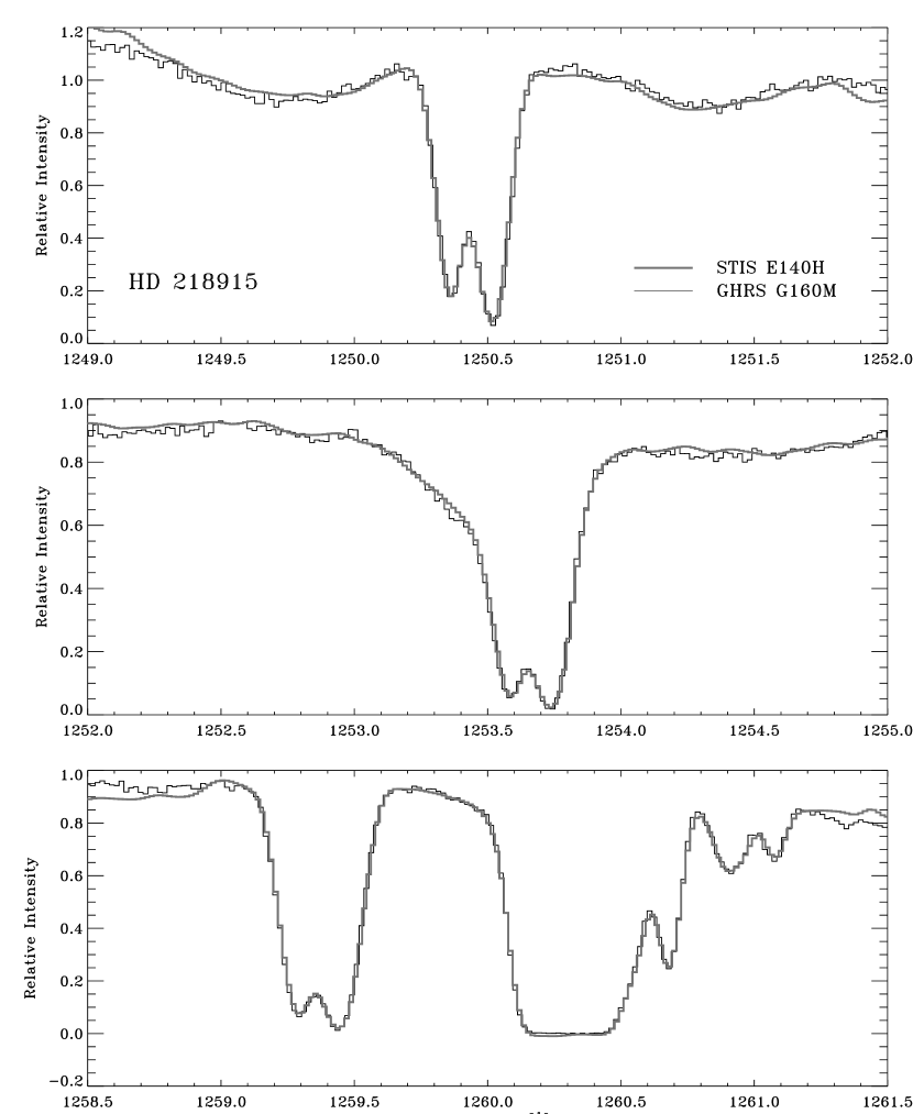
Figure 16: A comparison of STIS E140H and GHRS G160M observations of the star HD 218915 in three spectral regions containing S II, Si II, and C I interstellar absorption. The STIS data, displayed as a thick grey line, have been smoothed and rebinned to the effective resolution of the GHRS data ($\sim 18.6$ km s^-1). A rough linear continuum has been removed from the STIS data, and both datasets have been arbitrarily scaled by a multiplicative constant to best match one another. The agreement between these two sets of observations is excellent at most wavelengths. A slight over-subtraction of the STIS data in the core of Si II $\lambda 1260$ is visible. The agreement between the two datasets is particularly encouraging given the good scattered light properties of the GHRS G160M grating. The smoothed versions can be compared with the full-resolution STIS observations shown in Figure 8.

Figure 16 shows the comparison between the GHRS G160M data and the smoothed STIS E140H data extracted with our background correction scheme. The top panel shows absorption due to S II $\lambda 1250$, the middle panel shows S II $\lambda 1254$, and the bottom panel includes absorption from S II $\lambda 1259$, Si II $\lambda 1260$ (blended with Fe II), and several lines of C I. Unsmoothed data for the spectral region covered in the bottom panel are shown in Figure 8. We have removed a slight velocity offset between the two datasets in producing Figure 16.

The agreement between the two datasets shown in Figure 16 is generally excellent. The depths and shapes of all three S II lines are in good agreement between the STIS and GHRS datasets. The STIS Si II $\lambda$1260 profile exhibits the slight oversubtraction of the saturated line core that we have pointed out previously (on the low wavelength end). However, the rest of the Si II profile and the adjoining C I transitions show remarkable agreement in the two datasets. We find a similar agreement between the longer wavelength transitions of Si II $\lambda$1526 and C IV $\lambda$1548, though we do not show those data.

Given the good scattered light properties of the first-order GHRS G160M grating, the agreement between these two datasets suggests our background subtraction algorithm is producing reliable estimates of the on-order background spectrum, within the limits of this comparison. The heavy smoothing required to compare the STIS and GHRS datasets could potentially mask important differences in the datasets.

5.2 Comparison of STIS E140H and GHRS Ech-A Observations of G191-B2B

The nearby ($d\sim 69$ pc) DA white dwarf G191-B2B has been well-observed by both the STIS and GHRS in their high-resolution modes. The low column density of material along this sightline [$\log N(\mbox{{H~{}I}})\sim 18$ in atoms cm^-2] has made it important for studying the D/H abundance in the local ISM. Results derived from the GHRS observations have been published by Vidal-Madjar et al. (1998). The STIS data have been published by Sahu et al. (1999), who used the STIS IDT background correction algorithm (Bowers & Lindler, in prep.) in their data reduction.

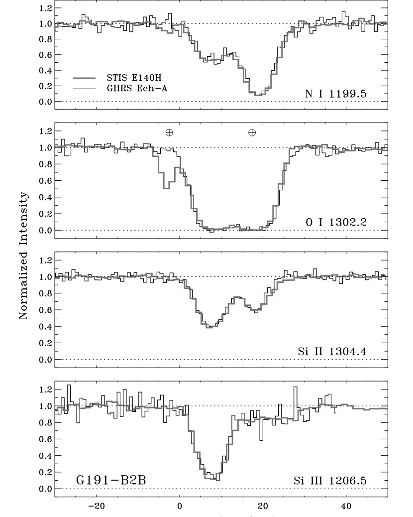
Figure 18: A comparison of archival STIS E140H and GHRS Ech-A observations of interstellar absorption lines towards the DA white dwarf G191-B2B. We show normalized absorption line profiles as a function of velocity for the ions N I, O I, Si II, and Si III. The STIS data are shown as a thick grey line. We have marked the positions of telluric absorption lines in the O I profile ($v\sim-2.5$ km s^-1 for the STIS observations and $v\sim 17.4$ km s^-1 for the GHRS observations). The GHRS Si III observations are at the end of the detector diode array, making the continuum placement uncertain. In general we find excellent agreement between these two datasets.

We retrieved the archival GHRS Ech-A data for G191-B2B and reduced them as described by Howk et al. (1999). There are a large number of GHRS exposures covering the region of the spectrum containing interstellar Ly$\alpha$. We summed all those exposures taken at the same grating carrousel position within an individual observation (visit). We then merged the resulting vectors using the standard wavelength scales, at the same time solving for and removing the fixed-pattern noise spectrum. The standard GHRS background subtraction over-estimates the background level near the saturated interstellar Ly$\alpha$ profile. We adopted a value for the “$d$-coefficient” of $d=0.002$ to bring this saturate profile to the appropriate zero-level (see Cardelli et al. 1990, 1993). All of the other data presented here have been reduced using the standard $d$ values of Cardelli et al. (1993). The G191-B2B GHRS data presented here were all taken through the small science aperture. The Si III profile lies at the edge of the Digicon detector array in the GHRS observations of the 1206 Å region. We have used only the three (of four) FP-SPLIT positions where the Si III absorption was shifted away from the edge of the detector array in deriving the profile seen in the bottom panel of Figure 18.

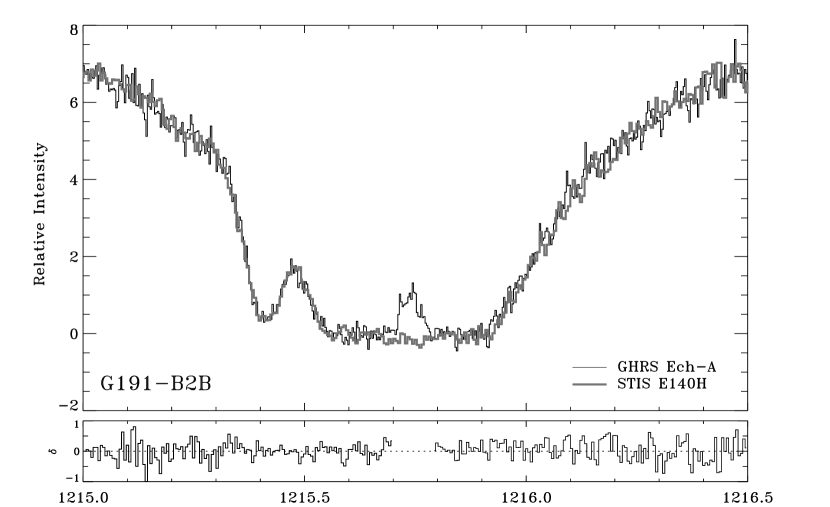
Figure 17: A comparison of the interstellar H I and D I Lyman-$\alpha$ observations towards the DA white dwarf G191-B2B using STIS and GHRS. This figure can be directly compared with Figure 3 of Sahu et al. (1999). The post-COSTAR GHRS data have slightly lower resolution but higher sampling. Our extractions of the STIS data are shown by the thick grey line. We have coadded two orders (346 and 347) in our STIS extraction. The bottom panel shows the difference between the GHRS data (after rebinning to the same sampling as the STIS data) and the STIS data. The GHRS data include airglow emission in the center of the Ly$\alpha$ profile that is not present in the STIS data; the residuals from the region containing this emission are not shown. The residuals between the two datasets are completely consistent with the formal STIS errors (71% of the residual points fall within $1\sigma$, while 95% of the residual points fall within $2\sigma$). There is no compelling reason to believe that the STIS and GHRS data along this sightline are in disagreement as suggested by Sahu et al. (1999). Our GHRS Ly$\alpha$ profile is in good agreement with that of Vidal-Madjar et al. (1998).

Figure 17 shows a comparison of our extraction of the STIS E140H observations of the wavelength region surrounding Ly$\alpha$ with the GHRS Ech-A observations of this line. We have co-added two overlapping orders to produce the STIS profiles (orders 346 and 347). The GHRS data have been scaled by a multiplicative constant to match the STIS data. The velocity resolution of the GHRS Ech-A data ($\sim 3.5$ km s^-1) is somewhat worse than the resolution of the STIS E140H data; however, the GHRS data have finer sampling ($\sim 0.88$ km s^-1 vs. $\sim 1.25$ km s^-1 for the STIS E140H data). Figure 3 of Sahu et al. (1999) compares the STIS Ly$\alpha$ profile as extracted with the IDT reduction routines with their reduction of the GHRS Ech-A data (though they have applied a three-pixel smoothing kernel to their data).

Again, the agreement between the GHRS and STIS profiles shown here is excellent. The curves are virtually indistinguishable, save for the geocoronal Ly$\alpha$ emission in the center of the GHRS profile. The center of the STIS Ly$\alpha$ profile shows a slight over-subtraction, consistent with the discussion in §4. The D I Ly$\alpha$ profiles are in excellent agreement. There is no compelling reason to believe that the STIS and GHRS data along this sightline are in disagreement as suggested by Sahu et al. (1999). Our GHRS Ly$\alpha$ profile is in good agreement with that of Vidal-Madjar et al. (1998). Our profile is in agreement with that derived by the IDT reduction software to within the statistical and background uncertainties.

Figure 18 shows a comparison of the normalized profiles (as a function of velocity) for several interstellar absorption lines extracted from the STIS and GHRS observations of G191-B2B. We have normalized the data using low-order polynomial fits (see Howk et al. 1999). The GHRS Si III profile is taken from the very end of the order, and the continuum is uncertain for this profile. The O I (and possibly also N I) absorption includes a telluric contribution. The expected velocities of the telluric absorption in the STIS and GHRS data are marked. The atmospheric O I is cleanly separated from the interstellar absorption in the STIS data.

Again we see the agreement between GHRS and STIS observations of the same absorption lines is excellent. There is no compelling reason, given the comparisons shown in Figures 17 and 18, to believe the earlier GHRS data provide different results than the STIS data for this sightline as suggested by Sahu et al. (1999).

6 Summary and Recommendations

We have presented a simple approach to estimating the on-order background spectrum in the echelle modes of STIS. Our algorithm fits the cross-dispersion profile of the inter-order light and uses this fit to estimate the on-order background. The resulting background-corrected net spectra show strong interstellar lines with zero residual flux, as expected. The most important aspects of our algorithm, and of the STIS echelle background in general, are as follows.

1. STIS echelle data contain significant amounts of scattered light. The amount of scattered light present depends upon wavelength. The ratio of the on-order background to gross spectra, $b_{\lambda}/g_{\lambda}$, varies as roughly $\lambda^{-3}$ and ranges from $\sim 0.1$ at long wavelengths to $\sim 0.5$ at short wavelengths.

2. The effectiveness of the background-correction algorithm presented here depends upon wavelength and the signal-to-noise ratio of the spectrum being analyzed. Short wavelength STIS echelle data, $\lambda\sim 1300$ Å, often show some residual artifacts in the cores of saturated interstellar absorption lines, though the difficulties are most important for wavelengths shortward of Ly$\alpha$. This is in part due to the close spacing of the spectral orders in STIS echelle mode observations at short wavelengths. Low signal-to-noise ratio data cause greater difficulties in the background fitting process. The over-subtraction of portions of short wavelength saturated lines is typically $\lesssim 1-2\%$ of the local continuum.

3. Scattered light and the uncertainties involved in removing it can affect spectral line analyses and must be taken into account when analyzing lines with substantial optical depths. The potential systematic uncertainties in the optical depths for lines with (non-zero) residual fluxes $\lesssim 10\%$ of the local continuum can be $\gtrsim 10\%$.

4. Comparisons of high-resolution STIS data with GHRS high- and intermediate-resolution data show no evidence for a significant difference between STIS data reduced with our background subtraction technique and GHRS data using standard background-subtraction techniques for that instrument (Cardelli et al. 1990, 1993).

We believe our data extraction routine provides reliable net spectra for the high-resolution modes of STIS, within the framework of the caveats and problems outlined in this work. However, we believe that much work still needs to be done to fully understand the STIS background. Given the possible importance of a reduction scheme such as this, even though it is admittedly flawed in some respects, we will make our IDL extraction routines available to the general astronomical community. Please contact the authors for more information.

Table 1: Background Fractions for the STIS E140H

			Background/Gross
Order	$\lambda_{c}$	No.	Mean	Median
360	1169	9	$0.50\pm 0.01$	0.49
355	1185	9	$0.43\pm 0.01$	0.43
350	1202	9	$0.39\pm 0.01$	0.39
340	1238	9	$0.33\pm 0.02$	0.33
335	1256	9	$0.29\pm 0.01$	0.29
330	1275	9	$0.28\pm 0.01$	0.28
325	1295	9	$0.26\pm 0.01$	0.26
320	1315	9	$0.23\pm 0.01$	0.23
315	1336	10	$0.22\pm 0.01$	0.22
310	1358	9	$0.21\pm 0.01$	0.21
305	1380	5	$0.19\pm 0.02$	0.18
300	1403	5	$0.19\pm 0.02$	0.19
295	1427	5	$0.18\pm 0.01$	0.18
290	1451	5	$0.16\pm 0.01$	0.16
285	1477	5	$0.16\pm 0.01$	0.16
280	1503	6	$0.15\pm 0.01$	0.15
275	1531	5	$0.16\pm 0.02$	0.16

Table 2: Background Fractions for the STIS E230H

			Background/Gross
Order	$\lambda_{c}$	No.	Mean	Median
470	1642	3	$0.40\pm 0.17$	0.33
460	1678	3	$0.27\pm 0.03$	0.27
450	1716	3	$0.28\pm 0.03$	0.28
440	1755	3	$0.25\pm 0.05$	0.26
430	1796	3	$0.23\pm 0.05$	0.21
420	1839	3	$0.19\pm 0.02$	0.19
410	1884	5	$0.19\pm 0.02$	0.18
400	1930	2	$0.21\pm 0.04$	0.24
390	1980	2	$0.18\pm 0.04$	0.21
380	2032	2	$0.15\pm 0.01$	0.16
370	2087	2	$0.14\pm 0.01$	0.15
360	2144	5	$0.13\pm 0.02$	0.14
350	2206	3	$0.12\pm 0.02$	0.12
340	2271	3	$0.11\pm 0.02$	0.11
330	2340	3	$0.12\pm 0.03$	0.11
320	2412	3	$0.08\pm 0.01$	0.08
310	2491	3	$0.09\pm 0.01$	0.09
300	2574	3	$0.09\pm 0.02$	0.08
290	2662	5	$0.08\pm 0.01$	0.08
280	2758	6	$0.01\pm 0.05$	0.07
270	2860	6	$0.08\pm 0.02$	0.09
260	2969	3	$0.08\pm 0.02$	0.08

Figure 5: Sample polynomial fits to the cross-dispersion background light profiles in the E140H observations of HD 218915. These panels show examples of the cross-dispersion polynomial fits for six wavelengths designated in Figure 4. The histograms show the cross-dispersion profiles, while the solid lines show the fits to the background. The squares mark the points used in the fits. The background fits shown at positions 2 and 4 are examples of good fits in the cores of strong lines. The background fit to the cross-dispersion profile in region 3, a position in the absorption trough of Si II $\lambda 1260$ (marked with a star over the spectrum in Figure 4), over-estimates the true background in this position. This is caused by the echelle scattering of other regions of this absorption line into the inter-order regions. Pixels in the cross-dispersion profile that are affected by this echelle scattering are marked with open squares in panel 3. The dashed line shows the results of fitting the same cross-dispersion profile excluding these pixels. In this case the background fit is excellent.

Figure 6: A cross-dispersion view of several spectral orders from the raw MAMA image, shown as the relative intensity versus pixels from order 352. The orders numbers are given above their expected position. This particular cut through the MAMA image is an average of five pixels in the dispersion direction, and it samples two strongly saturated absorption lines: N I $\lambda 1200.2$ in order 351 and Si II $\lambda 1193.3$ in order 353. We show a sample cross-dispersion background fit for order 351 as the solid line. The points used in deriving this fit are marked with solid squares.

Figure 7: Composite cross-dispersion profiles for a region near Ly$\alpha$ taken from E140H observations of the solar analog $\alpha$ Centauri A (kindly made available to us by J. Valenti) and for E230H observations of Mg II emission from $\alpha$ Ori (top and bottom, respectively). The intensity has been normalized to unity at the center of the order. The points for the E140H observations are averages of two 15-pixel wide cross-dispersion profiles drawn from orders 346 and 347. We have averaged only one side of each order in producing this plot to avoid the brightest regions of echelle-scattered Ly$\alpha$ emission. The bump of excess emission centered at $|\Delta y|=18$ (marked as $m\pm 1$) is caused by weak emission from the adjacent order. The points for the E230H observations were derived using three 20-pixel wide cross-dispersion profiles from orders 276 and 275. The adjacent orders are located at $|\Delta y|=37$ in this case and have less than 3% of the flux in the peak of the orders shown. The filled circles have intensities $\leq 3.5\%$ of the peak and would hence be used in constructing the background using our procedure (see §3.1). The crossed circles denote points with intensities $>3.5\%$ of the peak.

Figure 8: Background-subtracted STIS E140H observations of the star HD 218915. Several strongly saturated interstellar lines are present in these wavelength regions, including the N I $\lambda 1200$ triplet, S II $\lambda 1259$, Si II $\lambda 1260$, O I $\lambda 1302$, Si II $\lambda 1304$, C II $\lambda 1334$ and C II^∗ $\lambda 1335$. The background that was subtracted from the gross data is shown as the dashed line.

Figure 9: As Figure 8, but for the star HD 185418. These archival data were obtained as part of the ISM SNAP Survey (Lauroesch & Meyer 1999).

Figure 10: As Figure 8, but of the star HD 303308 in the direction of the Carina Nebula. Several absorbing components at different velocities are present in each line over the wavelength interval shown.

Figure 11: As Figure 10, but for longer wavelength data, including E230H observations. The quality of the background subtraction at the wavelengths shown here appears to be excellent. The saturated absorption lines seen in this figure are (from top to bottom): Al II $\lambda 1670$, Fe II $\lambda 2382$, Fe II $\lambda 2600$, and Mg II $\lambda 2796$. Several absorbing components at different velocities are present in each line over the wavelength interval shown.

Figure 12: Expanded views of several saturated interstellar lines towards HD 218915 (see Figure 8). This figure shows some of the background-subtraction artifacts that are present in strongly saturated interstellar lines (e.g., the structure present in the N I $\lambda$1199 and Si II $\lambda$1260 profiles).

Figure 13: An E230H spectrum of $\alpha$ Ori (Betelgeuse) in the wavelength region covering the Mg II $\lambda$2800 doublet. The deep interstellar absorption is flat bottomed at zero flux, showing our correction algorithm reproduces the correct zero point even for late-type stellar spectra.