Stagnation and Infall of Dense Clumps in the Stellar Wind of $\tau$ Scorpii

Abstract

Observations of the B0.2 V star $\tau$ Scorpii have revealed unusual stellar wind characteristics: red-shifted absorption in the far-ultraviolet O VI resonance doublet up to $\sim+250$ km s^-1, and extremely hard X-ray emission implying gas at temperatures in excess of $10^{7}$ K. We describe a phenomenological model to explain these properties. We assume the wind of $\tau$ Sco consists of two components: ambient gas in which denser clumps are embedded. The clumps are optically thick in the UV resonance lines primarily responsible for accelerating the ambient wind. The reduced acceleration causes the clumps to slow and even infall, all the while being confined by the ram pressure of the outflowing ambient wind. We calculate detailed trajectories of the clumps in the ambient stellar wind, accounting for a line radiation driving force and the momentum deposited by the ambient wind in the form of drag. We show these clumps will fall back towards the star with velocities of several hundred km s^-1 for a broad range of initial conditions. The velocities of the clumps relative to the ambient stellar wind can approach 2000 km s^-1, producing X-ray emitting plasmas with temperatures in excess of $(1-6)\times 10^{7}$ K in bow shocks at their leading edge. The infalling material explains the peculiar red-shifted absorption wings seen in the O VI doublet. Of order $10^{3}$ clumps with individual masses $m_{c}\sim 10^{19}-10^{20}$ g are needed to explain the observed X-ray luminosity and also to explain the strength of the O VI absorption lines. These values correspond to a mass loss rate in clumps of $\mbox{\.{M}}_{c}\sim 10^{-9}$ to $10^{-8}$ M_⊙ yr^-1, a small fraction of the total mass loss rate ($\mbox{\.{M}}\sim 3\times 10^{-8}$ M_⊙ yr^-1). We discuss the position of $\tau$ Sco in the HR diagram, concluding that $\tau$ Sco is in a crucial position on the main sequence. Hotter stars near the spectral type of $\tau$ Sco have too powerful winds for clumps to fall back to the stars, and cooler stars have too low mass loss rates to produce observable effects. The model developed here can be generally applied to line-driven outflows with clumps or density irregularities.

1 INTRODUCTION

The star $\tau$ Scorpii (HD 149438) is the MK standard for the B0 V spectral type, although Walborn (1995, private communication) has classified it as B0.2 V on the basis of its stellar wind lines. The star has served as a benchmark in studies of radiatively driven winds of hot stars. This is because it lies in a pivotal region of the HR diagram where stellar winds are making a transition from the massive and fast winds of the O stars to the winds of B stars that can just marginally be driven by line forces.

In the Lamers & Rogerson (1978) study of Copernicus satellite spectra of early-type stars, $\tau$ Sco was the latest spectral type to show the superionization stage of O VI. Stars with spectral types close to that of $\tau$ Sco are also the latest to show the X-ray to bolometric luminosity relation $L_{x}/L_{bol}=10^{-7}$ that holds throughout the main sequence O spectral region. For stars of spectral type B1.5 V and later, this ratio of luminosities decreases by more than an order of magnitude, (Cassinelli et al. 1994). It is generally thought that the X-rays from hot stars arise from shocks embedded in the stellar winds (Owocki, Castor, & Rybicki 1988, hereafter OCR; Cooper 1994), so the decrease in the X-ray luminosity may be an additional consequence of the slower and less massive winds of near main sequence B stars. Massa, Savage, & Cassinelli (1984) found from a study of the UV lines that the wind properties of stars of spectral types B0 V to B2 V are particularly sensitive to the stellar composition, with winds ranging from non-detectable to quite strong for stars with increasing metal abundances. The stars near this spectral range are also commonly seen as emission line Be stars, for which the stellar rotation may produce wind compressed equatorial disks as suggested by Bjorkman & Cassinelli (1993) and Owocki, Cranmer, & Blondin (1994) or rotationally induced bistability as suggested by Lamers & Pauldrach (1991) and Lamers et al. (1999).

While $\tau$ Sco is a standard star, its stellar wind is anything but typical. The two most unusual properties of its wind, and those that we will focus on, are the peculiar red-shifted absorption seen in wind lines of high ionization species such as O VI, which are not present in the photosphere of this star, and its excessively-hard X-ray spectrum.

The first of the peculiar wind properties of $\tau$ Sco was discovered by Lamers & Rogerson (1978) in their analysis of Copernicus observations. They noted that the absorption produced by O VI and N V extended redward of line center by as much as +250 km s^-1. For stars with massive winds, the strong UV resonance lines have P Cygni-type profiles, which are noted for the absorption shortward of line center owing to scattering in the expanding wind. The absorption longward of the line center in $\tau$ Sco is unusual. Absorption redward of line center could occur if the observed resonance line is also present in the photosphere of the star. However, the superionization stages of O VI, N V, and P V should not be present in the photosphere of $\tau$ Sco, which has an effective temperature of $\sim 31,000$ K. Two ways to explain the redshifted component are mentioned by Lamers and Rogerson (1978): turbulence in the flow near the base of the wind, and infall of highly-ionized material. Both phenomena could produce a positive velocity component in these ionic lines.

The second peculiarity of $\tau$ Sco is its very hard X-ray spectrum and large X-ray luminosity. In their ROSAT survey of near-main sequence B stars, Cassinelli et al. (1994) found that $\tau$ Sco has a high X-ray to bolometric luminosity ratio: $L_{x}/L_{\rm{bol}}\approx 10^{-6}$; this is an order of magnitude larger than most O and early B stars. Furthermore, they found that the X-ray spectrum has an anomalously luminous hard component above 1 keV. The hard X-rays from this wind are unusual in that they require plasma temperatures in excess of $10^{7}$ K. Cohen, Cassinelli, & Waldron (1997; hereafter CCW) have more recently presented observations of $\tau$ Sco obtained with the ASCA satellite. These observations confirm the earlier ROSAT results requiring a very high temperature component to explain the observed X-ray spectrum. The ASCA observations were fit with a multi-temperature equilibrium plasma model characterized by temperatures of $T=(7,\ 12,\ \mathrm{and}\ 27)\times 10^{6}$ K with emission measures of $EM_{X}=(3.5,\ 0.8,\ \mathrm{and}\ >0.3)\times 10^{54}$ cm^-3, respectively.

The very high temperature gas inferred from the X-ray spectrum of $\tau$ Sco is not explained in the standard picture of X-ray production in early type stars (see discussion in CCW). Numerical simulations of radiative shocks formed in the unstable stellar winds of OB stars suggest that these shocks are unable to produce temperatures much greater than a few times 10⁶ K (OCR; Cooper 1994). The shock-jump velocities in these simulations are limited to roughly half the local stellar wind velocity. The presence of very hot gas in the wind of $\tau$ Sco suggests that a different mechanism is responsible for at least some of the X-ray emission from this star. Though several groups have attempted to model the radiatively-driven outflow from $\tau$ Sco, they were unable to reproduce the observed hardness of the X-ray spectrum (e.g., Cooper 1994; MacFarlane & Cassinelli 1989; Lucy & White 1980).

In this paper we explore a phenomenological model to explain both the hard X-ray emission and the redshifted absorption of high ionization lines. Our model supposes density enhancements, or clumps, form in the smooth stellar wind and subsequently fall back towards the stellar surface, creating bow shocks at their leading edges. We investigate the trajectories of such clumps in a stellar wind and find infall to be achievable assuming the optical depths of these dense parcels of material are large enough to choke off the radiative line driving force. Using our calculated trajectories, we estimate the temperature of the shocked gas swept up by the clumps and comment on the ability of this model to provide the high-temperature gas implied by the observed X-ray emission (CCW; Cassinelli et al. 1994). While the numerical details presented here apply to the specific case of $\tau$ Sco, the model developed in this paper is applicable to most clumped, radiatively-driven outflows.

The details and assumptions of our model are discussed in §2. In §3 we derive the equation of motion for solitary clumps created within the wind and present the results of numerical integrations of clump trajectories. We describe the temperature spectrum of shocked plasmas in our model and discuss the observed X-ray emission in the context of this model in §4. In §5 we briefly discuss why $\tau$ Sco may be unusual among early-type stars, and we summarize our work in §6.

Table 1 lists the stellar parameters adopted throughout this work for $\tau$ Sco. Empirical determinations of the mass loss rate of $\tau$ Sco from UV lines gives discrepant results of $7\times 10^{-9}$ (Lamers & Rogerson 1978), $7\times 10^{-8}$ (Gathier et al. 1981) and $1\times 10^{-9}$ M_⊙ yr^-1 (Hamann 1981). These differences are due to differences in the adopted ionization fractions of the observed UV resonance lines of C III, C IV, N III, N V, O VI, Si IV, and P V. The terminal velocity of the wind of $\tau$ Sco cannot be derived from the observations, because the UV resonance lines are unsaturated. Lamers and Rogerson (1978) derived a lower limit of 2000 km s^-1. Because of these uncertainties we adopt the values predicted by the modified line driven wind theory (Kudritzki et al. 1989) with the force multiplier parameters taken from Abbott (1982): $k$=0.156, $\alpha$=0.609 and $\delta$=0.12. This gives a mass loss rate of $3.1\times 10^{-8}$ M_⊙ yr^-1 and $v_{\infty}$ = 2400 km s^-1, in agreement with the range of empirically derived parameters.

2 THE MODEL

The winds of early type stars are driven by resonance line scattering of radiation in the stellar envelope. This radiative driving mechanism is inherently unstable (Lucy and Solomon 1970; Lucy 1982; OCR). Small perturbations on an otherwise monotonic wind velocity structure tend to grow and steepen into shocks. These instabilities have been well studied using one-dimensional hydrodynamical models (see, e.g., Cooper 1994, Feldmeier 1995), which show that the resulting wind is a mixture of rarified hot material and colder, dense regions. These studies also suggest the shock velocity jumps have maximal amplitudes of order one half the local wind velocity. The relationship between the velocity amplitude of a shock, $\Delta\nolinebreak v$, and the temperature behind the shock, $T_{s}$, is given by

$$T_{s}=1.44\times 10^{5}\left(\frac{\Delta v}{100\ \mathrm{km/s}}\right)^{2}\ {\mathrm{K}}.$$ (1)

In the case of most main sequence O stars and OB supergiants, the shock jump velocities are indeed strong enough to produce gas at the temperatures suggested by the observed X-ray emission ($T\approx 3\times 10^{6}$ K; Chlebowski, Harnden, & Sciortino 1989; Cassinelli et al. 1994). The X-ray spectrum of $\tau$ Sco, however, implies gas with temperatures in excess of 10⁷ K (CCW). Numerical models of B star winds cannot produce shocks with such high temperatures. Velocity jumps of $\sim 300$ km s^-1 are typical in numerical simulations (Cooper 1994), while velocity jumps of more than 700 to 800 km s^-1 are required to reproduce the hard X-ray emission from $\tau$ Sco.

While the one-dimensional shock production problem has been well studied, little attention has yet been given to the production of shocks and the structure of the wind in two or three dimensions. We assume that shocks and density enhancements in the stellar wind are relatively localized phenomena whose sizes are dictated by the local sound speed and instabilities that may tend to break up large sheets, such as the Rayleigh-Taylor instability. An individual shock is assumed to cover a small solid angle when viewed from the star. The one-dimensional simulations assume spherical symmetry; our assumption is that the spherical shocks in these simulations would fragment relatively easily. Cassinelli and Swank (1983) have suggested such a scenario to explain the lack of variability observed in their Einstein Solid State Spectrometer observations of OB supergiants. A stellar wind containing an ensemble of $N$ shocks that continuously form and dissipate can produce a non-detectable variability of order $\sqrt{N}/N$. The time variability of single spherical shocks in the wind of $\tau$ Sco is discussed by MacFarlane & Cassinelli (1989).

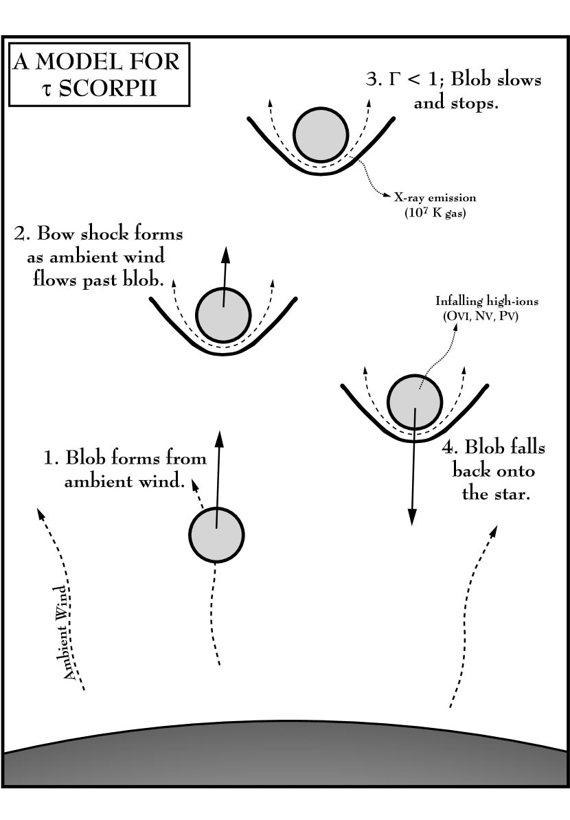
Figure 1: Illustration of the production of X-rays and infalling matter in the form of clumps in the stellar wind of $\tau$ Sco. The clumps are formed from the ambient stellar wind. Because the radiation force is lower than that of gravity ($\Gamma_{e}+\Gamma_{L}<1$), the clumps slow, stop, and then fall back onto the star. The hard X-rays are formed in a bow shock where the wind collides with an infalling clump. The X-rays produce the superionization seen in the UV spectra by way of the Auger ionization mechanism. The wind is also assumed to have the shocks typically asssociated with hot stars; these produce the soft component of the X-ray spectrum of $\tau$ Sco.

A schematic of our model is shown in Figure 1. The basic picture of the stellar wind that we adopt is one in which discrete density enhancements, or clumps, are embedded in an otherwise smooth stellar wind. These dense clumps of material have shock interfaces with the faster moving ambient wind. The most extreme of these clumps are dense enough to be optically thick to radiation in the strongest resonance lines, though still optically thin to UV continuum radiation. In addition to their treatment of stellar winds with organized velocity gradients, the theory of radiative acceleration on material with no internal velocity gradient was developed by Castor, Abbott, & Klein (1975, hereafter CAK), and we use their parameterization of the line-driving force. The equations governing this acceleration are given in §3. Assuming a CAK parameterization of the line driving force, the net radiative acceleration on optically thick parcels of material with no internal velocity gradient can be relatively small (see §3). Gravity dominates the motion of these optically thick clumps, which fall inward, creating bow-shocks at their leading edges as they plow supersonically through the outflowing wind. The velocity structure of the ambient wind is assumed to be relatively unaffected by such clumps. They do not shadow a significant amount of the overlying wind, since they are optically thin to continuum radiation and the line opacity is significantly redshifted relative to the opacity driving the unperturbed wind.

As the clumps fall inward, they shock the out-flowing gas of the ambient (inter-clump) wind. The temperature of gas the immediate post-shock region is proportional to the square of the shock jump velocity as in Equation (1). Since the relevant velocity for the calculation of the shock temperatures in these bow shocks is the relative velocity between the clumps and the ambient wind, the temperatures needed to produce the hard X-ray component observed by ROSAT and ASCA are readily obtained. The X-ray producing shocks adjacent to the leading edge of the infalling clumps produce very highly-ionized material, thus accounting for the red-shifted high ions seen in absorption (O VI, N V, etc.).

A related model was considered by Lucy & White (1980, hereafter LW), in the first paper attempting to explain the source of hot star X-rays as shock-heated gas. They suggested that clumps are radiatively driven outward while the rest of the wind is pushed along by the drag of these objects. In our model the clumps move outward (or inward) with a velocity less than that of the ambient wind, so the shocks occur on the inner face of the clump. This placement of the shocks is more consistent with the results of OCR, who find that shocks tend to be inward facing with low-density, high-speed wind material being driven into slower and denser shocked regions. However, we retain the clump aspect of the LW model.

Let us assume the clumps are self-contained parcels of gas confined by the ram pressure of the wind through which they fall. Following LW, we assume a balance of dynamical pressures and write the average density of a clump, $\langle\rho_{c}\rangle$, falling through the wind as

$$\langle\rho_{c}\rangle=\rho_{w}(r)\frac{(a_{w}^{2}+C_{\rho}\omega^{2})}{a_{c}^{2}}.$$ (2)

In this expression $\rho_{w}$ is the wind density, a function of the distance $r$ from the star, $a_{w}$ and $a_{c}$ are the thermal velocities in the wind and clump, respectively, and $\omega$ is the relative velocity between the wind and the clump. We have ignored the effects of turbulence within the clumps but have included the constant $C_{\rho}=0.29$ as a scale factor to account for the range of angles at which the wind hits the bow-shock (see LW). We can see from this that once a clump begins to decelerate, thereby increasing $\omega$, the oncoming wind confines it more effectively, making it denser as it falls towards the star. This further decreases the ability of the radiation field to drive the clump outwards. If the mass of material accumulated into a clump is specified, then the volume can be readily obtained from the density derived using Equation (2).

This model has the desirable attribute of producing both the red-shifted high-ion absorption and the anomolously hard X-rays. Several independent lines of evidence suggest that clumping can be important in the winds of Wolf-Rayet (e.g., Lépine, Moffat, & Henriksen 1996) and OB supergiant winds (e.g., Sako et al. 1999; Eversberg, Lépine, & Moffat 1998). It is within reason that near main sequence early type stars may also contain localized regions of significantly higher than average densities. The exact mechanism for the formation of these dense clumps is not rigorously approached in this work, but it is worthwhile to explore the consequences of such a model before a more thorough hydrodynamical study is undertaken.

3 INFALLING MATERIAL

The main driving force for winds from massive stars is the radiative acceleration associated with atomic absorption line opacity. The most important of the driving lines are the ultraviolet resonance lines of abundant ionic species. Thus, the driving force is not only dependent upon the elemental abundances in a wind, but also upon the wind’s ionization balance (MacFarlane, Cohen, & Wang 1994; Abbott 1982). The equation of motion describing the trajectory of a parcel of gas with respect to the star is

$${\frac{dv_{c}}{dt}}=-\frac{GM_{*}}{r^{2}}(1-\Gamma_{e}-\Gamma_{L})+f_{d},$$ (3)

where $v_{c}$ is the velocity of the clump of material, $M_{*}$ the mass of the star, $r$ the distance of a clump from its center, and $f_{d}$ is the force per unit mass the ambient wind exerts upon the clump in the form of a “drag.” The terms $\Gamma_{e}$ and $\Gamma_{L}$ are the ratios of the radiative to gravitational acceleration for electron scattering and resonance line scattering, respectively. The drag force, $f_{d}$, is zero if there is no relative motion between a clump and the ambient wind. In this treatment we have not allowed for a thermal pressure gradient in the wind, which is negligible in the supersonic portion of such an outflow.

For the ambient stellar wind, $f_{d}=0$. The requirement for the material to be accelerated away from the star is $dv/dt>0$, implying $\Gamma_{e}+\Gamma_{L}>1$, i.e., that the radiative acceleration is greater than the gravitational acceleration. A dense clump of material formed in the wind that has $\Gamma_{e}+\Gamma_{L}<1$ may decelerate and possibly fall back to the surface of the star, plowing its way through the out-flowing wind as it falls. However, even for clumps with $\Gamma_{e}+\Gamma_{L}<1$, the drag force, $f_{d}$, may be great enough to push the clump outwards in the stellar wind. To determine if infall is physically reasonable, we shall develop more fully each of the terms in Equation (3).

3.1 Radiative Acceleration

The radiative driving force on a parcel of wind material is considered to have two components: radiative driving via electron scattering and resonance line opacities. The radiative acceleration due to electron scattering of the stellar continuum is written

$$g_{e}=\frac{\sigma_{e}F}{c};$$ (4)

here $\sigma_{e}$ is the electron scattering opacity, which is $\sigma_{e}=\sigma_{Th}/\mu_{e}m_{H}\approx 0.34$ cm² g^-1 for $\tau$ Sco, $F$ is the frequency-integrated stellar flux at the location of the material, and $c$ is the speed of light.

A proper treatment of the radiative driving of stellar winds owing to absorption line opacity has been given by CAK (see also Abbott 1982). Their theory paramaterizes the line driving force on a wind having an organized velocity gradient $dv/dr$. In CAK theory, the radiative acceleration due to line scattering, $g_{L}$, is written

$$g_{L}=\frac{\sigma_{e}F}{c}{\cal M}(t)=g_{e}^{\rm ref}{\cal M}(t).$$ (5)

where $g_{e}^{\rm ref}$ is for a reference electron scattering opacity of 0.325 cm² g^-1. So $g_{L}$ is simply the reference electron scattering acceleration modified by a multiplicative factor. This factor, ${\cal M}(t)$, the so-called “force multiplier,” is a function of $t$, an optical depth parameter that is independent of line strength. The force multiplier is defined as

$${\cal M}(t)\equiv kt^{-\alpha}\left(\frac{N_{e}}{W}\right)^{\delta},$$ (6)

where $N_{e}$ is the electron density in units of $10^{11}$ cm^-3, $W$ is the dilution factor and $k,\ \alpha$ and $\delta$ are the CAK parameters. These parameters have been determined from studies employing extensive atomic line lists and depend upon the temperature of the absorbing material (see, e.g., Abbott 1982). However, the driving force for the density enhancements we will consider here is slightly different from the typical CAK driving force for the ambient wind.

In the CAK treatment of expanding atmospheres or winds, $t$ is the electron scattering optical depth over the distance in which the wind velocity increases by the thermal velocity. Hence $t$ is inversely proportional to the local velocity gradient for outflows with monotonically increasing velocity laws (CAK). In the case of parcels of gas with no organized velocity gradient, such as those being considered here, the optical depth parameter $t$ is the integral of the electron scattering opacity over the path length $l$ through the region or clump [Equation (5) of CAK]:

$$t\equiv\sigma_{e}\int_{l}\rho dr.$$ (7)

Approximating the integral as $\langle\rho_{c}\rangle V_{c}^{1/3}$, where $V_{c}\equiv m_{c}/\rho_{c}$ is the volume of the clump, Equation (7) may be rewritten, using Equation (2), as

$$t\approx\sigma_{e}m_{c}^{1/3}\rho_{w}(r)^{2/3}\left(1+\frac{C_{\rho}\omega^{2}}{a_{c}^{2}}\right)^{2/3},$$ (8)

assuming $a_{c}\approx a_{w}$. This latter assumption has the desirable consequence that the density of a clump will approach that of the ambient wind as the relative velocity, $\omega$, approaches zero.

The ratio of the radiative to gravitational accelerations in CAK formalism is written

$$\Gamma_{e}+\Gamma_{L}=\left[\frac{\sigma_{e}L}{4\pi cGM_{*}}\right]\left[1+{\cal M}(t)\right],$$ (9)

given $L$, the luminosity of the star. We will assume the values of the CAK parameters tabulated by Abbott (1982) for stellar winds at 30,000 K ($k=0.156,\ \alpha=0.609$ and $\delta=0.12$) are appropriate for use in the clumps considered here. These are the same as those used for estimating the mass loss rate. Given the high densities predicted for the clumps and the presence of a hard X-ray source at their leading edges, the ionization balance in the clumps could be different than that of the ambient wind. Thus while the CAK parameters appropriate for the clump may be different than those used here, we adopt these parameters in order to proceed. In the end, the choice of CAK parameters will likely not matter too much so long as the optical depth through a clump is very high. Equation (9) gives an upper limit to the radiative acceleration because it assumes that the flux from the star reaching a parcel of gas is unattenuated by the layers closer to the star. For a clump moving outwards at lower velocities than the ambient wind, the photons producing the line radiation pressure on the dense clump may already have been absorbed or scattered by gas lower in the wind with the same outward velocity as the clump. We will ignore this effect here, which is expected to be small.

3.2 Drag force

The standard drag force per unit mass on a clump of area $A_{c}$ moving through an ambient medium with a relative velocity $\omega$ is given by

$$f_{d}=\frac{1}{2}C_{D}\rho_{w}(r)\omega^{2}\left(\frac{A_{c}}{m_{c}}\right).$$ (10)

In this treatment $m_{c}$ is the mass of the clump, and $\rho_{w}(r)$ is the density of the ambient medium (in this case the ambient stellar wind). The drag coefficient, $C_{D}$, dictates the efficiency of momentum transfer to the clump, and the factor of $\text@frac{1}{2}$ is conventionally included. This expression describes the energy density impinging on the clump integrated over the area of the clump. For most of this work we will assume $C_{D}=2$, i.e., perfect transfer of momentum from the ambient wind to the clump. This is the most stringent assumption for determining if infall is viable.

The cross section of the clump may be approximated $A_{c}\approx V_{c}^{2/3}$, giving

$$f_{d}=\frac{\frac{1}{2}C_{D}\rho_{w}\omega^{2}}{\left(m_{c}\langle\rho_{c}\rangle^{2}\right)^{1/3}}.$$ (11)

Using Equation (2), and assuming $a_{c}\approx a_{w}$ and $\omega\gg a_{c}$, we rewrite this as

$$f_{d}\approx\frac{1}{2}C_{D}\left(\frac{a_{c}^{4}\,\rho_{w}\omega^{2}}{C_{\rho}^{2}\,m_{c}}\right)^{1/3}.$$ (12)

The density of the wind at a distance $r$ from the surface of the star is calculated assuming mass conservation:

$$\rho_{w}(r)=\frac{\mbox{\.{M}}}{4\pi r^{2}v_{w}(r)},$$ (13)

where Ṁ is the mass loss rate (see Table 1). The velocity of the wind $v_{w}(r)$ is calculated using a $\beta$ velocity law with $\beta_{w}=0.8$ (Groenewegen & Lamers 1989):

$$v_{w}(r)=v_{\infty}\left(1-\frac{R_{*}}{r}\right)^{\beta_{w}}.$$ (14)

with the values of $v_{\infty}$ and $R_{*}$ given in Table 1.

The magnitude of the drag force can be relatively small. We estimate its magnitude using Equations (12) and (13) with the data given in Table 1:

$$f_{d}\approx 55\ \mathrm{cm\ s^{-2}}\ \left(\frac{r}{R_{*}}\right)^{-2/3}\left(\frac{m_{c}}{10^{19}\,{\mathrm{g}}}\right)^{-1/3}v_{w}(r)^{1/3},$$ (15)

where we have assumed $\omega=v_{w}$, which in this equation is in units km s^-1. If we define $\Delta\equiv f_{d}/g$, where $g$ is the force of gravity per unit mass, we can rewrite Equation (3) as $dv_{c}/dt=-g(1-\Gamma_{e}-\Gamma_{L}-\Delta)$. We find

$$\Delta\approx 6\times 10^{-3}\ \left(\frac{r}{R_{*}}\right)^{4/3}\left(\frac{m_{c}}{10^{19}\,{\mathrm{g}}}\right)^{-1/3}v_{w}(r)^{1/3},$$ (16)

where $v_{w}$ is again in km s^-1. We can see that very near the star, the drag force is relatively small compared with the force of gravity because the velocity between the clump and the ambient wind is smaller than at larger radii. This prediction is based on the assumption $\omega\approx v_{w}$, but for clumps producing temperatures in excess of $10^{7}$ K, our numerical calculations discussed in §3.3 suggest the drag force is much more significant (relative to gravity) at larger radii. For clumps with masses $\log m_{c}\approx 20.0$ (in grams) the outward drag force is comparable to the force of gravity at large distances ($r>10R_{*}$) from the stellar surface. For lower mass clumps, however, the drag force can play an important role in the dynamics at intermediate distances from the star ($r\sim 5R_{*}$).

3.3 Numerical Results

We have derived the individual components of Equation (3), and can hence obtain trajectories in position-velocity space for clumps in the wind of $\tau$ Sco. Equation (3) shows the dynamics of such clumps depend on the relative velocity, $\omega$, between the clump and the ambient wind: $\omega\equiv v_{w}(r)-v_{c}$, where $v_{w}(r)$ and $v_{c}$ are the wind and clump velocities, respectively. We have numerically integrated the equation of motion for parcels of gas with various initial conditions since it does not have a analytically tractable solution. The initial conditions specified in our approach are the initial distance $r_{\circ}$ from the center of the star, the initial relative velocity $\omega_{\circ}$, and the mass $m_{c}$ of the clump (we assume mass conservation). By specifiying $\omega_{\circ}$ and $r_{\circ}$, we are also then specifying the initial velocity of the clump, given Equation (14). We assume the value of $\omega_{\circ}$ is characteristic of the jump velocities typically seen in numerical simulations, i.e., $\Delta v\lesssim v_{w}/2$ (Cooper 1994). The dependence on $m_{c}$ comes in through Equations (8) and (12), the former affecting ${\cal M}(t)$ in the radiative acceleration.

Our numerical integrations of the equation of motion show two types of clump trajectories: outflow and infall trajectories. We term those trajectories in which the clumps are driven from the star, though they may initially decelerate, outflow trajectories. Though these clumps are driven outward, they always have velocities less than the terminal velocity of the wind. Those that decelerate and eventually descend towards the star follow infall trajectories. The latter type is the most interesting, given the redshifted high ion absorption line observations. It is not clear, however, that outflow and infall trajectories are mutually exclusive. There may exist a mix of trajectories based upon a distribution of initial conditions for the clumps. Figure 2 displays the velocity of representative outflow and infall trajectories as a function of distance from the star. Also shown is the adopted $\beta$ velocity law of the wind.

To demonstrate the sensitivity of these trajectories to initial conditions, we have compiled a series of trajectories that are different in only one of the three possible input conditions. Figure 2 shows the trajectories of clumps with $r_{\circ}=1.20\ R_{*}$ and $\omega_{\circ}=v_{w}/2=331$ km s^-1; the masses of the clumps in this figure are $\log m_{c}=18.0,$ 19.0, 19.5, and 20.0 ($m_{c}$ in grams). The low-mass clumps are driven outward through the wind while the high-mass objects relatively quickly stop and start to descend towards the star. The low-mass clumps continue outwards because of their lower column density (and correspondingly low $\tau_{L}$), allowing for more effective radiation driving. Lower-mass clumps are also more effectively pushed outwards by the drag force provided by the on-rushing stellar wind, though this is usually minor compared with the force provided by resonance line scattering of radiation. Figure 3 shows trajectories for clumps having the same mass and initial velocity relative to the wind [$(\log m_{c},\ \omega_{o})=(19.0,\ 250\ \mathrm{km\ s^{-1}})$] but with starting positions $r_{o}=1.10$, 1.15, 1.20, and 1.25 $R_{*}$; and in Figure 4 we show trajectories for clumps having a mass $\log m_{c}=19.0$ starting at $r_{o}=1.20\ R_{*}$ with initial velocities relative to the wind of $\omega_{o}=100$, 200, 300 and 400 km s^-1. Clumps with larger $\omega_{o}$ tend to fall in more readily than those with low $\omega_{o}$, as parcels of gas with smaller initial distances from the stellar surface, $r_{o}$, are also more likely to fall inwards. We note that the factor $C_{\rho}=0.29$ included in Equation (2) is not well known. If this constant were larger, the clumps in our models would be more effectively confined and have higher densities. This would make it easier for a clump of given initial conditions to fall inwards.

In Table 2 we give several properties for trajectories with a range of initial conditions. Included in the table are the initial conditions $\omega_{o}$, $r_{o}$, and $\log m_{c}$. Also given is the lifetime ${\cal T}$ of the clump, in hours, the final velocity of the clump in our calculations, the maximum relative velocity between the clump and the stellar wind, $\omega_{max}$, and the corresponding maximum shock temperature. For the outflow trajectories, the final velocity is the velocity of the clump at a distance of $10R_{*}$ from the surface of the star, and the lifetime is the time it takes to reach this point.

It is clear from Figures 2–4 that conditions for infall can be met for a broad range of initial conditions. Our hypothesis that the infall of material may be responsible for the observed red-shifted component of the high-ionization lines is thus reasonable. Table 2 shows that many combinations of initial conditions can yield infall trajectories. Infall velocities of $\sim 300$ km s^-1 (as observed in the red wings of the O VI lines) are found for clumps with masses in excess of $\sim 10^{19}$ grams. Clumps originating at larger distances from the star reach higher infall velocities. Clumps following infall trajectories spend more time near their “turning point,” i.e., where $v_{c}\simeq 0$, than close to the photosphere where their infall velocity reaches its maximum. The observed O VI profiles require this, showing absorption consistent with a Gaussian optical depth distribution centered at $v_{c}\simeq 0$ km s^-1 relative to the photosphere.

Typical lifetimes for clumps following infall trajectories are $\simeq 3-10$ hours, while outflow trajectories take $15-30$ hours to reach $r\approx 10R_{*}$. In general clumps with initial distances $r_{\circ}\gtrsim 1.2R_{*}$ with $\omega_{\circ}=0.5v_{w}(r_{\circ})$ require masses of order $\log m_{c}\gtrsim 19.1$ to achieve infall. The highest-temperature gas is produced for clumps that reach the largest distances from the stellar surface. Thus lower mass clumps starting at relatively large distances from the star produce the hardest X-rays. One can see from Table 2 that the trajectories followed by high-density clumps with $\log m_{c}=19.5$ tend to produce slightly harder X-rays than those with $\log m_{c}=18.0$ or 20.0. We believe the most likely clump masses for $\tau$ Sco are in the range $\log m_{c}=19.0$ to 19.5 (in grams) given their ability to infall and produce very hot gas.

For infall trajectories $\omega_{max}$ occurs near the turn-around point in a cloud’s trajectory. Specifically, the largest velocity jumps are usually found immediately after a clump of material has begun to fall inwards. At this point the parcel of gas is at the maximum height above the star, and the ambient wind velocity is larger than at any other point in the clump’s trajectory. Though clumps may accelerate as they near the star, the decrease in the wind velocity with distance from the stellar surface offsets this increase in the infall velocity of the material.

4 X-RAY EMISSION

4.1 Temperature Distribution

Having shown that the interpretation of the red-shifted high-ion absorption as infall is a physically reasonable one, we now approach the anomolous X-ray spectrum for $\tau$ Sco. We have speculated that the observed X-rays are a by-product of the interaction of infalling clumps with the outgoing wind. The temperature $T_{s}$ for gas in a section of a bow shock can be calculated by substituting $v_{s}\cos\theta$ for $\Delta v$ in Equation (1), where $v_{s}$ is the shock-jump velocity (here the relative velocity between the wind and a clump, $\omega$) and $\theta$ is the angle at which the material enters the shock, relative to a ray normal to the shock’s surface. The temperature of gas is a function of position along the shock’s leading edge, via the $\theta$ dependence. Calculating the true run of temperatures requires knowledge of the exact shape of the bow-shock. This is an inherently difficult problem and is beyond the scope of this work. When discussing the temperatures produced by our infalling parcels of gas, we will typically give results that assume $\theta=0^{\circ}$, and, following LW, values corresponding to the shock at $\theta=30^{\circ}$. Truth may be somewhere between these values for the majority of the shocked gas.

The trajectories calculated in §3.3 permit us to estimate the bow-shock temperature at each point of a clump’s history given its velocity relative to the ambient wind. It is clear that the infall velocities of the trajectories displayed in Figures 2–4 can exceed $\sim 300$ km s^-1, sometimes approaching $\sim 500$ km s^-1 near the base of the wind. As mentioned in §3.3, the relative velocity between the wind and the infalling clumps can be much higher than these values. The maximum relative velocities in the trajectories for clouds having $\log m_{c}=18.0$, 18.5, 19.0, and 19.5 in Figure 2 are $\omega_{max}\approx 1460,$ 1660, 1295, and 1202 km s^-1. These velocities imply maximum shock temperatures of order $T_{s}\approx(31,\ 40,\ 24,\ \mathrm{and}\ 21)\times 10^{6}$ K, respectively, well in excess of the temperatures required to match the CCW and Cassinelli et al. (1994) fits. Even the outflow trajectories provide very large velocity jumps, and hence large shock-jump temperatures. If we assume $\Delta v=\omega\cos 30^{\circ}$ we find $T_{s}\approx(5-10)\times 10^{6}$ K. This is still quite close to the temperatures required to explain the ASCA observations of CCW.

Figures 5 and 6 show two trajectories as well as the model temperature distribution of the shock-heated gas. The initial conditions for the trajectory shown in Figure 5 are $(\log m_{c},\ r_{o},\ \omega_{o})=(19.0,\ 1.3\ R_{*},\ 371\ \mathrm{km\ s^{-1}})$, while those for Figure 6 are $(\log m_{c},\ r_{o},\ \omega_{o})=(19.0,\ 1.5\ R_{*},\ 498\ \mathrm{km\ s^{-1}})$; in each case $\omega_{\circ}=v_{w}/2$. Changing the initial height above the stellar surface between these two figures causes the clump to flow outwards in the wind. The maximum shock temperatures expected from these two trajectories are near $5\times 10^{6}$ K. The insets show the expected relative temperature distribution over the lifetime of the clump. These distributions have been weighted by $\rho_{w}(r)^{2}$ for each point in the clumps’ trajectories to approximately account for the expected differences in the X-ray emission measure at different points in the wind. We show both the distribution assuming $\theta=0^{\circ}$ (solid histogram) and $\theta=30^{\circ}$ (dotted histogram) in these figures.

The temperature distributions shown in Figures 5 and 6 show that the trajectories of dense parcels of gas derived in §3 provide large enough shock-jump velocities to produce gas in excess of $10^{7}$ K. This treatment is very approximate. For instance we have neglected the cooling of the gas in the bow shocks around the clumps. The gas that is heated to $T\sim 10^{7}$ will eventually cool through the lower X-ray emitting temperatures, providing for enhanced emission in the soft X-ray bands over that shown in Figures 5 and 6. Though the temperature distributions peak at the same temperatures, the temperature distribution for the infall trajectory (Figure 5) is narrower than that of the outflow trajectory (Figure 6), which shows a strong tail towards higher temperatures. The ratio of the emission measures of X-ray emitting gas observed by CCW at (1.2 and $2.4)\times 10^{7}$ K is $\lesssim 3.5$. Both the outflow and infall trajectories have similar displayed in these figures produce X-ray emitting material at (1.2 and $2.4)\times 10^{7}$ K in a ratio of 1.9:1. This value is consistent with the observational constraints, though the effects of radiative and adiabatic cooling will affect the final distribution of X-ray emission.

In all likelihood a population of clumps in the wind of $\tau$ Sco will have a range of initial conditions, providing a range of X-ray producing temperatures and X-ray luminosities per clump. The distribution of intial conditions, the true shape of the bow shock at the leading edges of the infalling clumps, and the cooling of the post-shock gas will all determine the true temperature and luminosity distribution of X-ray emitting gas. The derivation of these factors is beyond the scope of this paper. Our goal is to show that the production of very hot gas, in excess of $10^{7}$ K, is possible in the wind of $\tau$ Sco through the infall of dense material. Our dynamical modelling of the dense clumps in §3 has shown that infall can occur. The discussion presented in this section shows that the infall can create the requisite conditions for producing this very hot gas

4.2 X-ray Luminosity and the Number of Clumps

The X-ray luminosity predicted in our model is also reasonable. The mechanical luminosity of the wind $L_{w}\sim\text@frac{1}{2}\mbox{\.{M}}v_{\infty}^{2}$ is a factor of $\sim 780$ greater than $L_{X}$ for this star. Even if we assume the appropriate velocity for use is not the full terminal velocity, but rather $\sim 1500-2000$ km s^-1, similar to the observed wind velocities at distances typical of our model clumps, we still have $L_{w}\sim 300-600L_{X}$. Thus the ensemble of clumps need only convert $<1\%$ of the wind mechanical luminosity to X-ray luminosity to match the observed $L_{X}$.

We estimate the available luminosity, $L_{c}$, for X-ray production from a single clump as $L_{c}\simeq\text@frac{1}{2}\rho_{w}\omega^{3}A_{c}$. The trajectory in Table 2 with initial conditions $(\log m_{c},\ r_{o},\ \omega_{o})=(19.0,1.20\ R_{*},\ 286\ \mathrm{km\ s^{-1}})$ reaches a maximum height of $\sim 1.5\ R_{*}$ with a relative velocity $\omega\sim 1000$ km s^-1 at this height. This clump will have an area $A_{c}\simeq 3\times 10^{20}$ cm² at its maximum height, and we find $L_{c}\simeq 5\times 10^{29}$ ergs s^-1. Thus of order $\sim 150$ individual clumps, assuming perfect efficiency, are required to produce the observed X-ray luminosity of the star, $L_{X}\approx 7.3\times 10^{31}$ ergs s^-1 (Cohen, Cassinelli, & MacFarlane 1997; hereafter CCM). If we assume an efficiency of $\sim 10-20\%$ for conversion of kinetic energy to X-ray luminosity in the ROSAT bandpass (see, e.g., Wilson & Raymond 1999), then the total number of clumps required by the X-ray observations is of order $10^{3}$. The observed luminosity of the hard component is significantly lower than the total ($L_{X}\sim 1.8\times 10^{31}$ ergs s^-1; CCW), in qualitative agreement with the temperature distributions shown in the insets of Figures 5 and 6.

We can estimate a lower limit to the number of clumps from the lack of (short-term) variability in the observed X-rays (CCM). The population of clumps that exist in the wind at any one time ($N$) should be large enough to produce X-ray variations less than $\sqrt{N}/N\lesssim 0.04$, or $N\gtrsim 600$ clumps. Assuming 600 clumps of mass $\log m_{c}\approx 19.0$ with lifetimes similar to those in Table 2, ${\cal T}\sim 5-11$ hours, this yields a creation rate of mass in clumps of $\mbox{\.{M}}^{create}_{c}\sim(2-5)\times 10^{-9}$ M_⊙ yr^-1. Assuming half of the clumps actually escape in the wind (follow outflow trajectories), the mass loss rate in clumps is $\mbox{\.{M}}_{c}\sim(1-3)\times 10^{-9}\ \mbox{{M${}_{\odot}$ yr${}^{-1}$}},or\sim 10\%$ of Ṁ.

Another constraint on the number of clumps residing in the stellar wind of $\tau$ Sco comes from the O VI absorption line profile. The $\lambda 1038$ Å profile shows $\sim 10\%$ absorption near $v\sim 0$ km s^-1. Assuming the O VI optical depth for an individual clump is much larger than unity and, as above, that the clumps are at a distance $r\sim 1.5\ R_{*}$ with mass $\log m_{c}\approx 19.0$, approximately $N_{c}\sim 1900$ clumps are required to cover 10% of the total solid angle of the star. This corresponds to a mass loss rate of $\mbox{\.{M}}=(0.8-2.0)\times 10^{-8}$ M_⊙ yr^-1 for assumed lifetimes ${\cal T}\sim 5-11$ hours. If the efficiency of mechanical to X-ray luminosity from the previous paragraph is $\sim 10\%$, these two estimates of the number of clumps are in agreement. It is worth noting that the infall trajectories are naturally weighted to provide more absorption near $v_{c}\sim 0$ km s^-1, i.e., near the upper-most point in the trajectory, than at larger infall velocities. This can be seen in Figure 5 where we have plotted a dot every 1.25 hours along the clump’s trajectory. The high density of dots near the turning points implies that a random sample of clumps drawn from from this trajectory will be heavily weighted towards low velocities, in agreement with the Gaussian shape of the O VI absorption. Detailed line-profile calculations will be the subject of a future work.

Our calculations suggest that the required number of clumps in the wind of $\tau$ Sco is of order $10^{3}$, with Ṁ_c approximately $\mbox{a few }\times 10^{-9}$ M_⊙ yr^-1, consistent with the adopted mass loss rate of this star. These rough numbers can vary significantly depending on the assumptions made, however. At the present time there is no clear evidence for an inconsistency with the observational constraints. Further work will need to place more stringent constraints on the allowable parameters of this model.

5 WHY $\tau$ SCO?

Though our simple model can explain several of the observational aspects of the stellar wind of $\tau$ Sco, there are several questions and details that we have not approached. Principal among these is what makes $\tau$ Sco so special? Why do most hot stars not show the observed peculiarities of this star? This is may be due to the special location of $\tau$ Sco on the main sequence where the mass loss rate steeply drops with $T_{\rm eff}$. Main sequence stars hotter than B0, i.e., the main sequence O stars, have mass loss rates considerably higher than $\tau$ Sco. For instance, the mass loss rate of O9 V stars with $T_{\rm eff}\simeq 35,000$ K, $L\simeq 10^{5}L_{\odot}$, and $M\simeq 25M_{\odot}$ are of order $10^{-7}$ M_⊙ yr^-1 (predicted by the CAK theory), compared with less than $10^{-9}$ or $10^{-10}$ M_⊙ yr^-1 for B1.5 and later stars. This is observed in the sudden disappearance of the P Cygni profiles of the UV resonance lines in stars between O9.5V and B0.5V (see the atlas of UV line profiles of Snow et al. 1994). The mass loss rates of B1.5 V stars are typically a factor of $\sim 10$ below $\tau$ Sco (e.g., the stars in CCM), with B2 star mass loss rates often being a factor of 100 lower than that adopted for $\tau$ Sco.

We speculate that the prevailing conditions for stars near the position of $\tau$ Sco in the HR diagram are just right not only for the formation of dense clumps of material within the wind, but also for their ability to infall. Stellar winds near the spectral type of $\tau$ Sco are only marginally able to be driven by the radiation of the underlying stars. Clumps with no organized velocity gradient formed in such winds are less likely to be pushed outward than in the winds of earlier-type stars.

To investigate the differences between $\tau$ Sco and earlier-type O stars, we have calculated trajectories for high-density clumps in the wind of the O9 V star 10 Lacertae. We adopt stellar parameters given in Brandt et al. (1998) and Snow et al. (1994) in our calculations: $L_{*}=10^{5}\ L_{\odot}$, $M_{*}=25$ M_⊙, $R_{*}=8.3\ R_{\odot}$, $\mbox{\.{M}}=1.6\times 10^{-7}$ M_⊙ yr^-1, $T_{eff}=36,000$ K, and $v_{\infty}\equiv 2.6v_{esc}=2520$ km s^-1. We note that like $\tau$ Sco, 10 Lac has a low projected rotation velocity ($v\sin i\approx 40$ km s^-1). We find no infall trajectories for initial distances from the stellar surface $r_{o}\gtrsim 1.03\ R_{*}$, initial relative velocities $\omega_{o}\lesssim 0.5v_{w}(r_{o})$, and masses in the range $\log m_{c}<21.0$. This is primarily a function of the increased luminosity to mass ratio of the star, though the extra drag force plays a limited role. This explains the lack of red-shifted absorption components of O VI in the spectrum of 10 Lac.

Our calculations show that clumps in the wind of 10 Lac will have shock jump velocities in excess of 1000 km s^-1, producing temperatures in excess of $10^{7}$ K. This is very close to the value of $0.5v_{w}$ found for shocks in “normal” stellar winds. The emission from (outflowing) clumps in the wind of 10 Lac will be indistinguishable from the normal X-ray flux due to shocks in unstable stellar winds of O-stars.

The lack of redshifted absorption profiles in the UV lines of main sequence stars of spectral type B0.5 and later is due to drastic decrease in mass loss. A simple scaling of the optical depth of the O VI lines by a factor 0.1 compared to $\tau$ Sco, due to a ten times lower mass loss rate, makes these lines undetectable in the Copernicus spectra, though few such stars were observed with Copernicus. The significantly lower mass loss rates of later-type stars may not provide the requisite conditions for formation of an ensemble of clumps like those thought to exist in the wind of $\tau$ Sco. In general we would expect fewer, lower mass, clumps to form in the winds of later type stars. Such clumps would be less dense than their counterparts in the wind of $\tau$ Sco, hence more likely to flow outward. In the winds of later-type B stars, with significantly lower densities and terminal velocities, the clumps would produce lower temperature and lower luminosity X-rays, perhaps undetectable or indistinguishable from the expected shock emission.

6 SUMMARY

We have outlined a model to explain the two peculiar observational properties of the stellar wind of $\tau$ Sco: infall of high-density clumps surrounded by very highly-ionized gas that gives rise to the red-shifted absorption wings of the O VI lines, and strong shocks that produce the hard X-ray spectrum.

Our model hypothesizes that density enhancements in the stellar wind lead to the formation of dense clumps of material, confined by ram pressure, that decouple from the dynamical flow of the ambient stellar wind. These clumps have very large optical depths in the UV resonance lines responsible for driving the stellar wind. The resulting radiative acceleration of the clumps is insufficient to overcome the gravity, so they slow down and fall back towards the star. As they do so, their interaction with the on-rushing stellar wind produces a bow shock, with shock temperatures reaching several times $10^{7}$ K.

We have presented detailed dynamical models of density enhancements in the wind of $\tau$ Sco, which show that infall can be achieved for a wide range of initial conditions. Using these trajectories we have shown that the shock-jump velocities can approach 2000 km s^-1. The anomolously hard X-rays observed from $\tau$ Sco by Cassinelli et al. (1994) and CCW are produced in these bow shocks at temperatures of $\sim(1-5)\times 10^{7}$ K. The infalling high-ionization material observed in the O VI doublet by Lamers & Rogerson (1978) is material in and around the infalling clumps that is ionized by the hard X-rays produced in the bow shocks at the clumps’ leading edges.

Our calculations show that clumps with masses in the range of $10^{19}$ to $10^{20}$ g will fall back if they are formed at radii $\lesssim 1.3\ R_{*}$ (see Table 2). Only the clumps formed above 1.1 $R_{*}$ produce shocks with temperatures in excess of $10^{7}$ K. Clumps formed this high have maximum infall velocities of order 500 km s^-1. This is higher than the observed maximum redshift of 250 km s^-1, but the clumps spend very little time at such high velocities. Even clumps with a large final infall velocity will give the maximum contribution to the the UV line profile at small velocities, because they spend much more time near their turning point, where $v\simeq 0$, than at high velocity just before they disappear into the photosphere. This explains why the O VI absorption reaches a maximum near 0 km s^-1.

We estimate that $\gtrsim 10^{3}$ clumps of mass $10^{19}-10^{20}$ g are needed to explain the observed O VI absorption lines and the hard X-ray flux. This corresponds to a clump mass loss rate of Ṁ${}_{clumps}\sim 1-5\times 10^{-9}\ \mbox{{M${}_{\odot}$ yr${}^{-1}$}},or\sim 0.1\ \mbox{\.{M}}_{wind}$. In making these estimates we have assumed several efficiency factors whose values are not well known at present and would require detailed modelling to be improved. For instance, (a) in comparing the predicted X-ray luminosities with observations we have assumed a perfect conversion of ram pressure heating to X-ray emission; (b) we have neglected the radiative cooling of shocks which may result in a reduction of the predicted X-ray flux from an individual clump; and (c) we have assumed that the clumps are optically thick in the O VI transitions, and that the intrinsic line widths of the clumps is sufficient to account for the breadth of the observed absorption. A reduction in these “efficiencies” may result in an increase in the required number of clumps. This will be the subject of a subsequent study.

We explain the special situation of $\tau$ Sco in terms of its location on the main sequence where the mass loss rate drops by about factor 100 from O9 V to B1 V. This can be tested and our model can be improved by high S/N observations of the far UV resonance lines of O VI, S VI, and P V of a number of O9.5 V to B1 V stars with the Far Ultraviolet Spectroscopic Explorer (FUSE). This satellite will cover the wavelength range $905-1197$ Å and will observe a large number of early-type stars. Our model would suggest that stars with spectral types similar to $\tau$ Sco should also show infall in the O VI doublet at $\lambda\lambda 1032$ and 1038 Å, which will be well observed with FUSE.

The dynamical model developed in this work can be generally applied to clumps in line-driven outflows. Though it seems that the properties of stars near $\tau$ Sco on the HR diagram may be the best for producing infalling clumps with recognizable observational consequences, clumping may occur in many types of early-type stellar winds, and may also be important in outflows from extragalactic sources (e.g., AGNs and QSOs). The dynamical model described here can be applied to all of these cases (as discussed for the case of 10 Lac above).

Table 1: Stellar Parameters for $\tau$ Scorpii

Quantity	Value	Source
Spectral Type	B0.2 V	Walborn(1994)
Distance (pc)	132	Hipparcos (Perryman et al. 1998)
$V$ (mag)	2.82	Hipparcos (Perryman et al. 1998)
$N_{\rm HI,\,ISM}$ (cm-2)	$2.9\times 10^{20}$	Diplas & Savage (1994)
$T_{\rm eff}$ (K)	31,400	Kilian (1992)
$R_{*}$ ($R_{\odot}$)	6.5	Snow et al. (1994)
$M_{*}$ ($M_{\odot}$)	15	Snow et al. (1994)
$v_{esc}$ (km s-1)	917	Snow et al. (1994)
$L_{*}$ (ergs s-1)	$1.4\times 10^{38}$	Snow et al. (1994)
$L_{X}$    (ergs s-1)	$7.3\times 10^{31}$	Cohen et al. (1997)
$v\sin i$ (km s-1)	20	Uesugi and Fukuda (1982)
Ṁ    (M⊙ yr-1)	$3.1\times 10^{-8}$	This work
$v_{\infty}$    (km s-1)	2400	This work

Table 2: Properties of Clump Trajectories

$\log m_{c}$	$r_{o}$	$\omega_{o}$	$v_{w}(r_{o})$	${\cal T}$	$v_{b,\,final}$	$\omega_{max}$	$T_{s,\,max}$
[g]	[$R_{*}$]	[km s-1]	[km s-1]	[hrs.]	[km s-1]	[km s-1]	[$10^{6}$ K]
18.0	1.10	176	352	06.3	$-230$	0730	08
18.0	1.25	331	662	22.4	$+790$	1460	31
19.0	1.10	176	352	02.8	$-270$	0580	05
19.0	1.15	235	470	04.5	$-340$	0820	10
19.0	1.20	286	572	06.8	$-400$	1055	16
19.0	1.25	331	662	11.2	$-450$	1295	24
19.0	1.30	371	742	25.9	$-490$	1590	36
19.0	1.50	498	996	25.1	$+540$	1670	40
19.5	1.10	176	352	02.5	$-280$	0560	05
19.5	1.15	235	470	03.8	$-355$	0785	09
19.5	1.20	286	572	05.5	$-415$	1000	14
19.5	1.25	331	662	07.9	$-470$	1202	21
19.5	1.30	371	742	11.8	$-515$	1405	28
19.5	1.50	498	996	33.7	$+385$	1820	48
20.0	1.10	176	352	02.3	$-285$	0555	04
20.0	1.20	286	572	04.8	$-430$	0970	13
20.0	1.30	371	742	09.3	$-530$	1340	26
20.0	1.50	498	996	58.5	$+300$	1990	57

Figure 2: Trajectories of clumps forming in the wind of $\tau$ Sco having different initial conditions. The velocity scale is relative to the surface of the star, and the distance from the stellar surface is given in units of stellar radii. Also shown is the $\beta$ velocity law of the ambient stellar wind (solid line). The starting distance from the star and velocity relative to the ambient wind for these clumps are $(r_{o},\ \omega_{o})=(1.25\ R_{*},\ 331\ \mathrm{km\ s^{-1}})$. The four different trajectories represent clumps formed with masses $\log m_{c}=18.0$, 18.5, 19.0, and 19.5 ($m_{c}$ in grams). The masses are labelled for each trajectory. Note the low-mass clumps are pushed outwards through the wind, following outflow trajectories. The higher mass clumps are able to fall back onto the star and follow infall trajectories.

Figure 3: As Figure 2, but for clumps of constant mass and initial velocity relative to the wind [$(\log m_{c},\ \omega_{o})=(19.0,\ 250\ \mathrm{km\ s^{-1}})$] with varying initial radii [$r_{o}=1.10,\ 1.20,\ 1.25,\ \mathrm{and}\ 1.30\ R_{*}$]. The initial radii are labelled for each trajectory.

Figure 4: As Figure 2, but for clumps of constant mass and initial radii [$(\log m_{c},\ r_{o})=(19.0,\ 1.25\,R_{*})$] with varying initial relative velocities [$\omega_{o}=150,\ 250,\ 300,\ \mathrm{and}\ 400\ \mathrm{km\ s^{-1}})$]. At this position in the wind, $\text@frac{1}{2}v_{w}=331$ km s^-1. The initial relative velocities are labelled for each trajectory.

Figure 5: The main plot shows a trajectory for a clump with the initial conditions $(\log m_{c},\ r_{o},\ \omega_{o})=(19.0,\ 1.30\ R_{*},\ 371\ \mathrm{km\ s^{-1}})$. This clump follows an infall trajectory. The trajectory is marked with a dot every 1.25 hours. Also shown is the wind velocity calculated with a $\beta$ velocity law (dot-dashed line). The inset shows the relative distribution of temperatures in the shock-heated gas formed as the clump follows this trajectory. This distribution is weighted by $\rho_{w}(r)^{2}$ for each point along the trajectory to roughly account for the dependence of the X-ray emission on density. The shock-jump velocities, $\Delta v$, are calculated from the relative velocity between wind and the clump, $\omega$, such that $\Delta v=\omega\cos\theta$. The solid distribution of temperatures assumes $\theta=0^{\circ}$, while the dotted distribution uses $\theta=30^{\circ}$.

Figure 6: As for Figure 5, but for the initial conditions $(\log m_{c},\ r_{o},\ \omega_{o})=(19.0,\ 1.50\ R_{*},\ 498\ \mathrm{km\ s^{-1}})$. This clump follows an outflow trajectory.

References

- (1)
- (2) Abbot, D.C. 1982, ApJ, 259, 282
- (3)
- (4) Bjorkman, J.E., & Cassinelli, J.P. 1993, ApJ, 409, 429
- (5)
- (6) Brandt, J.C. et al. 1998, AJ, 116, 941
- (7)
- (8) Cassinelli, J.P., Cohen, D.H., MacFarlane, J.J., Sanders, W.T., & Welsh, B.Y. 1994, ApJ, 421, 705
- (9)
- (10) Cassinelli, J.P., & Swank, J.H. 1983, ApJ, 271, 681
- (11)
- (12) Castor, J.I., Abbot, D.C., & Klein, R.I. 1975, ApJ, 195, 157
- (13)
- (14) Chlebowski, T., Harnden, F.R., & Sciortino, S. 1989, ApJ, 341, 427
- (15)
- (16) Cohen, D.H., Cassinelli, J.P., & MacFarlane, J.J. 1997, ApJ, 487, 867 (CCM)
- (17)
- (18) Cohen, D.H., Cassinelli, J.P., & Waldron, W.L. 1997, ApJ, 488, 397 (CCW)
- (19)
- (20) Cooper, R.G. 1994, Ph.D. Thesis, Univ. Delaware
- (21)
- (22) Diplas, A., & Savage, B.D. 1994, ApJS, 93, 211
- (23)
- (24) Eversberg, T., Lépine, S., & Moffat, A.F.J. 1998, ApJ, 494, 799
- (25)
- (26) Feldmeier, A. 1995, A&A, 299, 523
- (27)
- (28) Gathier, R., Lamers, H.J.G.L.M., & Snow, T.P. 1981, ApJ, 247, 173
- (29)
- (30) Groenewegen, M.A.T., & Lamers, H.J.G.L.M. 1989, A&A, 79, 359
- (31)
- (32) Hamann, W.R., 1981, A&A, 100, 169
- (33)
- (34) Kilian, J. 1992, A&A, 262, 171
- (35)
- (36) Kudritkzi, R.P., Pauldrach, A., Puls, J., & Abbot, D.C. 1989, A&A, 219, 205
- (37)
- (38) Lamers, H.J.G.L.M., & Pauldrach, A. 1991, A&A, 244, L5
- (39)
- (40) Lamers, H.J.G.L.M., & Rogerson, J.B. 1978, A&A, 66, 417
- (41)
- (42) Lépine, S., Moffat, A.F.J., & Henriksen, R.N. 1996, ApJ, 466, 392
- (43)
- (44) Lucy, L.B. 1982, ApJ, 255, 286
- (45)
- (46) Lucy, L.B., & White, R.L. 1980, ApJ, 241, 300 (LW)
- (47)
- (48) Lucy, L.B., & Solomon, P.M. 1970, ApJ, 159, 879
- (49)
- (50) MacFarlane, J.J., & Cassinelli, J.P. 1989, ApJ, 347, 1090
- (51)
- (52) MacFarlane, J.J., Cohen, D.H., & Wang, P. 1994, ApJ, 437, 351
- (53)
- (54) Massa, D., Savage, B.D., & Cassinelli, J.P. 1984, ApJ,
- (55)
- (56) Mihalas, D., & Binney, J. 1981, Galactic Astronomy, 2nd ed.; (Freeman, San Fransisco)
- (57)
- (58) Owocki, S.P., Cranmer, S., & Blondin, J.M. 1994, ApJ, 424, 887
- (59)
- (60) Owocki, S.P., Castor, J.I., & Rybicki, G.B., 1988, ApJ, 335, 914
- (61)
- (62) Perryman, M.A.C. and the Hipparcos Science Team 1997, The Hipparcos and Tycho Catalogues, ESA SP 1200, (ESA Publications, Noordwijk)
- (63)
- (64) Sako, M., Liedahl, D.A., Kahn, S.M., & Paerels, F. 1999, ApJ, in press (astro-ph/9907291)
- (65)
- (66) Snow, T.P., Lamers, H.J.G.L.M., Lindholm, D.M., & Odell, A.P. 1994, ApJS, 95, 163
- (67)
- (68) Wilson, A.S., & Raymond, J.C., 1999, ApJ, 413, L115
- (69)