Backreaction of inhomogeneities on the expansion:
the evolution of cosmological parameters

Abstract

Averaging and evolving inhomogeneities are non–commuting operations. This implies the existence of deviations of an averaged model from the standard Friedmann–Lemaître cosmologies. We quantify these deviations, encoded in a backreaction parameter, in the framework of Newtonian cosmology. We employ the linear theory of gravitational instability in the Eulerian and Lagrangian approaches, as well as the spherically– and plane–symmetric solutions as standards of reference. We propose a model for the evolution of the average characteristics of a spatial domain for generic initial conditions that contains the spherical top–hat model and the planar collapse model as exact sub cases. A central result is that the backreaction term itself, calculated on sufficiently large domains, is small but, still, its presence can drive the cosmological parameters on the averaging domain far away from their global values of the standard model. We quantify the variations of these parameters in terms of the fluctuations in the initial data as derived from the power spectrum of initial cold dark matter density fluctuations. E.g.  in a domain with a radius of 100Mpc today and initially one–$\sigma$ fluctuations, the density parameters deviate from their homogeneous values by 15%; three–$\sigma$ fluctuations lead to deviations larger than 100%.

I Introduction

The standard picture of the evolution of the Universe relates typical observables to global scalar cosmological parameters such as the mean matter density and the global expansion rate. These parameters are derived from solutions of Einstein’s or Newton’s laws of gravitationally interacting homogeneous systems. Moreover, the class of homogeneous systems is usually narrowed to the isotropic ones, in most cases to the simplest, spatially flat model, first discussed by Einstein and de Sitter at the beginning of this century. This standard model has survived in spite of the tremendous development of our knowledge about inhomogeneities in the Universe. The key argument of applicability of the homogeneous–isotropic models is the conjecture that on average the Universe may still follow the evolution of these simple models. Without specifying the notion of averaging and without entering a sophisticated discussion of how one should average an inhomogeneous spacetime, it can be definitely said that this conjecture is in itself courageous given the nonlinearity of Einstein’s or Newton’s laws, the long–range attractive forces, and the fact that the solutions are linearly unstable to inhomogeneous perturbations in the matter variables. Because of the continued success of the standard model as an explanation of a variety of orthogonal observations, the need to replace the homogeneous–isotropic models by averaged inhomogeneous models is not obvious to most researchers in cosmology (from a physical point of view it should be obvious). Notwithstanding we will add a substantial contribution to supporting this need in the present article, shedding new light on the interpretation of observations and N–body simulations in spatial domains that cover only a few percent of the Hubble volume.

Recent progress in the understanding of the effective (i.e. spatially averaged) dynamical properties of inhomogeneous cosmological models may be summarized by saying that one can unambiguously replace the standard Friedmann equations governing the homogeneous–isotropic models by corresponding equations for the spatially averaged variables, provided we focus our attention to scalar dynamical variables. The averaged equations feature an additional source, we call it “backreaction” of the inhomogeneities on the average expansion, which will be the basis of our investigations. The restriction to scalars has its root in the averaging problem of general relativity [1], where a straightforward answer to the question of how one should average an inhomogeneous spacetime metric is not at hand. For scalars spatial averaging can be properly defined, provided we have a foliation of spacetime. The results of averaging the Newtonian equations for the evolution of a single dust component [2], where also the choice of foliation is not a problem, form the basis of the current work. The corresponding equations in general relativity [3] will also be put into perspective.

We shall not review or relate other numerous work on the “backreaction problem”, partly because we want to concentrate on a quantitative investigation of the generalized Friedmann equations [2], and partly because the notion of “backreaction” as we employ it differs from other notions; for example, many authors study the averaging problem perturbatively in general relativity and consider as “backreaction” any deviation in curvature from the flat Friedmann cosmologies. The approximations employed sometimes even imply that the perturbed models remain within the class of Friedmann–Lemaître cosmologies. To review the different averaging procedures was recently attempted by Stoeger et al. [4]; to review the vastly differing methods of how the “backreaction” can be estimated is a considerable, but desirable program which is also complicated by different gauge choices in a relativistic treatment. We will mention some of these works in the main text mainly to emphasize that the “backreaction” we are talking about is not a genuinely relativistic effect, but is naturally present in the Newtonian framework as well.

Also, in the present work, we shift the emphasis to fluctuations of the matter variables as a result of backreaction, and we carry out this investigation within a standard cosmological model in which there is no global contribution to backreaction. In earlier, general relativistic investigations researchers mainly attempted to calculate this global effect. We shall quantify the influence of the backreaction on the expansion in finite domains, small compared to the horizon, using the Newtonian approximation. Consistently, we have to assume that on some (very large) scale the Universe expands according to the Friedmann equation. Possible boundary conditions that respect the cosmological principle are rare and practically restricted to be periodic in which case the boundary is empty and thus the backreaction vanishes globally on the periodicity scale (compare [2], especially Appendix A). We will assume that this scale is of the order of the Hubble radius. Hence, with our Newtonian treatment, we are not able to give any quantitative global results, but we shall see that even domains with a size of hundreds of Mpc’s are influenced by backreaction.

Both N–body simulations and most analytical approximations using perturbation theory rely on the Newtonian approximation to describe the formation of structure in the Universe. The initial conditions are often specified using a Gaussian random field for the density contrast. These two assumptions also enter our calculations of the backreaction. Note that both the numerical and analytical approaches enforce a globally vanishing backreaction by imposing periodic boundary conditions on the inhomogeneities. However, contrary to current N–body simulations, we are not limited by box size and resolution, but we are limited by the validity of Zel’dovich’s approximation, which we employ as evolution model. The latter has been tested thoroughly in comparison with N–body simulations and we shall add another test concerning its average performance.

We view the present work as a dynamical approach to cosmic variance: not only the density contrast, but also fluctuations in the peculiar–velocity gradient (e.g. fluctuations in shear, expansion and vorticity) are quantified by their effective impact on arbitrary Newtonian portions of the Universe. On such portions the interplay of backreaction (condensed into an additional “cosmological parameter”) with the standard parameters of the “cosmic triangle” (matter density parameter, “curvature” parameter and cosmological constant, [5]) implies scale–dependence of the fluctuations of cosmological parameters.

This work may be approached with the following guidelines:

• The “cosmic triangle” fluctuates on a given spatial scale. Comparing observations on a given scale with cosmological parameters of the standard model has to be subjected to statistical uncertainties of the parameters due to backreaction.

• The influence of backreaction may be two–fold: for dominating shear fluctuations the effective density causing the expansion is larger than the actual matter density, thus mimicking a “kinematical dark matter”; for dominating expansion fluctuations backreaction acts accelerating, thus mimicking the effect of a (positive) cosmological constant.

• Spatial portions of the Universe may collapse as a result of backreaction, even without the presence of over–densities. Averaged generic inhomogeneities invoke deviations in the time–dependence of the scale factor from spherical or plane collapse.

• Although in some cases the backreaction source term itself may be numerically small, its impact can be large, since already a small source term is capable of driving the average system far away from the homogeneous solutions.

We have chosen to organize the investigation of the effect in the following way. In Sect. II we briefly review the generalized Friedmann equations following from averaging inhomogeneous dust cosmologies in the Newtonian framework and provide different representations of the backreaction that are used in this article. We then move in Sect. III to dynamical models that allow estimating the backreaction term: the Eulerian linear perturbation theory, and the Lagrangian linear perturbation theory (restricted to Zel’dovich‘s approximation) serve as approximate models. The plane and spherical collapse models serve as exact reference solutions.

We then illustrate the results in Sect. IV in terms of the time evolution of cosmological parameters: we examine the evolution of the scale factor for typical initial conditions; then we explore derived parameters: the Hubble–parameter and the deceleration parameter as well as the cosmological density parameters. In Sect. V we discuss some related issues: we put the general relativistic equations into perspective, and we explain the role of current N–body simulations in view of our results.

Technicalities are left to appendices: Appendix A gives a short derivation of the generalized expansion law, Appendix B lists useful writings of the principal scalar invariants of a tensor field, and in Appendix C we relate the fluctuations of spatial invariants, entering the “backreaction‘ term, to the initial power spectrum of the inhomogeneities in the density contrast.

II Averaged dynamics in the Newtonian approximation

In this section we recall results obtained previously by Buchert and Ehlers [2] and summarize alternative writings of the backreaction source term.

A The generalized Friedmann equation

In the Newtonian approximation the expansion of a domain is influenced by the inhomogeneities inside the domain [2].

We shall investigate fields averaged over a simply–connected spatial domain ${\cal D}$ at time $t$ which evolved out of the initial domain ${{\cal D}_{\rm\bf i}}$ at time ${t_{\rm\bf i}}$, conserving the mass inside. The averaged scale factor $a_{\cal D}$, depending on content, shape and position of the spatial domain of averaging ${\cal D}$, is defined via the domain’s volume $V(t)=|{\cal D}|$ and the initial volume ${V_{\rm\bf i}}=V({t_{\rm\bf i}})=|{{\cal D}_{\rm\bf i}}|$:

$$a_{\cal D}(t)=\left(\frac{V(t)}{{V_{\rm\bf i}}}\right)^{\frac{1}{3}}.$$ (1)

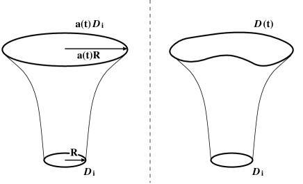
In Fig. 1 we illustrate the evolution of an initial domain ${{\cal D}_{\rm\bf i}}$ with the Hubble flow, resulting in a simple rescaling by the global scale factor $a(t)$. In a more general inhomogeneous setting the scale factor $a_{\cal D}(t)$ is defined via Eq. (1).

FIG. 1.: The evolution of an initial domain ${{\cal D}_{\rm\bf i}}$ within the Hubble flow with global scale factor $a(t)$ (left) and for a general inhomogeneous setting (right).

With $\left\langle\cdot\right\rangle_{\cal D}$ we denote spatial averaging in Eulerian space, e.g., for a spatial tensor field ${\cal A}({\mathbf{x}},t)=\{A_{ij}({\mathbf{x}},t)\}$ we simply have the Euclidean volume integral normalized by the volume of the domain:

$$\left\langle{\cal A}\right\rangle_{\cal D}=\frac{1}{V(t)}\int_{\cal D}{\rm d}^{3}x\;{\cal A}({\mathbf{x}},t).$$ (2)

For domains ${\cal D}$ with constant mass $M_{\cal D}$, as for Lagrangian defined domains, the average density is

$$\left\langle\varrho\right\rangle_{\cal D}=\frac{\left\langle\varrho({t_{\rm\bf i}})\right\rangle_{{\cal D}_{\rm\bf i}}}{a_{\cal D}^{3}}=\frac{M_{\cal D}}{a_{\cal D}^{3}{V_{\rm\bf i}}}.$$ (3)

Averaging Raychaudhuri’s equation one finds that the evolution of the scale factor $a_{\cal D}$ obeys the generalized expansion law ([2], see also Appendix A):

$$3\frac{{\ddot{a}}_{\cal D}}{a_{\cal D}}+4\pi G\left\langle\varrho\right\rangle_{\cal D}-\Lambda=Q_{\cal D},$$ (4)

with Newton’s gravitational constant $G$, the cosmological constant $\Lambda$, and the “backreaction term” $Q_{\cal D}$. For $Q_{\cal D}=0$ this equation equals one of the Friedmann equations for the scale factor $a(t)=a_{\cal D}(t)$ in an homogeneous and isotropic universe with uniform density $\varrho_{H}=\left\langle\varrho\right\rangle_{\cal D}$ ($Q_{\cal D}=0$ is a necessary, but also sufficient condition to guarantee $a_{\cal D}(t)=a(t)$). As we shall see in the next subsection the backreaction term $Q_{\cal D}$ depends on the inhomogeneities of the velocity field inside ${\cal D}$, and is generally not zero.

B Backreaction in Eulerian coordinates

Directly following from averaging Raychaudhuri’s equation we obtain the backreaction $Q_{\cal D}$ depending on the kinematical scalars, the expansion rate $\theta$, the rate of shear $\sigma$, and the rate of vorticity $\omega$ (see Appendix A):

$$Q_{\cal D}=\tfrac{2}{3}\left(\left\langle\theta^{2}\right\rangle_{\cal D}-\left\langle\theta\right\rangle_{\cal D}^{2}\right)+2\left\langle\omega^{2}-\sigma^{2}\right\rangle_{\cal D}.$$ (5)

Often it is more convenient to work with the invariants of the gradient of the velocity field as defined in Appendix B:

$$Q_{\cal D}=2\left\langle{\bf II}(v_{i,j})\right\rangle_{\cal D}-\tfrac{2}{3}\left\langle{\bf I}(v_{i,j})\right\rangle_{\cal D}^{2}.$$ (6)

The Eulerian approximation schemes are usually defined with respect to a reference frame comoving with the Hubble flow. To define such a reference frame within an inhomogeneous cosmology we have to assume that for domains ${\cal U}$ significantly larger than the averaging domain ${\cal D}$ the expansion $a(t)$ is a given solution, e.g., a solution of the Friedmann equations. Hence, using comoving coordinates we already assume that $Q_{\cal U}=0$ for very large domains ${\cal U}$. As we will see from Eq. (12) (see also Subsect. V B), this can be achieved by setting periodic boundary conditions on the inhomogeneous fields at the scale of the domain ${\cal U}$ (see also [2] for more precision). With the Hubble–parameter $H=\dot{a}/a$ we define the comoving Eulerian coordinates ${\mathbf{q}}:={\mathbf{x}}/a$ and the peculiar–velocity ${\mathbf{u}}:={\mathbf{v}}-H{\mathbf{x}}$. Using the derivative $\partial_{q_{j}}u_{i}\equiv\partial u_{i}/\partial q_{j}$ with respect to comoving coordinates we obtain for the first and second invariants:

$${\bf I}(v_{i,j}) =3H+{\bf I}(u_{i,j})=3H+\tfrac{1}{a}{\bf I}\left(\partial_{q_{j}}u_{i}\right),$$ (7)

$${\bf II}(v_{i,j}) =3H^{2}+2H{\bf I}(u_{i,j})+{\bf II}(u_{i,j})$$ (8)

$$=3H^{2}+\tfrac{2H}{a}{\bf I}\left(\partial_{q_{j}}u_{i}\right)+\tfrac{1}{a^{2}}{\bf II}\left(\partial_{q_{j}}u_{i}\right).$$ (9)

The volume–average $\left\langle{\cal A}\right\rangle_{\cal D}$ of a tensor field ${\cal A}$ can be written as a volume–average over comoving domains ${\cal D}_{q}$ defined by ${\cal D}_{q}={\cal D}(t)/a(t)$ with the comoving volume $V_{q}=V/a^{3}$:

$$\left\langle{\cal A}\right\rangle_{\cal D}=\frac{1}{V_{q}}\int_{{\cal D}_{q}}{\rm d}^{3}q\ {\cal A}.$$ (10)

The mass is conserved inside this domain ${\cal D}_{q}$. A well–known example for such comoving mass–conserving domains are the volumes used in N–body simulations.

Now, the backreaction term in comoving coordinates reads

$$Q_{\cal D}=\frac{1}{a^{2}}\left[2\ \frac{1}{V_{q}}\int_{{\cal D}_{q}}{\rm d}^{3}q\ {\bf II}\left(\partial_{q_{j}}u_{i}\right)-\right.\\ \left.-\frac{2}{3}\ \left(\frac{1}{V_{q}}\int_{{\cal D}_{q}}{\rm d}^{3}q\ {\bf I}\left(\partial_{q_{j}}u_{i}\right)\right)^{2}\right],$$ (11)

i.e., the form of $Q_{\cal D}$ is such that all Hubble terms in the velocity gradient cancel out: only inhomogeneities contribute to backreaction.

Using Eqs. (B4) and (B5) we write the backreaction as a volume–average over divergences. Hence, using the theorem of Gauss we obtain:

$$Q_{\cal D}=\frac{1}{a^{2}}\left[2\ \frac{1}{V_{q}}\int_{\partial{\cal D}_{q}}{\rm d}{\mathbf{S}}\cdot\left({\mathbf{u}}(\nabla_{q}\cdot{\mathbf{u}})-({\mathbf{u}}\cdot\nabla_{q}){\mathbf{u}}\right)-\right.\\ \left.-\frac{2}{3}\ \left(\frac{1}{V_{q}}\int_{\partial{\cal D}_{q}}{\rm d}{\mathbf{S}}\cdot{\mathbf{u}}\right)^{2}\right],$$ (12)

with the surface $\partial{\cal D}_{q}$ of the comoving domain ${\cal D}_{q}$, the surface element ${\rm d}{\mathbf{S}}$, and the comoving differential operator $\nabla_{q}$. From Eq. (12) we directly obtain $Q_{\cal D}=0$ for a domain without boundaries, i.e.  for periodic peculiar–velocity fields (see also the subsection on N–body simulations V B).

C Backreaction in Lagrangian coordinates

Let ${\mathbf{f}}(\cdot,t):{\mathbf{X}}\mapsto{\mathbf{x}}$ denote the mapping which takes the initial Lagrangian positions ${\mathbf{X}}$ of fluid elements at time ${t_{\rm\bf i}}$ to their Eulerian positions ${\mathbf{x}}$ at time $t$; i.e. ${\mathbf{x}}={\mathbf{f}}({\mathbf{X}},t)$ and ${\mathbf{X}}:={\mathbf{f}}({\mathbf{X}},{t_{\rm\bf i}})$. Then the velocity is ${\mathbf{v}}=\dot{{\mathbf{f}}}({\mathbf{X}},t)$, and the Jacobian determinant $J$ of the mapping ${\mathbf{f}}$ connects the volume elements ${\rm d}^{3}x=J{\rm d}^{3}X$.

The Lagrangian domain ${{\cal D}_{\rm\bf i}}$ is connected with the Eulerian domain by ${{\cal D}_{\rm\bf i}}={\mathbf{f}}^{-1}({\cal D},t)$, as long as ${\mathbf{f}}$ is unique. The spatial average of a tensor field ${\cal A}$ in Eulerian and Lagrangian space are related in the following way:

$$\left\langle{\cal A}\right\rangle_{\cal D}=\frac{1}{\left\langle J\right\rangle_{{\cal D}_{\rm\bf i}}}\frac{1}{{V_{\rm\bf i}}}\int_{{{\cal D}_{\rm\bf i}}}{\rm d}^{3}X\ J{\cal A}=\frac{1}{\left\langle J\right\rangle_{{\cal D}_{\rm\bf i}}}\left\langle J\;{\cal A}\right\rangle_{{\cal D}_{\rm\bf i}},$$ (13)

with

$$\left\langle J\right\rangle_{{\cal D}_{\rm\bf i}}=\frac{V}{{V_{\rm\bf i}}}=a_{\cal D}^{3}.$$ (14)

The backreaction can be expressed as a volume–average in the initial Lagrangian domain ${{\cal D}_{\rm\bf i}}$ with the velocity field ${\mathbf{v}}=\dot{{\mathbf{f}}}$ and ${\mathbf{x}}={\mathbf{f}}$:

$$Q_{\cal D}=2\ \frac{1}{\left\langle J\right\rangle_{{\cal D}_{\rm\bf i}}}\left\langle J\ {\bf II}(v_{i,j})\right\rangle_{{\cal D}_{\rm\bf i}}-\frac{2}{3}\left(\frac{1}{\left\langle J\right\rangle_{{\cal D}_{\rm\bf i}}}\left\langle J\ {\bf I}(v_{i,j})\right\rangle_{{\cal D}_{\rm\bf i}}\right)^{2}.$$ (15)

D A qualitative discussion

Eqs. (4) and (5) show that as soon as inhomogeneities are present, they are sources of the equation governing the average expansion. Upon integrating Eq. (4) we obtain ([6] used a different sign convention for $Q_{\cal D}$):

$$\frac{\dot{a}_{\cal D}^{2}+k_{\cal D}}{a_{\cal D}^{2}}-\frac{8\pi G\left\langle\varrho\right\rangle_{\cal D}}{3}-\frac{\Lambda}{3}=\frac{1}{3a_{\cal D}^{2}}\int_{{t_{\rm\bf i}}}^{t}{\rm d}t^{\prime}\ Q_{\cal D}\frac{{\rm d}}{{\rm d}s}a^{2}_{\cal D}(t^{\prime}).$$ (16)

$k_{\cal D}$ enters as an integration constant depending on the domain ${\cal D}$. With $H_{\cal D}=\dot{a}_{\cal D}/a_{\cal D}$ we define an effective Hubble–parameter, and a dimensionless “kinematical backreaction parameter”:

$$\Omega_{Q}^{\cal D}=\frac{1}{3\ a_{\cal D}^{2}H_{\cal D}^{2}}\int_{{t_{\rm\bf i}}}^{t}{\rm d}t^{\prime}\ Q_{\cal D}\ 2{\dot{a}}_{\cal D}a_{\cal D}$$ (17)

in addition to the common cosmological parameters:

$$\Omega_{m}^{\cal D}=\frac{8\pi G\left\langle\varrho\right\rangle_{\cal D}}{3H_{\cal D}^{2}},\quad\Omega_{\Lambda}^{\cal D}=\frac{\Lambda}{3H_{\cal D}^{2}},\quad\Omega_{k}^{\cal D}=-\frac{k_{D}}{a_{\cal D}^{2}H_{\cal D}^{2}}.$$ (18)

However, here, all $\Omega^{\cal D}$–parameters are domain–dependent and transformed into fluctuating fields on the domain; for $Q_{\cal D}=0$ the cosmic triangle is undistorted and the parameters acquire their global standard values. Comparing these definitions with Eq. (16) we have

$$\Omega_{m}^{\cal D}+\Omega_{\Lambda}^{\cal D}+\Omega_{k}^{\cal D}+\Omega_{Q}^{\cal D}=1.$$ (19)

In Friedmann–Lemaître cosmologies there is by definition no backreaction: $\Omega_{Q}^{\cal D}=0$. In this case a critical universe with $\Omega_{m}^{\cal D}+\Omega_{\Lambda}^{\cal D}=1$ implies $k_{\cal D}=0$, as usual. If instead $\Omega_{Q}^{\cal D}\neq 0$, and for simplicity $\Omega_{k}^{\cal D}=0$ we have an additional kinematical contribution resulting in $1=\Omega_{m}^{\cal D}+\Omega_{\Lambda}^{\cal D}+\Omega_{Q}^{\cal D}$. Contrary to the standard model, all parameters are implicit functions of spatial scale: the curvature parameter appearing as an integration constant can be different for different averaging domains ${\cal D}$, the parameter of the cosmological constant is scale–dependent through $H_{\cal D}$. As we shall see, $\Omega_{k}^{\cal D}$ can experience large changes, if initially $k_{\cal D}$ departs (even slightly) from zero.

Let us consider irrotational flows with $\omega=0$, which we may consider a good approximation until the epoch of structure formation. The averaged shear fluctuations $\left\langle\sigma^{2}\right\rangle_{\cal D}\geq 0$ and the fluctuations in the expansion rate $\left\langle\theta\right\rangle_{\cal D}^{2}-\left\langle\theta^{2}\right\rangle_{\cal D}={}\left\langle(\theta-\left\langle\theta\right\rangle_{\cal D})^{2}\right\rangle_{\cal D}\geq 0$ compete in the backreaction Eq. (5):

• $Q_{\cal D}$ is positive if the shear term dominates the expansion term. This leads to an accelerated structure formation at least in the early evolutionary stages. We then may interpret $Q_{\cal D}$ as a “kinematical dark matter”.

• $Q_{\cal D}$ is negative if the fluctuations in the expansion rate dominate. In this case $Q_{\cal D}$ acts like a (positive) “kinematical cosmological constant” leading to accelerated expansion.

Clearly such a “kinematical dark matter” will show a time dependence different from ordinary (dark) matter; also, if $Q_{\cal D}$ mimicks a cosmological term, its time–dependence will also be different than that in a $\Lambda-$cosmology.

III Quantifying the backreaction

In the last section we gave different forms of the backreaction term, and discussed qualitatively the expected consequences. Now we quantify them. Exact inhomogeneous solutions for estimating the amount of backreaction are only available for highly symmetric models like for the spherical model (Subsect. III A), and for a model with plane symmetry (Subsect. III D). In generic situations we have to rely on approximations.

A The spherical collapse

We adopt the usual assumptions. The domain of averaging ${\cal D}={\cal B}_{R}$ is a sphere with radius $R$. The velocity ${\mathbf{v}}$ inside ${\cal B}_{R}$ is only depending on the distance $r$ to the origin and always parallel to the radial unit vector $\mathbf{e}_{r}$:

$${\mathbf{v}}=v(r)\ {\mathbf{e}}_{r}.$$ (20)

Hence, we exclude rotational velocity fields. Moreover the domains stay spherical at all times. The averaged first invariant may be obtained directly using Gauss’ theorem:

$$\left\langle{\bf I}(v_{i,j})\right\rangle_{\cal D} =\frac{3}{4\pi R^{3}}\int_{\partial{\cal B}_{R}}{\rm d}{\mathbf{S}}\cdot v(r){\mathbf{e}}_{r}=3\frac{v(R)}{R},$$ (21)

whereas the averages of the second and third invariants require some basic calculations. Using Eqs. (B5), (B8) and again Gauss’ theorem leads to

$$\left\langle{\bf II}(v_{i,j})\right\rangle_{\cal D}= \frac{1}{3}\left\langle{\bf I}(v_{i,j})\right\rangle_{\cal D}^{2},$$ (22)

$$\left\langle{\bf III}(v_{i,j})\right\rangle_{\cal D}= \frac{1}{27}\left\langle{\bf I}(v_{i,j})\right\rangle_{\cal D}^{3}.$$ (23)

Combining these terms in the backreaction $Q_{{\cal B}_{R}}$ given by Eq. (6) we get for spherical symmetry

$$Q_{{\cal B}_{R}}^{\rm spherical}=0,$$ (24)

as expected from the Newtonian analogue of Birkhoff’s theorem (Newton’s “iron sphere” theorem).

B Backreaction in the Eulerian linear approximation

We calculate the backreaction in the Eulerian linear approximation using Eulerian coordinates comoving with the background Hubble flow. In this ansatz we assume that there exists a well–defined background density $\varrho_{H}$ and a global expansion factor $a(t)$ on very large scales, as already mentioned in Subsect. II B. We define the density contrast $\delta=(\varrho-\varrho_{H})/\varrho_{H}$. Additionally we assume that the growing mode of the peculiar–velocity field ${\mathbf{u}}$ is dominating, and we can neglect rotations. The time evolution of ${\mathbf{u}}({\mathbf{q}},t)$ is then proportional to the initial peculiar–velocity ${\mathbf{U}}({\mathbf{q}})={\mathbf{u}}({\mathbf{q}},{t_{\rm\bf i}})$ (see also Appendix C):

$${\mathbf{u}}({\mathbf{q}},t)=c(t){\mathbf{U}}({\mathbf{q}})\;\;.$$ (25)

With the irrotational peculiar–velocity according to Eq. (25) the invariants may be written as

$${\bf I}\left(\partial_{q_{j}}u_{i}\right) =c(t)\ {\bf I}\left(\partial_{q_{j}}U_{i}\right),$$ (26)

$${\bf II}\left(\partial_{q_{j}}u_{i}\right) =c^{2}(t)\ {\bf II}\left(\partial_{q_{j}}U_{i}\right).$$ (27)

A comoving domain is approximated by ${\cal D}_{q}={\cal D}(t)/a(t)\approx{{\cal D}_{\rm\bf i}}$ (the Eulerian approximation does not strictly conserve mass). In this approximation the volume at time $t$ is simply $V=a^{3}{V_{\rm\bf i}}$, and the backreaction in the linear approximation can be calculated using Eqs. (1), (10), and (11):

$$Q_{\cal D}^{\rm lin}=\frac{c^{2}}{a^{2}}Q_{{{\cal D}_{\rm\bf i}}}$$ (28)

with the backreaction term evaluated on the initial domain

$$Q_{{{\cal D}_{\rm\bf i}}}=2\ \left\langle{\bf II}\left(\partial_{q_{j}}U_{i}\right)\right\rangle_{{\cal D}_{\rm\bf i}}-\frac{2}{3}\ \left\langle{\bf I}\left(\partial_{q_{j}}U_{i}\right)\right\rangle_{{\cal D}_{\rm\bf i}}^{2}.$$ (29)

For an Einstein–de–Sitter background $c(t)=(t/{t_{\rm\bf i}})^{1/3}$ and $a(t)=(t/{t_{\rm\bf i}})^{2/3}$, and the backreaction term decays in proportion to the global expansion:

$$Q_{\cal D}^{\rm lin}=\left(\frac{t}{{t_{\rm\bf i}}}\right)^{-2/3}Q_{{{\cal D}_{\rm\bf i}}}.$$ (30)

Comparing the sources $Q_{\cal D}^{\rm lin}$ and $\left\langle\varrho\right\rangle_{\cal D}^{\rm lin}=\varrho_{H}({t_{\rm\bf i}})/a^{3}$ in the generalized Friedmann equation we find growth of the deviation from the standard Friedmann models, on an Einstein–de–Sitter background:

$$\frac{Q_{\cal D}^{\rm lin}}{4\pi G\left\langle\varrho\right\rangle_{\cal D}^{\rm lin}}\propto a^{2}.$$ (31)

With the function

$$h(t)=\frac{1}{a_{\cal D}^{2}}\int_{{t_{\rm\bf i}}}^{t}{\rm d}t^{\prime}\ \frac{c^{2}}{a^{2}}\ 2{\dot{a}}_{\cal D}a_{\cal D},$$ (32)

we can write the backreaction parameter $\Omega_{Q}^{\cal D}$, as given in Eq. (17), in the following form:

$$\Omega_{Q}^{\cal D}=h(t)\frac{Q_{{{\cal D}_{\rm\bf i}}}}{3\ H_{\cal D}^{2}},$$ (33)

emphasizing the analogy with a time–dependent cosmological $\Lambda$–term (see Eq. (18)).

In addition to using the linear approximation for the time evolution of the (irrotational) velocity field we assume that the comoving domain ${\cal D}_{q}$ is only weakly deformed from the initial domain ${{\cal D}_{\rm\bf i}}$. This approximation, applicable in the initial stages of structure formation, is not needed in the Lagrangian picture, where we have a definite mapping from ${{\cal D}_{\rm\bf i}}$ to ${\cal D}(t)$ as given in Subsect. II C. This illustrates that the Eulerian perturbation theory is not well–suited to calculate the backreaction of inherently mass conserving, i.e. Lagrangian, domains.

C Backreaction in the “Zel’dovich approximation”

Using the Lagrangian perturbation scheme one can construct approximate solutions which are able to trace the process of structure formation into the Eulerian nonlinear regime. As a subclass of the first–order Lagrangian perturbation series [8] the “Zel’dovich approximation” [9] is frequently used and well–studied both theoretically and numerically (see, e.g., [10], and [11] for a tutorial, and refs. therein).

As with the Eulerian perturbation approximation we assume a homogeneous–isotropic background model on very large scales, specified by the time evolution of the global expansion factor $a(t)$. The trajectory field in the “Zel’dovich approximation” is given by

$${\mathbf{f}}^{Z}({\mathbf{X}},t)=a(t)\Big{(}{\mathbf{X}}+\xi(t)\nabla_{0}\psi({\mathbf{X}})\Big{)}.$$ (34)

$\psi({\mathbf{X}})$ is the initial displacement field, $\nabla_{0}$ the gradient with respect to Lagrangian coordinates and $\xi$ a global time–dependent function (where $\xi(a)$ is given for all background models $a(t)$ in [12]).

Given the trajectory field there are two ways of implementing the approximation for the effective scale factor $a_{\cal D}$. One is based on the volume deformation of fluid elements due to the trajectory field. This results in a “passive” estimate of the time–dependence of the volume measured by the Jacobian determinant:

$$J^{Z}({\mathbf{X}},t)=a^{3}\left(1+\xi{{\bf I}_{\rm\bf i}}+\xi^{2}{{\bf II}_{\rm\bf i}}+\xi^{3}{{\bf III}_{\rm\bf i}}\right),$$ (35)

with the invariants of the initial displacement field $\psi_{|ij}$:

$${{\bf I}_{\rm\bf i}}:={\bf I}(\psi_{|ij}),\ {{\bf II}_{\rm\bf i}}:={\bf II}(\psi_{|ij}),\ {{\bf III}_{\rm\bf i}}:={\bf III}(\psi_{|ij}).$$ (36)

Now $\left\langle J^{Z}\right\rangle_{{\cal D}_{\rm\bf i}}=:(a_{\cal D}^{\rm kin})^{3}$ is given by

$$(a_{\cal D}^{\rm kin})^{3}=a^{3}\left(1+\xi\left\langle{{\bf I}_{\rm\bf i}}\right\rangle_{{\cal D}_{\rm\bf i}}+\xi^{2}\left\langle{{\bf II}_{\rm\bf i}}\right\rangle_{{\cal D}_{\rm\bf i}}+\xi^{3}\left\langle{{\bf III}_{\rm\bf i}}\right\rangle_{{\cal D}_{\rm\bf i}}\right).$$ (37)

A second possibility is to consider the dynamical backreaction equation itself and approximate the backreaction term from the velocity field ${\mathbf{v}}^{Z}=\dot{\mathbf{f}}^{Z}$ using ${\mathbf{x}}={\mathbf{f}}^{Z}$. To ease the calculations we define the functional determinant of three functions $A({\mathbf{X}})$, $B({\mathbf{X}})$, $C({\mathbf{X}})$:

$${\cal J}(A,B,C):=\frac{\partial(A,B,C)}{\partial(X_{1},X_{2},X_{3})}=\epsilon_{ijk}A_{|i}B_{|j}C_{|k}.$$ (38)

(For example: the Jacobian determinant of the Lagrangian mapping ${\mathbf{f}}=(f_{1},f_{2},f_{3})$ reads $J={\cal J}(f_{1},f_{2},f_{3})$.) Now we express the invariants of the velocity field ${\mathbf{v}}=\dot{{\mathbf{f}}}$ in terms of functional determinants,

$${\bf I}(v_{i,j}) =\tfrac{1}{2J}\epsilon_{ijk}{\cal J}(\dot{f}_{i},f_{j},f_{k}),$$ (39)

$${\bf II}(v_{i,j}) =\tfrac{1}{2J}\epsilon_{ijk}{\cal J}(\dot{f}_{i},\dot{f}_{j},f_{k}),$$ (40)

which may be verified using

$$v_{i,j}=\tfrac{1}{2J}\ \epsilon_{jkl}{\cal J}(\dot{f}_{i},f_{k},f_{l}).$$ (41)

Inserting the approximation Eq. (34) we get with $b(t)=a(t)\xi(t)$:

$${\cal J}(\dot{f}^{Z}_{i},f^{Z}_{j},f^{Z}_{k}) =\dot{a}a^{2}\ {\cal J}(X_{i},X_{j},X_{k})+\dot{b}b^{2}\ {\cal J}(\psi_{|i},\psi_{|j},\psi_{|k})$$ (42)

$$\quad+(2a\dot{a}b+a^{2}\dot{b})\ {\cal J}(X_{i},X_{j},\psi_{|k})$$ (43)

$$\quad+(2a\dot{b}b+\dot{a}b^{2})\ {\cal J}(X_{i},\psi_{|j},\psi_{|k}),$$ (44)

$${\cal J}(\dot{f}^{Z}_{i},\dot{f}^{Z}_{j},f^{Z}_{k}) =\dot{a}^{2}a\ {\cal J}(X_{i},X_{j},X_{k})+\dot{b}^{2}b\ {\cal J}(\psi_{|i},\psi_{|j},\psi_{|k})$$ (45)

$$\quad+(2\dot{a}a\dot{b}+\dot{a}^{2}b)\ {\cal J}(X_{i},X_{j},\psi_{|k})$$ (46)

$$\quad+(2\dot{a}\dot{b}b+a\dot{b}^{2})\ {\cal J}(X_{i},\psi_{|j},\psi_{|k}).$$ (47)

Again, these functional determinants are related to the invariants of the initial displacement field $\psi_{|ij}$ (see Eq. (36)):

$$\epsilon_{ijk}{\cal J}(X_{i},X_{j},X_{k}) =6$$ (48)

$$\epsilon_{ijk}{\cal J}(X_{i},X_{j},\psi_{|k}) =2{{\bf I}_{\rm\bf i}},$$ (49)

$$\epsilon_{ijk}{\cal J}(X_{i},\psi_{|j},\psi_{|k}) =2{{\bf II}_{\rm\bf i}},$$ (50)

$$\epsilon_{ijk}{\cal J}(\psi_{|i},\psi_{|j},\psi_{|k}) =6{{\bf III}_{\rm\bf i}}.$$ (51)

Hence, with $K:=\dot{\xi}/\xi$ and $H:=\dot{a}/a$,

$$\frac{1}{a^{3}}\ \epsilon_{ijk}{\cal J}(\dot{f}^{Z}_{i},f^{Z}_{j},f^{Z}_{k})= 6H+2\ {{\bf I}_{\rm\bf i}}\ \xi(3H+K)$$ (52)

$$+2\ {{\bf II}_{\rm\bf i}}\ \xi^{2}(3H+2K)$$ (53)

$$+6\ {{\bf III}_{\rm\bf i}}\ \xi^{3}(H+K),$$ (54)

$$\frac{1}{a^{3}}\ \epsilon_{ijk}{\cal J}(\dot{f}^{Z}_{i},\dot{f}^{Z}_{j},f^{Z}_{k})= 6H^{2}+2\ {{\bf I}_{\rm\bf i}}\ \xi(3H^{2}+2HK)$$ (55)

$$+2\ {{\bf II}_{\rm\bf i}}\ \xi^{2}(3H^{2}+4HK+K^{2})$$ (56)

$$+6\ {{\bf III}_{\rm\bf i}}\ \xi^{3}(H^{2}+2HK+K^{2}).$$ (57)

Using Eqs. (52, 55) inserted into Eq. (40) we can calculate the invariants of $v_{i,j}$ as they appear in Eq. (15). Combined with Eq. (37) the backreaction term separates into its time–evolution given by $\xi(t)$ and the spatial dependence on the initial displacement field given by averages over the invariants ${{\bf I}_{\rm\bf i}},{{\bf II}_{\rm\bf i}},{{\bf III}_{\rm\bf i}}$:

$$Q^{Z}_{\cal D}=\frac{\dot{\xi}^{2}}{\left(1+\xi\left\langle{{\bf I}_{\rm\bf i}}\right\rangle_{{\cal D}_{\rm\bf i}}+\xi^{2}\left\langle{{\bf II}_{\rm\bf i}}\right\rangle_{{\cal D}_{\rm\bf i}}+\xi^{3}\left\langle{{\bf III}_{\rm\bf i}}\right\rangle_{{\cal D}_{\rm\bf i}}\right)^{2}}\times\\[4.30554pt] \Big{[}\left(2\left\langle{{\bf II}_{\rm\bf i}}\right\rangle_{{\cal D}_{\rm\bf i}}-\tfrac{2}{3}\left\langle{{\bf I}_{\rm\bf i}}\right\rangle_{{\cal D}_{\rm\bf i}}^{2}\right)+\xi\left(6\left\langle{{\bf III}_{\rm\bf i}}\right\rangle_{{\cal D}_{\rm\bf i}}-\tfrac{2}{3}\left\langle{{\bf I}_{\rm\bf i}}\right\rangle_{{\cal D}_{\rm\bf i}}\left\langle{{\bf II}_{\rm\bf i}}\right\rangle_{{\cal D}_{\rm\bf i}}\right)\\ +\xi^{2}\left(2\left\langle{{\bf I}_{\rm\bf i}}\right\rangle_{{\cal D}_{\rm\bf i}}\left\langle{{\bf III}_{\rm\bf i}}\right\rangle_{{\cal D}_{\rm\bf i}}-\tfrac{2}{3}\left\langle{{\bf II}_{\rm\bf i}}\right\rangle_{{\cal D}_{\rm\bf i}}^{2}\right)\Big{]}.$$ (58)

The numerator of the first term is global and corresponds to the linear damping factor; in an Einstein–de–Sitter universe $\dot{\xi}^{2}\propto a^{-1}$. The denominator of the first term is a volume effect, whereas the second term in brackets features the initial backreaction as a leading term.

In the following we will stick to an Einstein–de–Sitter background with $a(t)=(t/{t_{\rm\bf i}})^{2/3}$ and $\nabla_{0}\psi({\mathbf{X}})=3/2{\mathbf{U}}({\mathbf{X}}){t_{\rm\bf i}}$ [9, 8]. $\xi(t)$ equals $a(t)-1$, since ${\mathbf{f}}({\mathbf{X}},{t_{\rm\bf i}})={\mathbf{X}}$ with $a({t_{\rm\bf i}})=1$.

In the early stages of structure formation with $\xi(t)\ll 1$ we get

$$Q^{Z}_{\cal D}\approx\left(\frac{t}{{t_{\rm\bf i}}}\right)^{-\frac{2}{3}}\ Q_{{\cal D}_{\rm\bf i}},$$ (59)

identical to the early evolution in the Eulerian linear approximation Eq. (30). Moreover, for $t={t_{\rm\bf i}}$ we have $Q^{Z}_{\cal D}=Q_{{\cal D}_{\rm\bf i}}$ consistent with Eq. (4). For late times and positive invariants $\left\langle{{\bf I}_{\rm\bf i}}\right\rangle_{{\cal D}_{\rm\bf i}},\left\langle{{\bf II}_{\rm\bf i}}\right\rangle_{{\cal D}_{\rm\bf i}},\left\langle{{\bf III}_{\rm\bf i}}\right\rangle_{{\cal D}_{\rm\bf i}}>0$ the dominating contribution is proportional to $\dot{\xi}^{2}/\xi^{4}$ and $Q^{Z}_{\cal D}$ decays. However, for negative invariants, the $Q^{Z}_{\cal D}$ term diverges at some time when $1+\xi\left\langle{{\bf I}_{\rm\bf i}}\right\rangle_{{\cal D}_{\rm\bf i}}+\xi^{2}\left\langle{{\bf II}_{\rm\bf i}}\right\rangle_{{\cal D}_{\rm\bf i}}+\xi^{3}\left\langle{{\bf III}_{\rm\bf i}}\right\rangle_{{\cal D}_{\rm\bf i}}$ passes through zero. This is the signature of pancake–collapse on the scale of the domain. A variety of complex phenomena may be expected for averaged invariants with different signs.

D An exact reference solution: the plane collapse

The “Zel’dovich approximation” is an exact three–dimensional solution to the Newtonian dynamics of self–gravitating dust–matter for initial conditions with ${\bf II}(\psi_{|ij})=0={\bf III}(\psi_{|ij})$ at each point [13]. This “locally one–dimensional” class of motions contains as a sub case the globally plane–symmetric solution [14]. Eq. (58) reduces to

$$Q^{\rm plane}_{\cal D}=-\frac{2}{3}\ \frac{\dot{\xi}^{2}\left\langle{{\bf I}_{\rm\bf i}}\right\rangle_{{\cal D}_{\rm\bf i}}^{2}}{(1+\xi\left\langle{{\bf I}_{\rm\bf i}}\right\rangle_{{\cal D}_{\rm\bf i}})^{2}}.$$ (60)

We compare the two exact solutions, the plane and the spherical model in Subsect. IV A 2. For negative $\left\langle{{\bf I}_{\rm\bf i}}\right\rangle_{{\cal D}_{\rm\bf i}}$, corresponding to over–dense regions (Eq. (C13)), $Q^{\rm plane}_{\cal D}$ is diverging at some time when $1+\xi(t)\left\langle{{\bf I}_{\rm\bf i}}\right\rangle_{{\cal D}_{\rm\bf i}}$ approaches zero. Our special initial conditions imply a one–dimensional symmetry of inhomogeneities, and the diverging $Q^{\rm plane}_{\cal D}$ is supposed to mimick the highly anisotropic pancake collapse in the three–dimensional situation.

E Zel’dovich’s approximation and the spherical collapse

In the situation of a spherical collapse (Subsect. III A) we have seen that the averaged invariants obey relations resulting in

$$\left\langle{{\bf II}_{\rm\bf i}}\right\rangle_{{\cal B}_{R}}=\frac{1}{3}\left\langle{{\bf I}_{\rm\bf i}}\right\rangle_{{\cal B}_{R}}^{2},\quad\text{and}\quad\left\langle{{\bf III}_{\rm\bf i}}\right\rangle_{{\cal B}_{R}}=\frac{1}{27}\left\langle{{\bf I}_{\rm\bf i}}\right\rangle_{{\cal B}_{R}}^{3}.$$ (61)

Inserting this into the backreaction term Eq. (58) we obtain $Q^{Z}_{{\cal B}_{R}}=0=Q^{\rm spherical}_{{\cal B}_{R}}$. Hence, the “Zel’dovich approximation” together with the generalized Friedmann equation results also in an exact solution for the evolution of the effective scale factor $a_{\cal D}$, if restricted to the special initial conditions ${\mathbf{U}}=U(r)\ \mathbf{e}_{r}$.

IV The evolution of cosmological parameters

The backreaction term itself decays in the linear approximation and also at early stages in the “Zel’dovich approximation”. However, to quantify the deviations from the behavior of the scale factor in the standard model, the different strength of the sources in the generalized Friedmann equation has to be compared. As already noted in the Eulerian linear approximation, the dimensionless contribution to backreaction (as compared to the global mean density) grows.

A Evolution of the scale factor $a_{\cal D}$

We proceed as follows. We use the backreaction terms calculated in the preceding sections, insert them into the generalized expansion law Eq. (4), and solve for $a_{\cal D}(t)$. We determine generic initial conditions numerically as summarized in Appendix C.

Assuming an Einstein–de–Sitter background we subtract a standard Friedmann equation $3\tfrac{{\ddot{a}}}{a}+4\pi G\varrho_{H}=0$, from Eq. (4), use $\varrho_{H}=\tfrac{3H^{2}}{8\pi G}$ and obtain the following differential equation for $a_{\cal D}(t)$:

$$3\left(\frac{{\ddot{a}_{\cal D}}}{a_{\cal D}}-\frac{{\ddot{a}}}{a}\right)+\frac{3}{2}\left(\frac{{\dot{a}}}{a}\right)^{2}\left\langle\delta\right\rangle_{\cal D}=Q_{\cal D}\;\;,$$ (62)

with $\left\langle\delta\right\rangle_{\cal D}=(\left\langle\varrho\right\rangle_{\cal D}-\varrho_{H})/\varrho_{H}$ specifying the averaged density contrast in ${\cal D}$. For $Q_{\cal D}=0$ and $\left\langle\delta\right\rangle_{\cal D}=0$ this equation simply states that the time evolution of a domain follows the global expansion, $a_{\cal D}(t)=a(t)$. The averaged density contrast is related to the averaged first invariant $\left\langle{{\bf I}_{\rm\bf i}}\right\rangle_{{\cal D}_{\rm\bf i}}$ as given in Eq. (C13). For $Q_{\cal D}=0$ and $1+\left\langle\delta\right\rangle_{\cal D}=\frac{\left\langle\varrho\right\rangle_{\cal D}a^{3}}{\varrho_{H}a_{\cal D}^{3}}$ the evolution of $a_{\cal D}$ is still of Friedmann type, but with a mass different from the homogeneous background mass. An important sub case with $Q_{\cal D}=0$ and $\left\langle\delta\right\rangle_{\cal D}\neq 0$ is the well–known spherical top–hat model [15]. In Eq. (62) there are two sources determining the deviations from the Friedmann acceleration, the over/under–density and the backreaction term: the evolution of a spatial domain is triggered by an over/under–density and velocity fluctuations. Eq. (62) can be interpreted as a natural generalization of the top–hat model. Engineer et al.  [16] also incorporate shear and angular momentum to formulate and study generalizations of the spherical top–hat model. Their emphasis, however, is focussed on the improvement of the virialization and other clustering arguments.

To solve this differential equation we specify the initial conditions according to the background model:

$$a(t)=\left(\frac{t}{{t_{\rm\bf i}}}\right)^{2/3}\text{ with }{t_{\rm\bf i}}=\frac{2}{3H_{0}(1+{z_{\rm\bf i}})^{3/2}}.$$ (63)

$H_{0}$ is the present value of the Hubble–parameter of the background model, and ${z_{\rm\bf i}}$ the redshift where we start our calculations. With $H_{0}=50{\rm km\ s}^{-1}{\rm Mpc}^{-1}$ and ${z_{\rm\bf i}}=200$ the initial starting time is ${t_{\rm\bf i}}=4.6\ 10^{-3}{\rm Gy}$. The scale factor $a_{\cal D}$ of the domain is chosen to match the background scale factor $a$ at time ${t_{\rm\bf i}}$:

$$a_{\cal D}({t_{\rm\bf i}})=a({t_{\rm\bf i}})=1.$$ (64)

We stop at the present epoch $z_{0}=0$ and $t_{0}=13{\rm Gy}$, with $a(t_{0})=201$. Following directly from Eq. (A3), ${\dot{a}_{\cal D}}$ is given by

$${\dot{a}_{\cal D}}({t_{\rm\bf i}})={\dot{a}}({t_{\rm\bf i}})\left(1+\tfrac{1}{3}\left\langle{{\bf I}_{\rm\bf i}}\right\rangle_{{\cal D}_{\rm\bf i}}\right)=\frac{2}{3{t_{\rm\bf i}}}\left(1+\tfrac{1}{3}\left\langle{{\bf I}_{\rm\bf i}}\right\rangle_{{\cal D}_{\rm\bf i}}\right).$$ (65)

Often ${\dot{a}_{\cal D}}({t_{\rm\bf i}})={\dot{a}}({t_{\rm\bf i}})$ is used to specify the initial conditions for the investigation of collapse times within the spherical model. Numerical tests showed that for these inconsistent initial conditions the collapse is delayed as already discussed by Bartelmann et al. [17].

For the numerical integration we used the Runge–Kutta routine given in Press et al. [18]. Identical results were obtained with the NDSolve routine of Mathematica.

1 Initial conditions

In Sect. III we expressed the term $Q_{\cal D}$ using globally given time–functions $a(t)$, $\xi(t)$, and using the volume–averaged invariants $\left\langle{{\bf I}_{\rm\bf i}}\right\rangle_{{\cal D}_{\rm\bf i}}$, $\left\langle{{\bf II}_{\rm\bf i}}\right\rangle_{{\cal D}_{\rm\bf i}}$, $\left\langle{{\bf III}_{\rm\bf i}}\right\rangle_{{\cal D}_{\rm\bf i}}$ for the initial domain ${{\cal D}_{\rm\bf i}}$. The relation of these volume–averaged invariants to the initial power spectrum is discussed in Appendix C in detail using the linear approximation. We determine the initial values of the averaged invariants for a spherical initial domain ${\cal B}_{R}$ of radius $R$, assuming a Gaussian initial density field, with a Cold–Dark–Matter (CDM) power spectrum.

The ensemble mean ${\mathbb{E}}$, i.e.  the expectation value, of the volume–averaged invariants vanishes in conformity with our global set–up:

$${\mathbb{E}}\left[\left\langle{{\bf I}_{\rm\bf i}}\right\rangle_{{\cal B}_{R}}\right]={\mathbb{E}}\left[\left\langle{{\bf II}_{\rm\bf i}}\right\rangle_{{\cal B}_{R}}\right]={\mathbb{E}}\left[\left\langle{{\bf III}_{\rm\bf i}}\right\rangle_{{\cal B}_{R}}\right]=0.$$ (66)

However, for a specific domain, any of the volume–averaged invariants may be positive or negative. These invariants fluctuate with the variance, e.g., $\sigma_{{\bf I}}^{2}(R)={\mathbb{E}}\left[\left\langle{{\bf I}_{\rm\bf i}}\right\rangle_{{\cal B}_{R}}^{2}\right]$. We consider one–$\sigma$ fluctuations, e.g. $\left\langle{{\bf I}_{\rm\bf i}}\right\rangle_{{\cal B}_{R}}=\pm\sigma_{{\bf I}}(R)$, and also two– and three–$\sigma$ fluctuations of the averaged invariants in our calculations of the time evolution of $a_{\cal D}(t)$. Clearly, these fluctuations depend on the shape of the power spectrum and the radius of the initial domain. In Table. I we give the values for spherical domains of different sizes, as calculated in Appendix C for the standard CDM model. Moreover, we could show that the volume–averaged invariants are uncorrelated for a Gaussian initial density field, and may be specified independently.

TABLE I.: The mean mass fluctuations $\sigma_{{\bf I}}(R)$, $\sigma_{{\bf II}}(R)$, and $\sigma_{{\bf III}}(R)$ for an initial domain of radius $R$ are given, calculated using the CDM power spectrum. To make these numbers more accessible, also the linearly extrapolated mean fluctuations $a(t_{0})\sigma_{{\bf I}}(R)$ for a domain with scaled radius $a(t_{0})R$ at present time are given (compare Fig. 1).

$aR$ [Mpc]	5	16	50	100	251	503	1005
$a\sigma_{{\bf I}}$	2.6	1.0	0.27	0.1	0.025	0.0068	0.0019
$R$ [Mpc]	0.025	0.08	0.25	0.5	1.25	2.5	5
$\sigma_{{\bf I}}$ $\times 10^{3}$	13	5.0	1.4	0.51	0.13	0.03	0.01
$\sigma_{{\bf II}}$ $\times 10^{6}$	90	20	2	0.4	0.07	0.02	0.004
$\sigma_{{\bf III}}$ $\times 10^{12}$	81000	4600	100	5	0.08	0.001	0.00004

2 The plane and spherical collapse

We calculate the evolution of the scale factor $a_{\cal D}(t)$ according to Eq. (62) using the backreaction term calculated within the “Zel’dovich approximation” (58) with $a(t)=(t/{t_{\rm\bf i}})^{2/3}$ and $\xi(t)=a(t)-1$.

First we consider initial conditions with $\left\langle{{\bf II}_{\rm\bf i}}\right\rangle_{{\cal B}_{R}}=0=\left\langle{{\bf III}_{\rm\bf i}}\right\rangle_{{\cal B}_{R}}$ and $\left\langle{{\bf I}_{\rm\bf i}}\right\rangle_{{\cal B}_{R}}\neq 0$, the plane collapse solution Eq. (60). We choose $\left\langle{{\bf I}_{\rm\bf i}}\right\rangle_{{\cal B}_{R}}\neq 0$ comparable to the mean fluctuations $\sigma_{{\bf I}}(R)$ in initially spherical domains with radius $R\in\{0.025,0.08,0.25,0.5\}$Mpc (a scaled, present–day radius of $a(t_{0})R\in\{5,16,50,100\}$Mpc) as given in Table I. From Fig. 2 it can be seen that the evolution of the scale factor $a_{\cal D}(t)$ may significantly differ from the background expansion $a(t)$ for an initial domain radius $R=0.25$Mpc (a scaled radius of $a(t_{0})R=50$Mpc). For small domains with larger $\left\langle{{\bf I}_{\rm\bf i}}\right\rangle_{{\cal B}_{R}}$ the effect is more pronounced. For negative $\left\langle{{\bf I}_{\rm\bf i}}\right\rangle_{{\cal B}_{R}}$ (an over–dense region) the region shows a pancake collapse with $Q_{\cal D}\rightarrow\infty$, as a result of the one–dimensional symmetry in the initial conditions. For initial domains with $R\geq 2.5$Mpc (a scaled radius of $a(t_{0})R\geq 503$Mpc) the value of $\left\langle{{\bf I}_{\rm\bf i}}\right\rangle_{{\cal B}_{R}}$ is typically so small that the $a_{\cal D}(t)$ closely follows the Friedmann solution until present. In the following we compare the two inhomogeneous exact solutions, the plane and spherical collapse, disentangling the influence of the backreaction term $Q_{\cal D}$ from the influence of the over–density.

FIG. 2.: The curves show the scale factor $a_{\cal D}(t)$ in the spherical collapse (dotted) and the plane collapse (solid) for $\left\langle{{\bf I}_{\rm\bf i}}\right\rangle_{{\cal B}_{R}}\in\{-13,-5.0,-1.4,-0.51,0.51,1.4,5.0,13\}\times 10^{-3}$, bending up successively. These values correspond to one–$\sigma$ fluctuations of spherical domains with a scaled radius of $a(t_{0})R\in\{5,16,50,100\}$Mpc (see Table I). The homogeneous background solution is given as the dashed line.

As shown in Subsect. III A, the backreaction $Q_{\cal D}$ is zero for a spherical domain with spherical symmetric velocity field. However, this domain may still be over– or under–dense compared to the background density. The evolution of the scale factor of this domain is then determined by Eq. (62) with $Q_{\cal D}=0$ and $\left\langle\delta\right\rangle_{\cal D}\neq 0$, which is exactly the spherical collapse model [15].

In Fig. 2 we compare the evolution of $a_{\cal D}(t)$ in this spherical collapse model with the plane collapse model. For $|\left\langle{{\bf I}_{\rm\bf i}}\right\rangle_{{\cal B}_{R}}|=1.4$, typical for domains with a scaled radius of $a(t_{0})R=50$Mpc, both models give nearly the same evolution. However for increasingly over-dense regions (negative $\left\langle{{\bf I}_{\rm\bf i}}\right\rangle_{{\cal B}_{R}}$) the plane model decouples and collapses significantly earlier than the spherical model. Also the expansion of under–dense regions is slowing down in the plane compared with the spherical collapse model. These results are in agreement with earlier results on collapse–times of structure in Lagrangian perturbation schemes [19, 20, 17, 21, 22].

3 Generic initial data

The behavior of $a_{\cal D}(t)$ becomes more interesting if we consider the other two invariants, going beyond the exact solutions. For simplicity we choose $\left\langle{{\bf I}_{\rm\bf i}}\right\rangle_{{\cal B}_{R}}=0$ corresponding to a domain with $\left\langle\delta\right\rangle_{{\cal B}_{R}}=0$ matching the background density at initial time ${t_{\rm\bf i}}$. The effect of a nonzero second invariant $\left\langle{{\bf II}_{\rm\bf i}}\right\rangle_{{\cal B}_{R}}\neq 0$ is visible in Fig. 3. Already in a domain with an initial radius of $R=0.25$Mpc (a scaled radius of $a(t_{0})R\approx 50$Mpc) the $a_{\cal D}$ may deviate from the Friedmann solution. Although we consider volumes with no initial over–density and with only one–$\sigma$ fluctuations of $\left\langle{{\bf II}_{\rm\bf i}}\right\rangle_{{\cal B}_{R}}$, domains of a current size of $a(t_{0})R\approx 16$Mpc may collapse.

FIG. 3.: The curves shown are the evolution of the scale factor $a_{\cal D}(t)$ for initial conditions with $\left\langle{{\bf I}_{\rm\bf i}}\right\rangle_{{\cal B}_{R}}=0=\left\langle{{\bf III}_{\rm\bf i}}\right\rangle_{{\cal B}_{R}}$ and $\left\langle{{\bf II}_{\rm\bf i}}\right\rangle_{{\cal B}_{R}}\in\{-90,-20,-2,2,20,90\}\times 10^{-6}$ shown as the solid lines bending up successively. These values correspond to one–$\sigma$ fluctuations of spherical domains with a scaled radius of {5,16,50}Mpc (see Table I). The homogeneous background solution is given as the dashed line.

The influence of the third invariant on the evolution of the scale factor is small (in the temporal range considered) compared to the influence of $\left\langle{{\bf I}_{\rm\bf i}}\right\rangle_{{\cal B}_{R}}$ and $\left\langle{{\bf II}_{\rm\bf i}}\right\rangle_{{\cal B}_{R}}$. To illustrate this we consider domains with $\left\langle{{\bf I}_{\rm\bf i}}\right\rangle_{{\cal B}_{R}}=0=\left\langle{{\bf II}_{\rm\bf i}}\right\rangle_{{\cal B}_{R}}$ and one–$\sigma$ fluctuations of $\left\langle{{\bf III}_{\rm\bf i}}\right\rangle_{{\cal B}_{R}}$. For an initial domain of radius $0.025$Mpc (a scaled radius of 5Mpc) a significant influence is visible (Fig. 4). Already for an initial domain of radius $0.08$Mpc (a scaled radius of 16Mpc) the influence is small, becoming negligible on larger scales.

FIG. 4.: The evolution of the scale factor $a_{\cal D}(t)$ for initial conditions with $\left\langle{{\bf I}_{\rm\bf i}}\right\rangle_{{\cal B}_{R}}=0=\left\langle{{\bf II}_{\rm\bf i}}\right\rangle_{{\cal B}_{R}}$ and $\left\langle{{\bf III}_{\rm\bf i}}\right\rangle_{{\cal B}_{R}}\in\{-81,-4.6,4.6,81\}\times 10^{-15}$ shown as the solid lines bending up successively. These values correspond to one–$\sigma$ fluctuations of spherical domains with a present day scaled radius of 5 and 16Mpc (see Table I). The homogeneous background solution is given as the dashed line.

Up to now we only considered domains with initial conditions chosen as one–$\sigma$ fluctuations in either $\left\langle{{\bf I}_{\rm\bf i}}\right\rangle_{{\cal B}_{R}}$, $\left\langle{{\bf II}_{\rm\bf i}}\right\rangle_{{\cal B}_{R}}$, or $\left\langle{{\bf III}_{\rm\bf i}}\right\rangle_{{\cal B}_{R}}$. As can be seen from Fig. 5 the evolution of the scale factor is strongly depending on the initial conditions, even for a domain with initial radius 0.25Mpc (a scaled radius of 50Mpc), if we also consider two–$\sigma$ or three–$\sigma$ fluctuations. Such a domain may even collapse.

FIG. 5.: The evolution of the scale factor $a_{\cal D}(t)$ for spherical domains with a scaled radius of 50Mpc. We considered one–$\sigma$ (dotted line), two–$\sigma$ (short dashed line), and three–$\sigma$ (long dashed line) fluctuations of $\left\langle{{\bf I}_{\rm\bf i}}\right\rangle_{{\cal B}_{R}}$, $\left\langle{{\bf II}_{\rm\bf i}}\right\rangle_{{\cal B}_{R}}$, and $\left\langle{{\bf III}_{\rm\bf i}}\right\rangle_{{\cal B}_{R}}$ (see Table I). The evolution shown are obtained for $\left\langle{{\bf I}_{\rm\bf i}}\right\rangle_{{\cal B}_{R}},\left\langle{{\bf II}_{\rm\bf i}}\right\rangle_{{\cal B}_{R}},\left\langle{{\bf III}_{\rm\bf i}}\right\rangle_{{\cal B}_{R}}<0$ (over–dense) and $\left\langle{{\bf I}_{\rm\bf i}}\right\rangle_{{\cal B}_{R}},\left\langle{{\bf II}_{\rm\bf i}}\right\rangle_{{\cal B}_{R}},\left\langle{{\bf III}_{\rm\bf i}}\right\rangle_{{\cal B}_{R}}>0$ (under–dense). The homogeneous background solution is given by the solid line.

Using the present approach we already assume that the backreaction term gives a negligible contribution on the largest scale. Hence, for increasing size of the initial domain the evolution of the scale factor goes more and more conform with the Friedmann evolution (see Fig. 6). Still for a domain with a scaled radius of 100Mpc deviations of the order of 15% in the scale factor at present time may be obtained for initial fluctuations at the three-$\sigma$ level. The scaled volume of such a domain corresponds to a cube with $\approx 160$Mpc side length – still a typical volume used in $N$–body simulations. For domains with a scaled radius of 250Mpc ($\approx 400$Mpc side length of a cube) we may get deviations of the order of 3% from the Friedmann value $a(t_{0})$, for initial fluctuations at the three-$\sigma$ level. In Sects. IV A 5 and IV B we will see that the influence on the domains’ Hubble– and deceleration–parameter as well as on its density parameters is more pronounced, because these parameters invoke the time–derivatives of $a_{\cal D}(t)$.

FIG. 6.: The evolution of the scale factor $a_{\cal D}(t)$ for spherical domains with a scaled radius of 100Mpc (upper plot) and 250Mpc (lower plot). The same conventions as in Fig. 5 are used.

4 Comparison with the Eulerian linear approximation

Using the backreaction term (30) in the generalized evolution equation (62) we calculate the time evolution of $a_{\cal D}^{\rm lin}(t)$ in the Eulerian linear approximation. In Fig. 7 we compare the evolution of the scale factor in the “Zel’dovich approximation” with the evolution in the Eulerian linear approximation. Even though we consider three–$\sigma$ initial conditions, the evolution of under–dense domains with a scaled radius larger than 50Mpc is described nearly perfectly by the Eulerian linear approximation. For over–dense domains the concordance with the “Zel’dovich approximation” is reasonable for domains with a scaled radius larger than 100Mpc. The Eulerian linear approximation fails to describe a collapsing domain. However, we see that the backreaction term is not only important for small domains, where the nonlinear evolution plays a dominant role, but also for large domains within the realm of linear theory. We emphasize that these remarks are concerned with the average performance; linear theory does not predict correctly where mass is moved, as cross–correlation tests with Lagrangian perturbative schemes and N–body runs (even if smoothed on larger scales) have shown [23].

FIG. 7.: The evolution of the scale factor $a_{\cal D}(t)$ for three–$\sigma$ initial conditions as already used in Fig. 6. The curves are for over–dense domains with a scaled radius of 50, 100, 250Mpc, and under–dense domains with a scaled radius of 250, 100, 50Mpc, bending up successively. The evolution of $a_{\cal D}^{Z}$ is given by the solid lines, the evolution of $a_{\cal D}^{\rm lin}$ by the dotted lines. The evolution according to the Friedmann solution is given by the dashed line.

5 Evolution of the Hubble– and deceleration–parameter

Not only the evolution of the scale factor itself is interesting, but also the derived quantities like the Hubble–parameter $H_{\cal D}={\dot{a}}_{\cal D}/a_{\cal D}$ and the deceleration parameter $q_{\cal D}=-\frac{{\ddot{a}}_{\cal D}/a_{\cal D}}{H_{\cal D}^{2}}$ are of specific interest.

From Fig. 8 we see that at present a 20% variability of the Hubble–parameter $H_{\cal D}$ is quite common in a domain with a scaled radius of 100Mpc (three–$\sigma$ initial conditions). For a domain with a scaled radius of 250Mpc still 3% variation is possible. This agrees well with the results obtained by Wu et al. [24] for a regional low–density universe (see also [25], [26], and refs. therein).

FIG. 8.: The evolution of the Hubble–parameter $H_{\cal D}(t)$ for a spherical domain with a scaled radius of 100Mpc. Over–dense domains show a smaller $H_{\cal D}$ than in an Einstein–de–Sitter universe (solid line), under–dense an increased $H_{\cal D}$. The same conventions as in Fig. 5 are used.

The effect becomes more pronounced if one considers the deceleration parameter $q_{\cal D}$, as shown in Fig. 9. In a domain with a scaled radius of 100Mpc the $q_{\cal D}$ may show a present day value of more than 200% different from the background Einstein–de–Sitter universe. Even for a domain with a scaled radius of 250Mpc a difference larger than 15% is possible.

FIG. 9.: The evolution of the deceleration parameter $q_{\cal D}(t)$ for a spherical domain with a scaled radius of 100Mpc. Over–dense domains show an increased $q_{\cal D}$ compared to an Einstein–de–Sitter universe (solid line), under–dense domains a decreased $q_{\cal D}$. The same conventions as in Fig. 5 apply.

Consider the situation that our regional Universe may be an under–dense portion (say, resulting from an under–density at 0.5–$\sigma$ on the scale of the considered portion). Then, we may well live in a shear–dominated part of the Universe: many low–amplitude anisotropic structures surround us which are compatible with a regional under–density, but would suggest a dominance by shear fluctuations (say, resulting from a positive second invariant in the initial conditions at three–$\sigma$). Such domains with density–contrast and velocity fluctuations working “against” each other may show a qualitative change in their evolution as illustrated in Fig. 10: an initially under–dense region, however, dominated by shear fluctuations may show a deceleration.

FIG. 10.: The evolution of the regional deceleration parameter $q_{\cal D}(t)$ for a spherical domain with a scaled radius of 100Mpc. The initial conditions are chosen as 0.5–$\sigma$ for $\left\langle{{\bf I}_{\rm\bf i}}\right\rangle_{{\cal B}_{R}}$ and three–$\sigma$ for both $\left\langle{{\bf II}_{\rm\bf i}}\right\rangle_{{\cal B}_{R}}$ and $\left\langle{{\bf III}_{\rm\bf i}}\right\rangle_{{\cal B}_{R}}$ with the opposite sign of $\left\langle{{\bf I}_{\rm\bf i}}\right\rangle_{{\cal B}_{R}}$. The initially accelerating, i.e.  under–dense region ($\left\langle{{\bf I}_{\rm\bf i}}\right\rangle_{{\cal B}_{R}}>0$) finally decelerates (dotted line) whereas the initially over–dense region (dashed line) shows an accelerated expansion at late times.

B Evolution of the density parameters

Now we turn our attention to the domain–dependent “cosmological parameters” defined in Subsect. II D. Knowing the time evolution of $a_{\cal D}$ for given initial conditions we can calculate the time evolution of $\Omega_{m}^{\cal D}$, $\Omega_{k}^{\cal D}$, and $\Omega_{Q}^{\cal D}$. Again we assume that the global evolution follows an Einstein–de–Sitter model with $\Omega_{\Lambda}=0=\Omega_{\Lambda}^{\cal D}$ and on the largest scale $\Omega_{k}=0$. However, as shown below, for finite domains ${\cal D}$ the time evolution of the “cosmological parameters” can substantially differ from the Friedmann evolution even for small, seemingly negligible backreaction term. We have for the density and “curvature” parameter:

$$\Omega_{m}^{\cal D}(t)= \frac{H^{2}({t_{\rm\bf i}})\ (1-\left\langle{{\bf I}_{\rm\bf i}}\right\rangle_{{\cal D}_{\rm\bf i}})}{{\dot{a}}_{\cal D}(t)^{2}a_{\cal D}(t)},$$ (67)

$$\Omega_{k}^{\cal D}(t)= -\frac{k_{\cal D}}{{\dot{a}}_{\cal D}(t)^{2}},$$ (68)

with $k_{\cal D}=(\Omega_{m}^{\cal D}({t_{\rm\bf i}})-1){\dot{a}}_{\cal D}({t_{\rm\bf i}})^{2}$. The evolution of $\Omega_{Q}^{\cal D}$ is given by Eq. (17).

For a homogeneous and isotropic distribution of matter $\Omega_{k}^{\cal D}$ may be related to the total energy inside the domain ${\cal D}$ within the Newtonian interpretation. This is not possible in the more general inhomogeneous setting we considered. Now $k_{\cal D}$ is an integration constant given by the initial conditions. The role of $k_{\cal D}$ and its relation to the average curvature in the relativistic framework will be explained in Sect. V A.

A remarkable result is that for an accelerating i.e. under–dense region, $\Omega_{Q}^{\cal D}$ may be negligible as seen in Fig. 11, but dramatic changes in the other parameters are observed. For a collapsing domain with a scaled radius of 100Mpc the mass parameter of the domain may even differ by more than 100% from the global mass parameter (Fig. 12).

FIG. 11.: The evolution of the “cosmological parameters” $\Omega_{m}^{\cal D}$ (solid line), $\Omega_{k}^{\cal D}$ (short dashed), and $\Omega_{Q}^{\cal D}$ (long dashed) in an expanding (under–dense) domain with initial radius 0.5Mpc (a scaled radius of 100Mpc). The dotted line is marking $\Omega_{m}^{\cal D}+\Omega_{k}^{\cal D}+\Omega_{Q}^{\cal D}$. The left plot is for one–$\sigma$, the right plot is for three–$\sigma$ fluctuations. The corresponding evolution of the scale factors is shown in Fig. 6.

FIG. 12.: The same quantities as in Fig. 11 are shown, now for a collapsing domain.

C Self–consistency of the approximations

In the preceding subsections we calculated the evolution of the scale factor $a_{\cal D}$ by integrating the generalized Friedmann equation (4) for a given backreaction term $Q_{\cal D}$. We used exact backreaction terms for the spherical collapse and the plane collapse, but also the approximate backreaction term $Q_{\cal D}^{Z}$ for generic initial conditions. This last approach must not lead to consistent results. In the following we test for self–consistency in the spirit of Doroshkevich et al. [27] and show that our results obtained with the “Zel’dovich approximation” are reliable.

Using $Q_{\cal D}^{Z}$ and integrating Eq. (62) we obtain an approximate solution $a_{\cal D}^{Z}$ for the scale factor. There is also the “passive” volume based approximation for the scale factor in Zel’dovich’s approximation according to Eq. (37). This kinematical $a_{\cal D}^{\rm kin}$ does not describe the same evolution as $a_{\cal D}^{Z}$. Both solutions are exact for the plane collapse initial conditions ${{\bf II}_{\rm\bf i}}=0={{\bf III}_{\rm\bf i}}$. Moreover, $a_{\cal D}^{Z}$ reproduces the (exact) spherical collapse (see Subsect. III E), whereas the kinematical solution $a_{\cal D}^{\rm kin}$ does not. Hence, we typically rely on $a_{\cal D}^{Z}$.

The normalized difference

$$\epsilon_{1}=\frac{|a_{\cal D}^{Z}-a_{\cal D}^{\rm kin}|}{a_{\cal D}^{Z}}$$ (69)

may serve as an internal consistency check. For initial domains larger than 0.08Mpc (a domain with scaled radius of 16Mpc) the $\epsilon_{1}$ stayed well below 0.1 at all times, as long as $a_{\cal D}^{Z}$ did not approach zero.

If $a_{\cal D}^{Z}$ differs significantly from the Friedmann solution $a$ we are also interested in the impact of the inconsistency between the two solutions $a_{\cal D}^{Z}$ and $a_{\cal D}^{\rm kin}$ on the actual observed deviation:

$$\epsilon_{2}=\frac{|a_{\cal D}^{Z}-a_{\cal D}^{\rm kin}|}{|a_{\cal D}^{Z}-a|}.$$ (70)

For all situations with $|a_{\cal D}^{Z}-a|\gg 0$, and especially for the cases considered in Fig. 5, $\epsilon_{2}$ is always smaller than 0.15.

Hence, the results presented above are self–consistently correct within the Zel’dovich approximation. Moreover, we can reproduce exact solutions for both the spherical and the plane collapse, i.e. for two orthogonal symmetry requirements.

V Some remarks

A Clues from general relativity

The advent of the “backreaction problem” has its roots in general relativity [1]. Certainly, a general relativistic treatment has to be considered when talking about the global effect of backreaction. We have shown that a Newtonian treatment falls short of explaining the global effect. We remark that the same applies for a general relativistic treatment that is designed as close to the Newtonian one as possible. For example, Russ et al. [28] have worked with perturbation schemes on a 3–Ricci flat background employing periodic boundary conditions on some large scale in order to estimate the global backreaction effect. In their investigation the backreaction term (Eq. (74) below) vanishes by construction on the periodicity scale and its global effect cannot be estimated (see [3] for further discussion). The question whether an averaged space section can be identified at all with a Friedmann–Lemaître cosmology on some large scale, even approximately, is open and can probably be answered only on the basis of a full background–free relativistic investigation.

Although it is of particular importance to find strategies for the estimation of this global effect, the impact of backreaction on small scales is also interesting from a general relativistic point of view. We will discuss hints in this subsection that show that, even on scales that are previously thought to be satisfactorily described by Newton’s theory, general relativity can, and we think, will play an exciting role. On top of previous estimations of the global backreaction effect in GR we have to acknowledge that the aspect added by Buchert and Ehlers [2], namely that backreaction terms appear naturally also by averaging out inhomogeneous matter distributions in Newtonian theory, is paraphrased in the general relativistic framework as well. We shall concentrate below on this correspondence.

Let us first briefly review the corresponding equations that rule the averaged dynamics in general relativity [3]. Given a foliation of spacetime into flow–orthogonal hypersurfaces we can derive equations analogous to the generalized Friedmann equations discussed in this paper (restricting attention to irrotational flows). Spatial averaging of any scalar field $\Psi$ is a covariant operation given a foliation of spacetime and is defined as follows:

$$\left\langle\Psi(t,X^{i})\right\rangle_{\cal D}:=\frac{1}{V_{\cal D}}\int_{\cal D}Jd^{3}X\;\;\Psi(t,X^{i})\;\;\;,$$ (71)

with $J:=\sqrt{\det(g_{ij})}$, where $g_{ij}$ is the metric of the spatial hypersurfaces, and $X^{i}$ are coordinates that are constant along flow lines. The spatially averaged equations for the scale factor $a_{\cal D}$, respecting mass conservation, read:
averaged Raychaudhuri equation:

$$3\frac{{\ddot{a}}_{\cal D}}{a_{\cal D}}+4\pi G\frac{M_{\cal D}}{{V_{\rm\bf i}}a_{\cal D}^{3}}-\Lambda={Q}_{\cal D};$$ (72)

averaged Hamiltonian constraint:

$$\left(\frac{{\dot{a}}_{\cal D}}{a_{\cal D}}\right)^{2}-\frac{8\pi G}{3}\frac{M_{\cal D}}{{V_{\rm\bf i}}a_{\cal D}^{3}}+\frac{\left\langle{\cal R}\right\rangle_{\cal D}}{6}-\frac{\Lambda}{3}=-\frac{Q_{\cal D}}{6},$$ (73)

where the mass $M_{\cal D}$, the averaged spatial Ricci scalar $\left\langle{\cal R}\right\rangle_{\cal D}$ and the “backreaction term” $Q_{\cal D}$ are domain–dependent and, except the mass, time–dependent functions. The backreaction source term is given by

$$Q_{\cal D}:=2\left\langle{\bf II}\right\rangle_{\cal D}-\frac{2}{3}\left\langle{\bf I}\right\rangle_{\cal D}^{2}=\frac{2}{3}\left\langle\left(\theta-\left\langle\theta\right\rangle_{\cal D}\right)^{2}\right\rangle_{\cal D}-2\left\langle\sigma^{2}\right\rangle_{\cal D}.$$ (74)

Here, ${\bf I}$ and ${\bf II}$ denote the invariants of the extrinsic curvature tensor that correspond to the kinematical invariants we employed. The same expression (except for the vorticity) as in Eq. (5) follows by introducing the split of the extrinsic curvature into the kinematical variables shear and expansion (second equality above).

We appreciate an intimate correspondence of the GR equations with their Newtonian counterparts (Eq. (4) and Eq. (16)). The first equation is formally identical to the Newtonian one, while the second delivers an additional relation between the averaged curvature and the backreaction term that has no Newtonian analogue. This implies an important difference that becomes manifest by looking at the time–derivative of Eq. (73). The integrability condition that this time–derivative agrees with Eq. (72) is nontrivial in the GR context and reads:

$$\partial_{t}Q_{\cal D}+6\frac{{\dot{a}}_{\cal D}}{a_{\cal D}}Q_{\cal D}+\partial_{t}\left\langle{\cal R}\right\rangle_{\cal D}+2\frac{{\dot{a}}_{\cal D}}{a_{\cal D}}\left\langle{\cal R}\right\rangle_{\cal D}=0.$$ (75)

The correspondence between the Newtonian $k_{\cal D}$–parameter with the averaged 3–Ricci curvature is more involved in the presence of a backreaction term:

$$\frac{k_{\cal D}}{a_{\cal D}^{2}}-\frac{1}{3a_{\cal D}^{2}}\int_{t_{0}}^{t}\,dt^{\prime}\;Q_{\cal D}\;\frac{d}{dt^{\prime}}a^{2}_{\cal D}(t^{\prime})=\frac{1}{6}\left(\langle{\cal R}\rangle_{\cal D}+Q_{\cal D}\right).$$ (76)

The time–derivative of Eq. (76) is equivalent to the integrability condition Eq. (75). Eq. (75) shows that averaged curvature and backreaction term are directly coupled unlike in the Newtonian case, where the domain–dependent $k_{\cal D}$–parameter is fixed by the initial conditions. For initially vanishing $k_{\cal D}$ in Newton’s theory, the “curvature parameter” will always stay zero. This is not the case in the GR context, where backreaction produces averaged curvature in the coarse of structure formation, even in the case of domains that are on average flat initially. In view of our results that the $k_{\cal D}$–parameter could play an important role to compensate for under–densities in some domain in a globally flat universe, the GR context suggests that we shall have a more complex situation with regard to the backreaction term itself. It remains to be seen whether this coupling increases the quantitative relevance of the backreaction term itself, and how it affects the dynamics of spatial domains also on “Newtonian scales”. This will be the subject of a forthcoming work.

B N–body simulations

Most cosmological N–body simulations solve the Newtonian equations of motion in comoving coordinates typically inside a cuboid region ${\cal C}$ with periodic boundary conditions. Hence, the boundary of ${\cal C}$ is empty, $\partial{\cal C}=\emptyset$, and from Eq. (12) we directly obtain $Q_{\cal C}=0$. For the definition of comoving coordinates a background expansion factor $a(t)$ is required. Consistent with $Q_{\cal C}=0$ the time evolution of $a_{\cal C}(t)$ is assumed to follow the time evolution of a Friedmann–Lemaître background model $a(t)$ throughout the whole simulation process. Hence, N–body simulations give the correct results (within their resolution limits) for the evolution of inhomogeneities in domains where no backreaction is present at all times. As we have seen in the preceding sections, for generic initial conditions the backreaction may influence the global expansion of domains even with a present size of hundreds of Mpc’s. The difference in the time–evolution of $a_{\cal D}$ compared to $a$ acts as a time dependent source for the peculiar–potential $\phi$:

$$\triangle_{q}\phi=4\pi Ga^{2}\varrho_{H}\delta\ +\ 3\frac{a}{a_{\cal D}}\left({\ddot{a}}_{\cal D}a-a_{\cal D}{\ddot{a}}\right).$$ (77)

A general domain will also change its shape as illustrated in Fig. 1. This will also change the evolution of inhomogeneities inside these volumes. Therefore, N–body simulations only trace a limited subset of the full space of solutions. Moreover, the fluctuations in the initial conditions are underestimated for periodic boundaries as illustrated in Sect. C 3.

It will be a challenge to incorporate backreaction effects in N–body simulations. In order to improve the estimation of the backreaction effect, one could embed high–resolution N–body simulations into a model for the large scales such as the model investigated here. In this line Takada and Futamase [29] have suggested a hybrid model that incorporates the full nonlinearities on small scales, while the large scales are described by perturbation theory. A similar procedure was already used for high–resolution cluster simulations, surrounded by inhomogeneities determined from a low–resolution cosmological simulation [30]. However, abandoning the Fast–Fourier–Transform with its periodic boundaries, as typically used for solving the Poisson equation in PM– and P³M–simulations, will be only one technical obstacle. In this respect tree–codes are more flexible (see e.g. [31] for the treatment of periodic boundaries).

Another question is, whether we are able to estimate the effect of the backreaction using simulations. Consider a partitioning ${\cal D}_{n}\subset{\cal C}$ of the periodic box ${\cal C}$ into $N$ subsets intersecting only at their boundaries with ${\cal C}=\bigcup_{n=1}^{N}{\cal D}_{n}$. Typically these ${\cal D}_{n}$ are sub–cubes of the periodic box. We obtain for the full backreaction from Eqs. (12) or (11):

$$|{\cal C}|Q_{\cal C}=\sum_{n=1}^{N}|{\cal D}_{n}|Q_{{\cal D}_{n}}=0.$$ (78)

In general each $Q_{{\cal D}_{n}}\neq 0$, but they cancel over the whole simulation box. Let us assume that all the ${\cal D}_{n}$ have the same shape and volume $|{\cal D}_{n}|=|{\cal C}|/N$. According to Eq. (78) the mean backreaction for such domains estimated by

$$\frac{1}{N}\sum_{n=1}^{N}Q_{{\cal D}_{n}}$$ (79)

will always be zero in simulations. An estimate of the variance is possible by

$$\frac{1}{N}\sum_{n=1}^{N}Q_{{\cal D}_{n}}^{2}\neq 0.$$ (80)

However, the backreaction terms $Q_{{\cal D}_{n}}$ of the domains ${\cal D}_{n}$ are correlated through Eq. (78), and Eq. (80) underestimates the variance of the backreaction especially for domains ${\cal D}_{n}$ comparable in size to ${\cal C}$.

VI Discussion, Conclusions and Outlook

We presented a quantitative investigation of the backreaction effect, i.e., the deviations of dynamical properties of an averaged inhomogeneous model from that of a homogeneous–isotropic standard cosmology. We did this for scalar observables on finite spatial domains such as the scale factor and its derivatives (the expansion and deceleration rates), as well as for derived parameters such as the cosmological density parameters defined on the domains of averaging.

Although we did this for generic initial conditions common in the modeling of large–scale structure, our approach is limited by the Newtonian approximation, the setting of periodic boundary conditions on the inhomogeneities on some large scale, and the restriction to a first–order Lagrangian perturbation scheme for the modeling of inhomogeneities. We may consider the proposed approximation as a prototype model of any averaged inhomogeneous cosmology asking for refinements in the restrictions mentioned.

First of all we learned that the dynamics of a domain is controlled by two effective sources for the expansion rate governed by a generalized Friedmann equation: the first is the over–/under–density compared with the global density, usually studied by the spherically symmetric top–hat model. This effect can be absorbed into the initial conditions and the average model remains within the class of the standard Friedmann–Lemaître solutions. The second is the backreaction term itself that measures the departure from the class of standard models. It consists of fluctuations in the kinematical parts of the velocity gradient, the expansion rate and the rates of shear and vorticity. Consistently, the spherical model with an over– or under–density inside the spherical domain describes the isotropic deviations from the Friedmann–Lemaître evolution, as expressed by the vanishing backreaction term. This interpretation is valid if one considers the evolution of the whole spherical domain. Locally however, we have contributions from the expansion rate $\theta$ and the shear $\sigma$, canceling only on average in the spherical domain. Additionally to these isotropic deviations the plane–collapse or the more general models allow for anisotropic deviations from the Friedmann–Lemaître evolution. One may express this directly in terms of the averaged invariants: $\left\langle{\bf I}\right\rangle_{\cal D}=3H_{\cal D}$ is the isotropic deviation from the Hubble expansion $3H$; $\left\langle{\bf II}\right\rangle_{\cal D}$ incorporates the shear responsible for anisotropic deviations. Both the fluctuations in the expansion rate $\left\langle{\bf I}\right\rangle_{\cal D}$ and $\left\langle{\bf II}\right\rangle_{\cal D}$ contribute to the backreaction term.

On the basis of a first–order Lagrangian perturbation approach we proposed an average model for generic initial conditions that is exact in two orthogonal cases, the plane and the spherically symmetric evolution. According to these properties the new model generalizes the spherical top–hat model. Comparisons showed that the collapse is typically accelerated in this more general setting. At least down to the limit scale of the evolution model our results should be correct, i.e. for truncated high–frequency end in the initial power spectrum this is roughly the scale of galaxy clusters [32].

By evaluating the expectation values for the fluctuations we quantified the expected magnitudes of the parts of the backreaction term given a power spectrum of initial density fluctuations (in our case we have chosen a standard CDM power spectrum). The effect may be viewed from two perspectives: a one–$\sigma$ fluctuation of a given part of the backreaction on some smaller scale may be alternatively viewed as a two–$\sigma$ fluctuation of a correspondingly larger domain. E.g., a negative one–$\sigma$ fluctuation in all parts on a domain of a current radius of $100$Mpc (with a normalized Hubble–parameter of $0.5$, a global density parameter of unity and a zero global $k-$parameter) will give today a matter density parameter of $0.84$ compensated by a $k-$parameter of roughly $0.15$. We see in this example that the backreaction parameter itself can be negligible quantitatively ($\Omega_{Q}^{\cal D}=0.01$), but qualitatively it has a strong impact on the change of the other parameters. We emphasize that this is a large effect, since a $15\%$ change of the standard parameters on a corresponding cubic volume of about $160$Mpc is a lot for the “innocent” expectation values chosen at one–$\sigma$.

These initial fluctuations driving the non–standard evolution may arise from modes of the density fluctuations inside or outside the domain, their relative strength depending on the size of the domain and the shape of the power–spectrum considered. Using the CDM power–spectrum on small scales, where modes larger than the domain with a radius of 100Mpc are set to zero, the fluctuations of e.g. the first invariant are reduced by a factor of two to three (see Fig. 13). Clearly the large–scale fluctuations give the major contribution, but also fluctuations inside contribute at least 30% in this case. Hence, the feasibility of a split between small– and large–scale contributions critically depends on the spectrum and the size of the volume considered.

Consider, e.g., the MarkIII and SFI catalogs of peculiar–velocities. Adopting our Hubble constant these samples roughly correspond to a radial depth only slightly larger than $100$Mpc. According to what has been said before we may likely live in an “untypical” region when talking about $100$Mpc. (The likelihood of such events has not been quantified in the present paper, but is a subject of ongoing work). We therefore think that matching results from small–scale data with, e.g., the supernovae constraints (see e.g. [33]) has to be premature unless we do not have either a considerably larger sample, or else, know the fluctuation properties of the regional Universe by other observations. Since the value of the backreaction term $Q_{\cal D}$ depends on the velocity field inside ${\cal D}$, these peculiar–velocity catalogs may offer the possibility of estimating $Q_{\cal D}$. In this line two papers are of particular interest: by taking the sampling anisotropies of the velocity field explicitly into account, Regös and Szalay [34] found a large effect ($40\%$) of the dipol and quadrupol anisotropies on the estimated bulk flow of the elliptical galaxy sample of [35]; using the Eulerian linear approximation Górski [36] showed that the velocity field is significantly correlated even on scales of $100$Mpc.

Furthermore, we may well deal with an underestimate of the effect, since our assumptions are conservative in a number of respects:
The “Zel’dovich approximation” reliably traces large–scale features but lacks structure on small scales which would add up in the averages, since shear fluctuations and expansion fluctuations are positive definite. Similar remarks apply to the small–scale end of the power spectrum, which differs between models. Certainly, the spectral index on large scales and the position of the bend–over plays a crucial role. Thus, as a first point we may say that in the family of models usually studied the standard CDM model evolved with the “Zel’dovich approximation” may be regarded as conservative in these respects.
We started our calculations at ${z_{\rm\bf i}}=200$ since at higher redshifts the (linear) power–spectrum is still changing its shape. Therefore, we have to assume that the evolution of the domain follows the Friedmann equation with no backreaction up to ${z_{\rm\bf i}}=200$. Our matter model (dust) is not a good description for earlier times, however extrapolating and starting at ${z_{\rm\bf i}}=1000$, the resulting deviations increase only slightly, well below the percent range for the examples considered.
As a third point, a conservative constraint that we have put in is the existence of a Hubble flow on some large scale. From our discussion of the general relativistic case it is suggested that a realistic inhomogeneous cosmology will take its freedom to drift away from the standard model. Assuming $Q_{\cal D}=0$ for all times means that we force the effect to add up to zero within the whole model for all times. This certainly hints towards an increase of the effect under study in more realistic situations.
Fourth, due to the Newtonian investigation we were also conservative: in general relativity, the curvature parameter is directly coupled to the backreaction parameter. Since we have learned that the Newtonian $k_{\cal D}$–parameter plays a crucial role, this remark means that we may underestimate the curvature effect (this has to be confirmed, however).
Fifth, we have been talking about “typical” fluctuations, e.g., when we specified a one–$\sigma$ amplitude of a given peculiar–velocity gradient invariant. Especially regional observational data reaching up to $100$Mpc could well be those of an untypical region lying in the tail of the (non–Gaussian) probability distributions for the (second and third) invariants.

In this line we would like to point out that, even if the fluctuations in number density (the first moment of the galaxy distribution) may not be present, fluctuations may show up in higher moments of the galaxy distribution. A recent investigation of subsets from the IRAS 1.2 Jy catalog revealed large fluctuations in the Minkowski functionals as well as the two–point correlations [37] at least up to scales of 200$h^{-1}$Mpc. The IRAS 1.2 Jy catalog is an example of a sample that may look “homogeneous” as far as the number density of galaxies is concerned [38], but features fluctuations already for the second moment and, most dramatic, for the higher moments.

A number of open questions are to be considered. We already mentioned the quantification of the likelihood to find a region of a given size for given expectation values of the invariants. The probability distributions of the averaged initial invariants would allow us to set likelihood constraints on the cosmological parameters. Another related task is to quantify cosmic variance: due to the scale–dependence of the “cosmological parameters” we can in principle infer their variations as a function of scale. Controlling these variations allows a statistical assessment of how and if we approach a “scale of homogeneity”. Results from spatial variations of parameters in an averaged inhomogeneous model may then be compared with observed fluctuations in galaxy or cluster catalogs.

We have seen that the backreaction term, although it may be numerically small, significantly modifies the evolution of cosmological parameters, driven by the fluctuations in the velocity field. We expect exciting new insights by moving to general relativistic average models, a subject of forthcoming work.

A Derivation of the generalized Friedmann equation of Newtonian cosmology

In this appendix we give a short derivation of the generalized Friedmann equation [2].

In Eulerian space one of the dynamical fields is the velocity ${\mathbf{v}}({\mathbf{x}},t)$. It is suitable to introduce the rate of expansion $\theta=\nabla\cdot{\mathbf{v}}$, the shear $(\sigma_{ij})$, and rotation ${\vec{\omega}}=\frac{1}{2}\nabla\times{\mathbf{v}}$ via a decomposition of the velocity gradient:

$$v_{i,j}=\sigma_{ij}+\tfrac{1}{3}\delta_{ij}\theta+\omega_{ij};\quad\omega_{ij}=-\epsilon_{ijk}\omega_{k};\quad\sigma_{[ij]}=0.$$ (A1)

The rate of shear $\sigma$ and the rate of rotation $\omega$ are defined as follows:

$$\sigma^{2}=\tfrac{1}{2}\ \sigma_{ij}\sigma_{ij}\ ,\ \omega^{2}=\tfrac{1}{2}\ \omega_{ij}\omega_{ij}.$$ (A2)

Now, consider the volume of an Eulerian spatial domain ${\cal D}$ at a given time, $V=\int_{{\cal D}}{\rm d}^{3}x$, and follow the position vectors ${\mathbf{x}}={\mathbf{f}}({\mathbf{X}},t)$ of all fluid elements (labelled by the Lagrangian coordinates ${\mathbf{X}}$ within the domain). Then, each volume element changes according to ${\rm d}^{3}x=J{\rm d}^{3}X$, where $J$ is the determinant of the transformation from Eulerian to Lagrangian coordinates. The total rate of change of the volume of the same collection of fluid elements of a domain may then be calculated as follows:

$$\frac{d_{t}V}{V}=\frac{1}{V}{\rm d}_{t}\int_{{{\cal D}_{\rm\bf i}}}{\rm d}^{3}X\ J=\frac{1}{V}\int_{{{\cal D}_{\rm\bf i}}}{\rm d}^{3}X\ d_{t}J\\ =\frac{1}{V}\int_{{{\cal D}_{\rm\bf i}}}{\rm d}^{3}X\ \theta J=\left\langle\theta\right\rangle_{\cal D}=3H_{{\cal D}},$$ (A3)

where $d_{t}$ is the total (Lagrangian) time–derivative and $H_{{\cal D}}={\dot{a}}_{\cal D}/a_{\cal D}$ the Hubble–parameter of the domain ${\cal D}$.

It is crucial to notice that the total time–derivative does not commute with spatial averaging. For an arbitrary tensor field ${\cal A}$ we derive with the help of the above definitions the following commutation rule:

$${\rm d}_{t}\left\langle{\cal A}\right\rangle_{\cal D}-\left\langle{\rm d}_{t}{\cal A}\right\rangle_{\cal D}=\left\langle{\cal A}\theta\right\rangle_{\cal D}-\left\langle\theta\right\rangle_{\cal D}\left\langle{\cal A}\right\rangle_{\cal D}.$$ (A4)

The generalized Friedmann equation Eq. (4) of the main text together with the backreaction term Eq. (5) follows by setting ${\cal A}=\theta$ and using the mass conservation Eq. (3) and Raychaudhuri’s equation for the local evolution of the expansion rate $\theta$:

$$\dot{\theta}=\Lambda-4\pi G\rho-\frac{1}{3}\theta^{2}+2(\omega^{2}-\sigma^{2}).$$ (A5)

(Eq. (A5) follows from the trace of the spatial derivative of Euler’s equation ${\rm d}_{t}{\mathbf{v}}={\mathbf{g}}$ using the field equation $\nabla\cdot{\mathbf{g}}=\Lambda-4\pi G\varrho$ for the gravitational field strength ${\mathbf{g}}$.)

B Invariants

The three principal scalar invariants of a tensor field ${\cal A}=(A_{ij})$ in Cartesian coordinates are defined by

$${\bf I}(A_{ij}) ={\rm tr}(A_{ij}),$$ (B1)

$${\bf II}(A_{ij}) =\tfrac{1}{2}\left({\rm tr}(A_{ij})^{2}-{\rm tr}((A_{ij})^{2})\right),$$ (B2)

$${\bf III}(A_{ij}) ={\rm det}(A_{ij}).$$ (B3)

In particular for $A_{ij}=v_{i,j}$ the invariants are expressible in terms of kinematical scalars and can be written as total divergences of vector fields, which has been used and discussed in the context of perturbation solutions [39, 40]:

$${\bf I}(v_{i,j}) =v_{i,i}=\nabla\cdot{\mathbf{v}}=\theta,$$ (B4)

$${\bf II}(v_{i,j}) =\tfrac{1}{2}\left((v_{i,i})^{2}-v_{i,j}v_{j,i}\right)$$ (B5)

$$=\tfrac{1}{2}\nabla\cdot\Big{(}{\mathbf{v}}(\nabla\cdot{\mathbf{v}})-({\mathbf{v}}\cdot\nabla){\mathbf{v}}\Big{)}$$ (B6)

$$=\omega^{2}-\sigma^{2}+\tfrac{1}{3}\theta^{2},$$ (B7)

$${\bf III}(v_{i,j}) =\tfrac{1}{3}v_{i,j}v_{j,k}v_{k,i}-\tfrac{1}{2}(v_{i,i})(v_{i,j}v_{j,i})+\tfrac{1}{6}(v_{i,i})^{3}$$ (B8)

$$=\tfrac{1}{3}\nabla\cdot\left(\tfrac{1}{2}\nabla\cdot\Big{(}{\mathbf{v}}(\nabla\cdot{\mathbf{v}})-({\mathbf{v}}\cdot\nabla){\mathbf{v}}\Big{)}{\mathbf{v}}-\right.$$ (B9)

$$\qquad\qquad\left.\Big{(}{\mathbf{v}}(\nabla\cdot{\mathbf{v}})-({\mathbf{v}}\cdot\nabla){\mathbf{v}}\Big{)}\cdot\nabla{\mathbf{v}}\right)$$ (B10)

$$=\tfrac{1}{9}\theta^{3}+2\theta\left(\sigma^{2}+\tfrac{1}{3}\omega^{2}\right)+\sigma_{ij}\sigma_{jk}\sigma_{ki}-\sigma_{ij}\omega_{i}\omega_{j}.$$ (B11)

These expressions are also valid for comoving quantities

$${\bf I}(\partial_{q_{j}}u_{i})=\nabla_{q}\cdot{\mathbf{u}}\quad\text{ etc. },$$ (B12)

with the comoving differentials $\partial_{q_{j}}=\frac{\partial}{\partial q_{j}}$ and $\nabla_{q}$.

C Initial conditions

To estimate the magnitude of the volume–averages of the invariants, we first relate the initial peculiar–velocity field ${\mathbf{U}}({\mathbf{X}})={\mathbf{u}}({\mathbf{q}},{t_{\rm\bf i}})$ to the initial density contrast ${\delta_{\rm\bf i}}({\mathbf{X}})=(\varrho({\mathbf{X}},{t_{\rm\bf i}})-{}\varrho_{H}({t_{\rm\bf i}}))/\varrho_{H}({t_{\rm\bf i}})$ using the Eulerian linear approximation.

At time ${t_{\rm\bf i}}$ the comoving coordinates equal the Lagrangian coordinates ${\mathbf{q}}={\mathbf{X}}$ by definition. Considering only the growing mode in an Einstein–de–Sitter background $\delta({\mathbf{q}},t)=(t/{t_{\rm\bf i}})^{2/3}{\delta_{\rm\bf i}}({\mathbf{q}})$, the peculiar–expansion rate evolves according to $\theta_{u}({\mathbf{q}},t)=(t/{t_{\rm\bf i}})^{1/3}{\theta_{\rm\bf i}}({\mathbf{q}})$ with

$${\theta_{\rm\bf i}}({\mathbf{q}})=\frac{-2}{3\ {t_{\rm\bf i}}}{\delta_{\rm\bf i}}({\mathbf{q}}).$$ (C1)

Assuming a non–rotational initial velocity field

$${\mathbf{u}}({\mathbf{q}},{t_{\rm\bf i}}) =\int_{{\mathbb{R}}^{3}}{\rm d}^{3}k\ {\tilde{\theta}_{\rm\bf i}}({\mathbf{k}})\frac{{\mathbf{k}}}{ik^{2}}{\rm e}^{i{\mathbf{k}}\cdot{\mathbf{q}}}$$ (C2)

$$=-\frac{2}{3\ {t_{\rm\bf i}}}\int_{{\mathbb{R}}^{3}}{\rm d}^{3}k\ {\tilde{\delta}_{\rm\bf i}}({\mathbf{k}})\frac{{\mathbf{k}}}{ik^{2}}{\rm e}^{i{\mathbf{k}}\cdot{\mathbf{q}}},$$ (C3)

with $k=|{\mathbf{k}}|$ and the Fourier transform $\widetilde{{\cal A}}({\mathbf{k}})$ of a field ${\cal A}({\mathbf{q}})$:

$$\widetilde{{\cal A}}({\mathbf{k}})= \frac{1}{(2\pi)^{3}}\ \int_{{\mathbb{R}}^{3}}{\rm d}^{3}q\ {\cal A}({\mathbf{q}}){\rm e}^{-i{\mathbf{k}}\cdot{\mathbf{q}}}.$$ (C4)

In an Einstein–de–Sitter background the non–rotational initial velocity field is related to the initial displacement field by $\psi_{|ij}=3/2\ {t_{\rm\bf i}}U_{i|j}$, and with Eq. (C2) we get the invariants of $\psi_{|ij}$ in terms of the initial density contrast ${\delta_{\rm\bf i}}$.

1 Volume–averaged invariants

To simplify calculations we consider spherical domains ${\cal B}_{R}$ with radius $R$. Since we assume that the perturbations in the initial density field are stochastically independent from the specific location in space, we may center the sphere on the origin. We define the normalized window function (a top–hat)

$$W_{R}({\mathbf{X}})=\left\{\begin{array}[]{ll}1/|{\cal B}_{R}|&\text{if }{\mathbf{X}}\in{\cal B}_{R},\\ 0&\text{else},\end{array}\right.$$ (C5)

where $|{\cal B}_{R}|=4\pi/3\ R^{3}$ is the volume of the sphere. The Fourier transform of $W_{R}$,

$$\widetilde{W}_{R}(k)=\frac{2}{|{\cal B}_{R}|\ (2\pi)^{2}\ k^{3}}\left(\sin(kR)-kR\cos(kR)\right),$$ (C6)

is depending on $k=|{\mathbf{k}}|$ only. The spatial average $\left\langle{\cal A}({\mathbf{X}})\right\rangle_{{\cal B}_{R}}$ of a field ${\cal A}$ may be written as a convolution:

$$\left\langle{\cal A}\right\rangle_{{\cal B}_{R}}= \int_{{\mathbb{R}}^{3}}{\rm d}^{3}X\ {\cal A}({\mathbf{X}})W_{R}({\mathbf{X}})$$ (C7)

$$= (2\pi)^{3}\int_{{\mathbb{R}}^{3}}{\rm d}^{3}k\ \widetilde{{\cal A}}({\mathbf{k}})\widetilde{W}_{R}(k).$$ (C8)

With Eq. (C2), (B4)–(B8), and (48) we can express the averaged invariants in terms of the initial density contrast ${\delta_{\rm\bf i}}$ (remember ${\mathbf{U}}({\mathbf{X}})={\mathbf{u}}({\mathbf{q}},{t_{\rm\bf i}})$ and $\psi_{|ij}=3/2\ {t_{\rm\bf i}}U_{i|j}$):

$$\left\langle{{\bf I}_{\rm\bf i}}\right\rangle_{{\cal B}_{R}}=-(2\pi)^{3}\ \int_{{\mathbb{R}}^{3}}{\rm d}^{3}k\ \widetilde{{\delta_{\rm\bf i}}}({\mathbf{k}})\widetilde{W}_{R}(k),$$ (C9)

$$\left\langle{{\bf II}_{\rm\bf i}}\right\rangle_{{\cal B}_{R}}=\frac{(2\pi)^{3}}{2}\ \int_{{\mathbb{R}}^{3}}{\rm d}^{3}k_{1}\int_{{\mathbb{R}}^{3}}{\rm d}^{3}k_{2}\ \\ \widetilde{{\delta_{\rm\bf i}}}({\mathbf{k}}_{1})\widetilde{{\delta_{\rm\bf i}}}({\mathbf{k}}_{2})\ \widetilde{W}_{R}(|{\mathbf{k}}_{1}+{\mathbf{k}}_{2}|)\left(1-\frac{({\mathbf{k}}_{1}\cdot{\mathbf{k}}_{2})^{2}}{k_{1}^{2}k_{2}^{2}}\right),$$ (C10)

and

$$\left\langle{{\bf III}_{\rm\bf i}}\right\rangle_{{\cal B}_{R}}=-(2\pi)^{3}\ \int_{{\mathbb{R}}^{3}}{\rm d}^{3}k_{1}\int_{{\mathbb{R}}^{3}}{\rm d}^{3}k_{2}\int_{{\mathbb{R}}^{3}}{\rm d}^{3}k_{3}\\ \widetilde{{\delta_{\rm\bf i}}}({\mathbf{k}}_{1})\widetilde{{\delta_{\rm\bf i}}}({\mathbf{k}}_{2})\widetilde{{\delta_{\rm\bf i}}}({\mathbf{k}}_{3})\ \widetilde{W}_{R}(|{\mathbf{k}}_{1}+{\mathbf{k}}_{2}+{\mathbf{k}}_{3}|)F({\mathbf{k}}_{1},{\mathbf{k}}_{2},{\mathbf{k}}_{3}),$$ (C11)

with

$$F({\mathbf{k}}_{1},{\mathbf{k}}_{2},{\mathbf{k}}_{3})=\frac{1}{6}-\frac{1}{2}\frac{\left({\mathbf{k}}_{2}\cdot{\mathbf{k}}_{3}\right)^{2}}{k_{2}^{2}k_{3}^{2}}+\\ +\frac{1}{3}\frac{({\mathbf{k}}_{1}\cdot{\mathbf{k}}_{2})({\mathbf{k}}_{1}\cdot{\mathbf{k}}_{3})({\mathbf{k}}_{2}\cdot{\mathbf{k}}_{3})}{k_{1}^{2}k_{2}^{2}k_{3}^{2}}.$$ (C12)

Similar expressions without the spatial averaging were presented in a systematic way by [41, 42] (see also [43]).

To calculate the evolution of the scale factor using Eq. (62) we also need the normalized over–density $\left\langle\delta\right\rangle_{\cal D}=(\left\langle\varrho\right\rangle_{\cal D}-\varrho_{H})/\varrho_{H}$. With Eq. (3) and $\varrho_{H}(t)=\varrho_{H}({t_{\rm\bf i}})/a(t)^{3}$ we can express $\left\langle\delta\right\rangle_{\cal D}$ in terms of the averaged first invariant:

$$\left\langle\delta\right\rangle_{\cal D}=\frac{a^{3}}{a_{\cal D}^{3}}\left(1+\left\langle\delta({t_{\rm\bf i}})\right\rangle_{{\cal D}_{\rm\bf i}}\right)-1=\frac{a^{3}}{a_{\cal D}^{3}}\left(1-\left\langle{{\bf I}_{\rm\bf i}}\right\rangle_{{\cal D}_{\rm\bf i}}\right)-1.$$ (C13)

2 Distribution of the volume–averaged invariants

In Appendix C 1 we expressed the averaged invariants of the peculiar–velocity field as volume–averages over the initial density contrast ${\delta_{\rm\bf i}}$. To get a handle on the distribution of these volume–averaged invariants we calculate their ensemble mean and their variance under the assumption that ${\delta_{\rm\bf i}}$ is a Gaussian random field. A Gaussian density field is stochastically specified by its power-spectrum ${P_{\rm\bf i}}(k)$ with $k=|{\mathbf{k}}|$ (see e.g. [10]), determining the correlation of the Fourier modes of the initial density contrast:

$${\mathbb{E}}[{\widetilde{\delta}_{\rm\bf i}}({\mathbf{k}}){\widetilde{\delta}_{\rm\bf i}}({\mathbf{k}}^{\prime})]=\delta^{D}({\mathbf{k}}+{\mathbf{k}}^{\prime})\ {P_{\rm\bf i}}(k).$$ (C14)

$\delta^{D}(\cdot)$ is the Dirac delta–distribution. Contrary to the spatial average $\left\langle\cdot\right\rangle_{{\cal B}_{R}}$ over a finite domain, ${\mathbb{E}}[\cdot]$ is denoting the ensemble average. Since a Gaussian field is ergodic [44], a spatial average over the whole space $\langle\cdot\rangle_{{\mathbb{R}}^{3}}$ equals the ensemble average ${\mathbb{E}}[\cdot]$. However, we focus on spatial averages over compact spherical domains ${\cal B}_{R}$.

By the definition of a Gaussian random field all odd moments of the density contrast vanish. I.e.  ${\mathbb{E}}[{\delta_{\rm\bf i}}({\mathbf{X}})^{n}]=0$ for $n$ odd, and from Eqs. (C9–C11) follows

$$\begin{array}[]{lcl}{\mathbb{E}}[\left\langle{{\bf I}_{\rm\bf i}}\right\rangle_{{\cal B}_{R}}]&=0=&{\mathbb{E}}[\left\langle{{\bf I}_{\rm\bf i}}\right\rangle_{{\cal B}_{R}}\left\langle{{\bf II}_{\rm\bf i}}\right\rangle_{{\cal B}_{R}}],\\[4.30554pt] {\mathbb{E}}[\left\langle{{\bf III}_{\rm\bf i}}\right\rangle_{{\cal B}_{R}}]&=0=&{\mathbb{E}}[\left\langle{{\bf II}_{\rm\bf i}}\right\rangle_{{\cal B}_{R}}\left\langle{{\bf III}_{\rm\bf i}}\right\rangle_{{\cal B}_{R}}].\end{array}$$ (C15)

This already tells us that $\left\langle{{\bf I}_{\rm\bf i}}\right\rangle_{{\cal B}_{R}}$ and $\left\langle{{\bf II}_{\rm\bf i}}\right\rangle_{{\cal B}_{R}}$, as well as $\left\langle{{\bf II}_{\rm\bf i}}\right\rangle_{{\cal B}_{R}}$ and $\left\langle{{\bf III}_{\rm\bf i}}\right\rangle_{{\cal B}_{R}}$ are uncorrelated, and may be specified independently.

The other invariants and their products require some calculations:
With Eq. (C9), (C14), and (C15) we obtain

$$\sigma_{{\bf I}}^{2}(R) ={\mathbb{E}}\left[\left(\left\langle{{\bf I}_{\rm\bf i}}\right\rangle_{{\cal B}_{R}}-{\mathbb{E}}[\left\langle{{\bf I}_{\rm\bf i}}\right\rangle_{{\cal B}_{R}}]\right)^{2}\right]={\mathbb{E}}[\left\langle{{\bf I}_{\rm\bf i}}\right\rangle_{{\cal B}_{R}}^{2}]$$ (C16)

$$=(2\pi)^{6}\int_{{\mathbb{R}}^{3}}{\rm d}^{3}k\ {P_{\rm\bf i}}(k)\widetilde{W}_{R}(k)^{2}.$$ (C17)

The variance $\sigma_{{\bf I}}^{2}(R)$ is equal to the well–known mean square fluctuations of the initial density contrast field smoothed with a top–hat of radius $R$.
For the second invariant we obtain

$${\mathbb{E}}[\left\langle{{\bf II}_{\rm\bf i}}\right\rangle_{{\cal B}_{R}}]=2(2\pi)^{3}\int_{{\mathbb{R}}^{3}}{\rm d}^{3}k_{1}\ {P_{\rm\bf i}}(k)\times\\ \int_{{\mathbb{R}}^{3}}{\rm d}^{3}k_{2}\ \delta^{D}({\mathbf{k}}_{2})\left(1-\frac{({\mathbf{k}}_{1}\cdot{\mathbf{k}}_{2}-k_{1}^{2})^{2}}{k_{1}^{2}({\mathbf{k}}_{2}-{\mathbf{k}}_{1})^{2}}\right)\widetilde{W}_{R}(k_{2}).$$ (C18)

Using spherical coordinates and taking the limit $k_{2}\rightarrow 0$ in the last integral, we arrive at

$${\mathbb{E}}[\left\langle{{\bf II}_{\rm\bf i}}\right\rangle_{{\cal B}_{R}}]=0.$$ (C19)

For a Gaussian density field the four–point correlation function factorizes into two–point correlations as expressed by

$${\mathbb{E}}[{\widetilde{\delta}_{\rm\bf i}}({\mathbf{k}}_{1}){\widetilde{\delta}_{\rm\bf i}}({\mathbf{k}}_{2}){\widetilde{\delta}_{\rm\bf i}}({\mathbf{k}}_{3}){\widetilde{\delta}_{\rm\bf i}}({\mathbf{k}}_{4})]=\\ \begin{array}[]{rl}{P_{\rm\bf i}}(k_{1}){P_{\rm\bf i}}(k_{3})&\delta^{D}({\mathbf{k}}_{1}+{\mathbf{k}}_{2})\delta^{D}({\mathbf{k}}_{3}+{\mathbf{k}}_{4})\\ +{P_{\rm\bf i}}(k_{1}){P_{\rm\bf i}}(k_{2})&\delta^{D}({\mathbf{k}}_{1}+{\mathbf{k}}_{3})\delta^{D}({\mathbf{k}}_{2}+{\mathbf{k}}_{4})\\ +{P_{\rm\bf i}}(k_{1}){P_{\rm\bf i}}(k_{2})&\delta^{D}({\mathbf{k}}_{1}+{\mathbf{k}}_{4})\delta^{D}({\mathbf{k}}_{2}+{\mathbf{k}}_{3}).\end{array}$$ (C20)

Then, the variance of the second invariant can be calculated from Eq. (C10):

$$\sigma_{{\bf II}}^{2}(R)={\mathbb{E}}[\left\langle{{\bf II}_{\rm\bf i}}\right\rangle_{{\cal B}_{R}}^{2}]=\\ \frac{(2\pi)^{6}}{2}\int_{{\mathbb{R}}^{3}}{\rm d}^{3}k_{1}\int_{{\mathbb{R}}^{3}}{\rm d}^{3}k_{2}\ {P_{\rm\bf i}}(k_{1}){P_{\rm\bf i}}(k_{2})\\ \widetilde{W}_{R}(|{\mathbf{k}}_{1}+{\mathbf{k}}_{2}|)^{2}\left(1-\frac{({\mathbf{k}}_{1}\cdot{\mathbf{k}}_{2})^{2}}{k_{1}^{2}k_{2}^{2}}\right)^{2}.$$ (C21)

A similar calculation gives

$${\mathbb{E}}[\left\langle{{\bf I}_{\rm\bf i}}\right\rangle_{{\cal B}_{R}}\left\langle{{\bf III}_{\rm\bf i}}\right\rangle_{{\cal B}_{R}}]=0,$$ (C22)

showing that $\left\langle{{\bf I}_{\rm\bf i}}\right\rangle_{{\cal B}_{R}}$ and $\left\langle{{\bf III}_{\rm\bf i}}\right\rangle_{{\cal B}_{R}}$ are uncorrelated, and may be chosen independently for a Gaussian random field.
Similar to Eq. (C20) one may factorize the six–point function for a Gaussian density field. This enables us to express ${\mathbb{E}}[\left\langle{{\bf III}_{\rm\bf i}}\right\rangle_{{\cal B}_{R}}^{2}]$ in terms of the power spectrum. After some lengthy algebra we obtain

$$\sigma_{{\bf III}}^{2}(R)={\mathbb{E}}[\left\langle{{\bf III}_{\rm\bf i}}\right\rangle_{{\cal B}_{R}}^{2}]=\\ (2\pi)^{6}\int_{{\mathbb{R}}^{3}}{\rm d}^{3}k_{1}\int_{{\mathbb{R}}^{3}}{\rm d}^{3}k_{2}\int_{{\mathbb{R}}^{3}}{\rm d}^{3}k_{3}\\ {P_{\rm\bf i}}(k_{1}){P_{\rm\bf i}}(k_{2}){P_{\rm\bf i}}(k_{3})\ \Big{[}\widetilde{W}_{R}(k_{1})^{2}G_{1}({\mathbf{k}}_{1},{\mathbf{k}}_{2},{\mathbf{k}}_{3})+\\ \widetilde{W}_{R}(|{\mathbf{k}}_{1}+{\mathbf{k}}_{2}+{\mathbf{k}}_{3}|)^{2}G_{2}({\mathbf{k}}_{1},{\mathbf{k}}_{2},{\mathbf{k}}_{3})\Big{]},$$ (C23)

with

$$G_{1}({\mathbf{k}}_{1},{\mathbf{k}}_{2},{\mathbf{k}}_{3})=\\ -2\frac{({\mathbf{k}}_{1}\cdot{\mathbf{k}}_{2})^{2}({\mathbf{k}}_{1}\cdot{\mathbf{k}}_{3})^{2}}{k_{1}^{4}k_{2}^{2}k_{3}^{2}}+\frac{13}{4}\frac{({\mathbf{k}}_{1}\cdot{\mathbf{k}}_{2})^{2}}{k_{1}^{2}k_{2}^{2}}-\frac{5}{4},$$ (C24)

and

$$G_{2}({\mathbf{k}}_{1},{\mathbf{k}}_{2},{\mathbf{k}}_{3})=\\ \frac{2}{3}\frac{({\mathbf{k}}_{1}\cdot{\mathbf{k}}_{2})^{2}({\mathbf{k}}_{1}\cdot{\mathbf{k}}_{3})^{2}({\mathbf{k}}_{2}\cdot{\mathbf{k}}_{3})^{2}}{k_{1}^{4}k_{2}^{4}k_{3}^{4}}\\ -2\frac{({\mathbf{k}}_{1}\cdot{\mathbf{k}}_{2})^{3}({\mathbf{k}}_{1}\cdot{\mathbf{k}}_{3})({\mathbf{k}}_{2}\cdot{\mathbf{k}}_{3})}{k_{1}^{4}k_{2}^{4}k_{3}^{2}}\\ +\frac{2}{3}\frac{({\mathbf{k}}_{1}\cdot{\mathbf{k}}_{2})({\mathbf{k}}_{1}\cdot{\mathbf{k}}_{3})({\mathbf{k}}_{2}\cdot{\mathbf{k}}_{3})}{k_{1}^{2}k_{2}^{2}k_{3}^{2}}\\ +\frac{2}{3}\frac{({\mathbf{k}}_{1}\cdot{\mathbf{k}}_{2})^{4}}{k_{1}^{4}k_{2}^{4}}-\frac{({\mathbf{k}}_{1}\cdot{\mathbf{k}}_{2})^{2}}{k_{1}^{2}k_{2}^{2}}+\frac{1}{6}.$$ (C25)

3 Some Numbers

To calculate the fluctuations $\sigma_{{\bf I}}(R)$ etc.  we need to specify the initial power spectrum ${P_{\rm\bf i}}(k)$. Models for the linearly evolved power spectrum of the density contrast fluctuations at present time $t_{0}$ are typically given by

$$P(k,t_{0})=Ak^{n}\ T(k,t_{0})^{2},$$ (C26)

with the amplitude $A$, the primordial spectral index $n$ and the transfer function $T(k,t_{0})$. We use $n=1$ and a transfer function for Cold Dark Matter (CDM) parametrized according to Bardeen et al. [45], for dark matter with $\Omega_{m}=1$, a small baryon fraction, and three relativistic neutrino flavors:

$$T(k,t_{0})=\frac{\ln(1+rk)}{rk}\times\\ \left(1+sk+(tk)^{2}+(uk)^{3}+(vk)^{4}\right)^{-\frac{1}{4}},$$ (C27)

with $r=9.36$Mpc, $s=15.56$Mpc, $t=64.4$Mpc, $u=21.84$Mpc, and $v=26.84$Mpc. Consistent with Sect. IV an Einstein–de–Sitter background with $H_{0}=50{\rm kms}^{-1}{\rm Mpc}^{-1}$ is assumed. $k$ is in units of ${\rm Mpc}^{-1}$. We choose the normalization $A=2.19\ 10^{4}{\rm Mpc}^{4}$ resulting in $\sigma(8/0.5\ {\rm Mpc})=1$ (see Eq. (C16) and Table I). This normalization is smaller than the COBE–normalization [46], but still larger than the cluster–normalization [47] for this CDM–model.

We choose our initial conditions at ${z_{\rm\bf i}}=200$, since the linear power spectrum does not significantly change its shape for $z<{z_{\rm\bf i}}$ [48]. The linear power spectrum at initial time ${t_{\rm\bf i}}$, with $a({t_{\rm\bf i}})=1$, is directly related to the linear power spectrum, given in Eq. (C26) at present time $t_{0}$ by

$${P_{\rm\bf i}}(k)=\frac{P(k,t_{0})}{a(t_{0})^{2}}.$$ (C28)

Using this CDM–model we calculate $\sigma_{{\bf I}}(R)$ and $\sigma_{{\bf II}}(R)$ for initial domains of radius $R$ (see Fig. 13).

FIG. 13.: The values of $\sigma_{{\bf I}}(R)$ and $\sigma_{{\bf II}}(R)$ are shown against the radius $R$ of the spherical initial domain ${\cal B}_{R}$. On top also the radius $a(t_{0})R$, with $a(t_{0})=201$, of the linearly evolved domain is given. The dotted line is the result for $\sigma_{{\bf I}}(R)$ using the truncated power of Eq. (C29). The short–dashed long–dashed line and the dashed–dotted line correspond to power spectra with a cut at small $k$, corresponding to $L=200$Mpc and $L=400$Mpc respectively.

Some comments on the numerical methods are in order: calculating $\sigma_{{\bf I}}(R)$ from Eq. (C16) does not impose any numerical problems. We used a crude Monte–Carlo. The triple integral appearing in Eq. (C21) for the calculation of $\sigma_{{\bf II}}(R)$ required stratified sampling. In both cases our results are accurate to one digit at least. The calculation of $\sigma_{{\bf III}}(R)$ from Eq. (C23) requires some major computational and algorithmic efforts in order to evaluate the eight integrals. This is beyond the scope of this article. We only need an order of magnitude estimate for $\sigma_{{\bf III}}(R)$. Guided by our analysis of the spherical collapse model (see Eq. (23)) we will use the estimate $\sigma_{{\bf III}}(R)\approx 1/27\ \sigma_{{\bf I}}(R)^{3}$ in our calculations. The values for $\sigma_{{\bf I}}(R)$, $\sigma_{{\bf II}}(R)$, and $\sigma_{{\bf III}}(R)$ used in our calculations in Sect. III are given in Table I.

It has been shown that the accuracy of the “Zel’dovich approximation” may be increased by using a smoothed initial density field, i.e.  a truncated power spectrum $P_{s}$ [49, 50, 51, 23, 22]. The optimum smoothing scale for CDM initial conditions is in our case $k_{s}=1.687$Mpc^-1 [32], resulting in

$$P_{s}(k)={\rm e}^{-k^{2}/k_{s}^{2}}\ {P_{\rm\bf i}}(k).$$ (C29)

In Fig. 13 we show $\sigma_{{\bf I}}(R)$ calculated using $P_{s}(k)$ instead of ${P_{\rm\bf i}}(k)$. Already for domains with a scaled radius larger than 20Mpc the difference becomes unimportant.

In a periodic box with sidelength $L$, the power spectrum is truncated at small $k$. The suppression of the fluctuations in the initial conditions may be estimated by using a cut: $P(k)=0$ for $k<2\pi/L$. In Fig. 13 the effect of applying this cut to $\sigma_{{\bf I}}(R)$ is illustrated for scaled sidelengths $L=200$Mpc and $L=400$Mpc, corresponding to spherical domains with a radius of $aR=125$Mpc and $aR=250$Mpc.

REFERENCES

- [1] G. F. R. Ellis, in General relativity and gravitation (D. Reidel Publishing Co., Dordrecht, 1984), pp. 215–288.
- [2] T. Buchert and J. Ehlers, Astron. Astrophys. 320, 1 (1997).
- [3] T. Buchert, G. R. G. 32, 105 (2000).
- [4] W. R. Stoeger, A. Helmi, and D. F. Torres, gr-qc/9904020 (unpublished).
- [5] N. Bahcall, J. P. Ostriker, S. Perlmutter, and P. J. Steinhardt, Science 284, 1481 (1999).
- [6] T. Buchert, in Mapping, measuring and modelling the Universe, Astronomical Society of the Pacific, edited by P. Coles, V. Martínez, and M. J. Pons Bordería (València, 1996), pp. 349–356.
- [7] T. Padmanabhan and K. Subramanian, Ap. J. 410, 482 (1993).
- [8] T. Buchert, Mon. Not. Roy. Astron. Soc. 254, 729 (1992).
- [9] Ya. B. Zel’dovich, Astrophysics 6, 164 (1970).
- [10] V. Sahni and P. Coles, Physics Rep. 262, 1 (1995).
- [11] T. Buchert, in Proceedings of the international school of physics Enrico Fermi. Course CXXXII: Dark matter in the Universe, edited by S. Bonometto, J. Primack, and A. Provenzale (Società Italiana di Fisica, Varenna sul Lago di Como, 1996).
- [12] S. Bildhauer, T. Buchert, and M. Kasai, Astron. Astrophys. 263, 23 (1992).
- [13] T. Buchert, Astron. Astrophys. 223, 9 (1989).
- [14] A. S. Zentsova and A. D. Chernin, Astrophysics 16, 108 (1980).
- [15] P. J. E. Peebles, The Large Scale Structure of the Universe (Princeton University Press, Princeton, New Jersey, 1980).
- [16] S. Engineer, N. Kanekar, and T. Padmanabhan, astro-ph/9812452 (unpublished).
- [17] M. Bartelmann, J. Ehlers, and P. Schneider, Astron. Astrophys. 280, 351 (1993).
- [18] W. H. Press, B. P. Flannery, S. A. Teukolsky, and W. T. Vetterling, Numerical recipes in C (Cambridge University Press, Cambridge, 1987).
- [19] J.-M. Alimi et al., Ap. J. 354, 3 (1990).
- [20] F. Moutarde et al., Astron. Astrophys. 382, 377 (1991).
- [21] T. Buchert, G. Karakatsanis, R. Klaffl, and P. Schiller, Astron. Astrophys. 318, 1 (1997).
- [22] G. Karakatsanis, T. Buchert, and A. L. Melott, Astron. Astrophys. 326, 873 (1997).
- [23] A. L. Melott, T. Buchert, and A. G. Weiß, Astron. Astrophys. 294, 345 (1995).
- [24] X.-P. Wu et al., Ap. J. 448, L65 (1995).
- [25] T. T. Nakamura and Y. Suto, Ap. J. 447, L65 (1995).
- [26] E. L. Turner, R. Cen, and J. P. Ostriker, A. J. 103, 1427 (1992).
- [27] A. G. Doroshkevich, V. S. Ryaben’kii, and S. F. Shandarin, Astrophysics 9, 144 (1975(1973)).
- [28] H. Russ, M. H. Soffel, M. Kasai, and G. Börner, Phys. Rev. D 56, 2044 (1997).
- [29] M. Takada and T. Futamase, G. R. G. 31, 461 (1999).
- [30] M. Bartelmann, M. Steinmetz, and A. Weiss, Astron. Astrophys. 297, 1 (1995).
- [31] L. Hernquist, F. R. Bouchet, and Y. Suto, Ap. J. Suppl. 75, 231 (1991).
- [32] A. G. Weiß, S. Gottlöber, and T. Buchert, Mon. Not. Roy. Astron. Soc. 278, 953 (1996).
- [33] I. Zehavi and A. Dekel, Nature 401, 252 (1999).
- [34] E. Regös and A. S. Szalay, Ap. J. 345, 627 (1989).
- [35] R. L. Davies et al., Ap. J. Suppl. 64, 581 (1987).
- [36] K. M. Górski, Ap. J. Lett. 332, L7 (1988).
- [37] M. Kerscher, J. Schmalzing, T. Buchert, and H. Wagner, Astron. Astrophys. 333, 1 (1998).
- [38] M. Davis, in Critical Dialogues in Cosmology, edited by N. Turok (World Scientific, Singapore, 1996).
- [39] T. Buchert, Mon. Not. Roy. Astron. Soc. 267, 811 (1994).
- [40] J. Ehlers and T. Buchert, G. R. G. 29, 733 (1997).
- [41] M. Goroff, B. Grinstein, S.-J. Rey, and M. Wise, Ap. J. 311, 6 (1986).
- [42] N. Makino, M. Sasaki, and Y. Suto, Phys. Rev. D 46, 585 (1992).
- [43] B. Jain and E. Bertschinger, Ap. J. 431, 495 (1994).
- [44] R. J. Adler, The geometry of random fields (John Wiley & Sons, Chichester, 1981).
- [45] J. M. Bardeen, J. R. Bond, N. Kaiser, and A. S. Szalay, Ap. J. 304, 15 (1986).
- [46] E. F. Bunn and M. White, Ap. J. 480, 6 (1997).
- [47] P. Viana and A. Liddle, Mon. Not. Roy. Astron. Soc. 281, 323 (1996).
- [48] J. R. Bond and A. S. Szalay, Ap. J. 274, 443 (1983).
- [49] P. Coles, A. L. Melott, and S. F. Shandarin, Mon. Not. Roy. Astron. Soc. 260, 765 (1993).
- [50] A. L. Melott, T. Pellman, and S. F. Shandarin, Mon. Not. Roy. Astron. Soc. 269, 626 (1994).
- [51] T. Buchert, A. L. Melott, and A. G. Weiß, Astron. Astrophys. 288, 349 (1994).