BACKWARD ASYMMETRY OF THE COMPTON SCATTERING BY AN ISOTROPIC DISTRIBUTION OF RELATIVISTIC ELECTRONS: ASTROPHYSICAL IMPLICATIONS

S.Y. Sazonov, R.A. Sunyaev

Max-Planck-Institut für Astrophysik, Garching

Space Research Institute, Moscow

The angular distribution of low-frequency radiation after single scattering by an isotropic distribution of relativistic electrons considerably differs from the Rayleigh angular function. In particular, the scattering by an ensemble of ultra-relativistic electrons obeys the law $p=1-\cos{\alpha}$, where $\alpha$ is the scattering angle; hence photons are preferentially scattered backwards. We discuss some consequences of this fact for astrophysical problems. We show that a hot electron-scattering atmosphere is more reflective than a cold one: the fraction of incident photons which become reflected having suffered a single scattering event can be larger by up to 50 per cent in the former case. This should affect the photon exchange between cold accretion disks and hot coronae or ADAF flows in the vicinity of relativistic compact objects, as well as the rate of cooling (through multiple inverse-Compton scattering of seed photons supplied from outside) of optically thick clouds of relativistic electrons in compact radiosources. The backward scattering asymmetry also causes spatial diffusion of photons to proceed slower in hot plasma than in cold one, which is important for the shapes of Comptonization spectra and time delays in the detection of soft and hard radiation from variable X-ray sources.

1 INTRODUCTION

In our recent paper (Sazonov, Sunyaev, 1999a) we have called attention to the fact that the differential cross-section for Thomson scattering of low-frequency photons averaged over an isotropic distribution of relativistic electrons is substantially different from the Rayleigh phase function, which corresponds to the scattering by cold electrons. The resulting angular function is backward-oriented, i.e. photons tend to be scattered backwards, rather than forwards (see Fig. 1). It should be immediately emphasized that this angular function is a characteristic of the scattering by an ensemble of electrons. Similar terminology is used when treating the Compton scattering in dense plasmas, where collective effects are important (see, e.g., Bekefi, 1966).

The phenomenon mentioned above results from the combined operation of two effects. One is that a photon is more likely to suffer a scattering from an electron that is moving toward it, rather than away from it (the probability of scattering is proportional to the factor $1-\cos{\theta}\,v/c$, where $v$ is the electron velocity and $\theta$ is the angle through which the photon and electron encounter). The other effect is that photons emerge after scattering preferentially in the direction of the motion of the relativistic electron. The angular function in the considered case contrasts with the forward-oriented Klein-Nishina angular function which corresponds to the case of scattering of energetic photons on a resting electron.

In the present paper, we consider some astrophysical implications of this peculiar scattering behaviour of hot plasma. The most evident consequence of the backward scattering law is that a larger (than in the case of cold plasma) fraction of low-frequency photons incident on the surface of an optically thick cloud of relativistic electrons will be reflected from it after a single scattering by an electron. Therefore, less photons will participate in the Comptonization process (through multiple scatterings) inside the cloud, and smaller will be the rate at which the electrons lose their energy. We derive (in Section 3), using classical results of the theory of radiative transfer in scattering atmospheres, simple formulae for the albedos of atmospheres consisting of either mildly or ultra relativistic thermal electrons. The results obtained can be useful, in particular, for calculations of the photon exchange between cold accretion disks and hot coronae (or outflows) above them, or in the study of the illumination of an ADAF accretion flow by external low-frequency radiation.

Another consequence of the backward scattering asymmetry is that the coefficient of spatial diffusion of photons in hot plasma should be different from that in the case of non-relativistic plasma. This affects the shapes of Comptonization spectra and time delays between the detections of soft and hard radiation from variable X-ray sources. We discuss this issue in Section 4.

It is necessary to mention that the phenomenon of anisotropic (backward) scattering of low-frequency radiation in a hot plasma has been previously discussed in literature, and its various astrophysical consequences have been studied in detail, mainly in the context of the mechanisms of formation of hard X-ray spectra in compact sources (Ghisellini et al., 1991; Titarchuk 1994; Stern et al., 1995; Poutanen, Svensson, 1995; Gierlinski et al., 1997; Gierlinski et al., 1999). In particular, the scattering angular function for an ensemble of Maxwellian electrons was investigated in the paper by Haardt (1993), where approximate formulae were obtained for it based on the results of Monte-Carlo simulations. The main purpose of the present paper is to present a set of exact analytical formulae for the scattering angular function and some related quantities, which are applicable in the ultra-relativistic and mildly relativistic limits.

2 SCATTERING ANGULAR FUNCTION

The scattering angular function $p(\mu_{\rm s})$ gives the probability of scattering through a given angle $\alpha=\arccos{\mu_{\rm s}}$ of a photon by an ensemble of electrons. Below $p(\mu_{\rm s})$ is normalized so that the mean photon free path in the plasma is

$$\lambda=\frac{1}{N_{\rm e}\sigma_{\rm T}\int p(\mu_{\rm s})\,d\mu_{\rm s}/2},$$ (1)

where $N_{\rm e}$ is the electron number density and $\sigma_{\rm T}$ is the Thomson scattering cross-section. Note that according to the definition (1), $\int p(\mu_{\rm s})\,d\mu_{\rm s}/2<1$ in the general case (because of Klein-Nishina corrections).

We shall restrict ourselves in this paper to the case in which low-frequency radiation is scattered by electrons that obey a relativistic Maxwellian distribution. Two opposite limits within this case can be considered: (A) of ultra-relativistic electrons, $kT_{\rm e}\gg m_{\rm e}c^{2}$, and (B) of weakly relativistic electrons, $kT_{\rm e}\ll m_{\rm e}c^{2}$ (where $T_{\rm e}$ is the electron temperature). In case (A), the following asymptotic formula is applicable (Sazonov, Sunyaev, 1999a):

$$p(\mu_{\rm s})=1-\mu_{\rm s}.$$ (2)

This expression exactly corresponds to the ideal case where $T_{\rm e}\rightarrow\infty$ and $\nu\rightarrow 0$ ($\nu$ being the initial photon energy). The angular function is backward-oriented in this case (see Fig. 1). It is possible to add first-order correction terms, one allowing for Klein-Nishina corrections and another taking into account the finite energy of electrons, to equation (2) (Sazonov, Sunyaev, 1999a):

$$p(T_{\rm e},\nu,\mu_{\rm s})=1-\mu_{\rm s}-6\frac{h\nu}{m_{\rm e}c^{2}}\frac{kT_{\rm e}}{m_{\rm e}c^{2}}(1-\mu_{\rm s})^{2}+\frac{-1+3\ln{4}+6\Gamma(0,m_{\rm e}c^{2}/kT_{\rm e})}{8}\left(\frac{m_{\rm e}c^{2}}{kT_{\rm e}}\right)^{2}\mu_{\rm s},$$ (3)

where $\Gamma(\alpha,z)=\int_{z}^{\infty}x^{\alpha-1}e^{-x}dx$ is the incomplete Gamma function. Formula (3) is a good approximation if $kT_{\rm e}\mathrel{\hbox{\hbox to0.0pt{\hbox{\lower 4.0pt\hbox{$\sim$}}\hss}\hbox{$>$}}}2m_{\rm e}c^{2}$, $h\nu kT_{\rm e}\mathrel{\hbox{\hbox to0.0pt{\hbox{\lower 4.0pt\hbox{$\sim$}}\hss}\hbox{$<$}}}0.01(m_{\rm e}c^{2})^{2}$.

In case (B), the angular function can be described by the formula (Sazonov & Sunyaev 1999b)

$$p(T_{\rm e},\nu,\mu_{\rm s})=\frac{3}{4}\left[1+\mu_{\rm s}^{2}-2(1-\mu_{\rm s})(1+\mu_{\rm s}^{2})\frac{h\nu}{m_{\rm e}c^{2}}+2(1-2\mu_{\rm s}-3\mu_{\rm s}^{2}+2\mu_{\rm s}^{3})\frac{kT_{\rm e}}{m_{\rm e}c^{2}}\right.$$

$$\left.+(1-\mu_{\rm s})^{2}(4+3\mu_{\rm s}^{2})\left(\frac{h\nu}{m_{\rm e}c^{2}}\right)^{2}+(1-\mu_{\rm s})(-7+14\mu_{\rm s}+9\mu_{\rm s}^{2}-10\mu_{\rm s}^{3})\frac{h\nu}{m_{\rm e}c^{2}}\frac{kT_{\rm e}}{m_{\rm e}c^{2}}\right.$$

$$\left.+(-7+22\mu_{\rm s}+9\mu_{\rm s}^{2}-38\mu_{\rm s}^{3}+20\mu_{\rm s}^{4})\left(\frac{kT_{\rm e}}{m_{\rm e}c^{2}}\right)^{2}+...\right],$$ (4)

which is a good approximation when $kT_{\rm e}\mathrel{\hbox{\hbox to0.0pt{\hbox{\lower 4.0pt\hbox{$\sim$}}\hss}\hbox{$<$}}}0.05m_{\rm e}c^{2}$ and $h\nu\mathrel{\hbox{\hbox to0.0pt{\hbox{\lower 4.0pt\hbox{$\sim$}}\hss}\hbox{$<$}}}0.1m_{\rm e}c^{2}$. The main term in the power series above, $3(1+\mu_{\rm s}^{2})/4$, is the usual Rayleigh function, which corresponds to the non-relativistic case.

Various examples of the angular function corresponding to the scattering on high-temperature electrons, as resulted from Monte-Carlo simulations or calculated from equations (3) and (4), are presented in Fig. 1.

3 REFLECTION FROM A HOT PLANE-PARALLEL ATMOSPHERE

The angular laws of scattering by ensembles of Maxwellian electrons described above are readily applicable to any classical problem of radiation transfer in scattering atmospheres. In fact, as long as the evolution of the photon energy in time and space is not important, i.e. the scattering angular function can be considered unchanging (which takes place, e.g., if $h\nu$ remains so small that Klein-Nishina corrections can be ignored), it is possible to apply some classical results (found, e.g., in the textbooks by Chandrasekhar, 1950 and Sobolev, 1963) to hot electron-scattering atmospheres just by substituting the ensemble-averaged angular function for the phase function in the corresponding formulae. We shall consider below the problem about the reflection of light from such an atmosphere.

Since Compton scattering involves the transfer of energy between electrons and radiation, it is convenient to carry out the treatment in terms of number of photons, rather than in terms of intensity. We aim to determine what fraction of photons incident on the atmosphere become reflected having suffered only one scattering event. At the same time, that will immediately tell us what fraction of the incident photons are capable of penetrating inside the atmosphere, undergoing multiple scatterings and thus taking part in the Comptonization process (here we are talking about an atmosphere with an optical depth $\tau\mathrel{\hbox{\hbox to0.0pt{\hbox{\lower 4.0pt\hbox{$\sim$}}\hss}\hbox{$>$}}}1$, otherwise a large fraction of photons will traverse the atmosphere un-scattered). Throughout our discussion below, we restrict ourselves to the case in which the incident photons are of sufficiently low energy so that Klein-Nishina corrections are not important. It should be specially noted that in this (Thomson) limit $\int p(\mu_{\rm s})\,d\mu_{\rm s}/2=1$.

In the case of a semi-infinite atmosphere of optical depth $\tau\rightarrow\infty$, the number of photons which have suffered a single scattering process, emergent in a specified direction $\mu=\cos{\theta}$, $\phi$ (relative to the normal to the atmosphere), is given by the relation (Chandrasekhar, 1950)

$$N^{(1)}(\mu,\phi;\mu_{0},\phi_{0})=\frac{1}{4\pi(\mu+\mu_{0})}p(\mu,\phi;-\mu_{0},\phi_{0})F_{0},$$ (5)

where $\mu_{0}$, $\phi_{0}$ define the direction from which the radiation is incident on the atmosphere, $F_{0}$ is the incident photon flux per unit surface area, and $p$ is the scattering phase function.

We may introduce the notion of atmosphere albedo with respect to singly scattered photons:

$$A^{(1)}(\mu_{0})=\frac{\int\int N^{(1)}(\mu,\phi;\mu_{0},\phi_{0})\mu\,d\mu d\phi}{F_{0}},$$ (6)

which is a function of the incidence angle $\mu_{0}$.

The calculation in equation (6) is straightforward for two scattering laws which are of interest to us: (A) $p=1-\mu_{\rm s}$ and (B) $p=3(1+\mu_{\rm s}^{2})/4$ (the Rayleigh law), for which the single-scattering albedos are, respectively,

$$\mbox{(A)}A^{(1)}(\mu_{0})=\frac{1}{2}\left[1+\frac{1}{2}\mu_{0}-\mu_{0}^{2}-\mu_{0}(1-\mu_{0}^{2})\ln{\frac{1+\mu_{0}}{\mu_{0}}}\right],$$ (7)

$$\mbox{(B)}A^{(1)}(\mu_{0})=\frac{3}{16}\left[\frac{8}{3}+\frac{1}{2}\mu_{0}-\mu_{0}^{2}-\frac{3}{2}\mu_{0}^{3}+3\mu_{0}^{4}-\mu_{0}(3-2\mu_{0}^{2}+3\mu_{0}^{4})\ln{\frac{1+\mu_{0}}{\mu_{0}}}\right].$$ (8)

Case (B) corresponds to a situation in which the electrons are cold ($kT_{\rm e}\ll m_{\rm e}c^{2}$), while case (A) will be realized, as follows from the results of the previous section, if the plasma is very hot ($kT_{\rm e}\gg m_{\rm e}c^{2}$). The reflection properties of the atmosphere that obeys the scattering law $p=1-\mu_{\rm s}$ are noticeably different from those of the cold atmosphere, as demonstrated by Fig. 2(a). In particular, the single-scattering albedo for normally incident photons ($\mu_{0}=1$) is 0.25 for the atmosphere consisting of ultra-relativistic electrons, whereas the corresponding value for case (B) is 0.168. This means that 50 per cent more photons are reflected, having experienced a single scattering event, from the hot atmosphere than from the cold one. It is evident from Fig. 2(a) that for $kT_{\rm e}\mathrel{\hbox{\hbox to0.0pt{\hbox{\lower 4.0pt\hbox{$\sim$}}\hss}\hbox{$>$}}}2m_{\rm e}c^{2}$ the albedo approaches the value corresponding to the limiting, ultra-relativistic case (A).

If the electron temperature is only mildly relativistic, the appropriate expression for the albedo can be found by integrating the angular function (4):

$$A^{(1)}(\mu_{0})=\frac{3}{16}\left\{\frac{8}{3}+\frac{1}{2}\mu_{0}-\mu_{0}^{2}-\frac{3}{2}\mu_{0}^{3}+3\mu_{0}^{4}-\mu_{0}(3-2\mu_{0}^{2}+3\mu_{0}^{4})\ln{\frac{1+\mu_{0}}{\mu_{0}}}+\left[-2\mu_{0}+6\mu_{0}^{2}\right.\right.$$

$$\left.\left.+16\mu_{0}^{3}-\frac{106}{3}\mu_{0}^{4}-10\mu_{0}^{5}+20\mu_{0}^{6}-\mu_{0}(-2+16\mu_{0}^{2}-42\mu_{0}^{4}+20\mu_{0}^{6})\ln{\frac{1+\mu_{0}}{\mu_{0}}}\right]\frac{kT_{\rm e}}{m_{\rm e}c^{2}}\right\},$$ (9)

where we have quoted only the correction term proportional to $kT_{\rm e}/m_{\rm e}c^{2}$. This formula is a good approximation if $kT_{\rm e}\mathrel{\hbox{\hbox to0.0pt{\hbox{\lower 4.0pt\hbox{$\sim$}}\hss}\hbox{$<$}}}0.2m_{\rm e}c^{2}$. As follows from both equation (9) and Fig. 2a, the single-scattering albedo of the atmosphere consisting of mildly relativistic electrons is only slightly larger than that of the atmosphere with the Rayleigh scattering law. The relative difference is less than 5 per cent if $kT_{\rm e}\mathrel{\hbox{\hbox to0.0pt{\hbox{\lower 4.0pt\hbox{$\sim$}}\hss}\hbox{$<$}}}0.1m_{\rm e}c^{2}$. We may conclude that in most practical applications, it should be sufficiently accurate to use the albedo corresponding to the cold atmosphere when reflection of radiation from plasmas with $kT_{\rm e}\mathrel{\hbox{\hbox to0.0pt{\hbox{\lower 4.0pt\hbox{$\sim$}}\hss}\hbox{$<$}}}0.1m_{\rm e}c^{2}$ is investigated.

Although formulae (8) and (9) are, strictly, applicable only to an atmosphere whose optical thickness is infinite, a similar increase in the albedo during the transition from the cold to hot electrons occurs in the case where the atmosphere is transparent. As follows from results of Monte-Carlo simulations, the single-scattering albedo with respect to normally incident photons is increased by approximately 50 per cent on going from the cold to ultra-relativistic electrons for arbitrary values of the atmosphere optical depth. An example in which $\tau=0.5$, a value typical for the advection flows near accreting compact objects, is presented in Fig. 2(b).

We can also calculate the single-scattering albedo of an optically thick atmosphere for the case of isotropic incident radiation (when $I_{0}(\mu_{0},\phi_{0})=const$):

(A) $$A^{(1)}_{\rm iso}=\frac{7-4\ln{2}}{15}\approx 0.282,$$ (10)

(B) $$A^{(1)}_{\rm iso}=\frac{26-27\ln{2}}{35}\approx 0.208.$$ (11)

We obtain the result that 36 per cent more photons are reflected (after a single scattering) from the ultra-hot atmosphere than from the cold one.

4 PHOTON DISTRIBUTION OVER THE ESCAPE TIME FROM A CLOUD OF
ELECTRONS

In the previous section we showed that the fraction of low-frequency photons incident on a cloud of electrons which become the seed photons for the Comptonization inside the cloud, i.e. the normalization of the distribution of multiply (more than once) scattered photons over the number of scatterings, depends on the plasma temperature. In this section, we shall draw our attention to the shape of this distribution, which is also affected, but to a lesser degree, by the scattering angular function.

Sunyaev, Titarchuk (1980) and Payne (1980) obtained analytical formulae describing the distribution of photons over the time of their escape from a spherical, optically thick plasma cloud. The calculation of these authors, carried out in the diffusion approximation, implicitly assumed that the probabilities are equal for the scatterings in the forward ($\mu_{\rm s}>0$) and backward ($\mu_{\rm s}<0$) directions. This condition is, for example, indeed met when the scattering angular function is spherical ($p=1$) or Rayleigh ($p=3(1+\mu_{\rm s}^{2})/4$). The latter opportunity is the case when both the photons and the electrons are non-relativistic ($h\nu,kT_{\rm e}\ll m_{\rm e}c^{2}$). However, as we showed in Section 2, the forward-backward symmetry is violated if the electrons are substantially relativistic.

It is easy to modify the solution of Sunyaev, Titarchuk (1980) so that it would take into account the dependence of the scattering law on plasma temperature. To this end we should use the correct value of the diffusion coefficient, which is given by (see, e.g., Weinberg, Wigner, 1958)

$$D=\frac{1}{3(\sigma/\sigma_{\rm T})(1-\langle\mu_{\rm s}\rangle)},$$ (12)

where $\sigma$ is the total scattering cross-section, and

$$\langle\mu_{\rm s}\rangle=\frac{\int\mu_{\rm s}p(\mu_{\rm s})\,d\mu_{\rm s}/2}{\int p(\mu_{\rm s})\,d\mu_{\rm s}/2}.$$ (13)

In the non-relativistic limit, $\sigma=\sigma_{\rm T}$, $\langle\mu_{\rm s}\rangle=0$ and $D=1/3$, and it is the latter value which was used in (Sunyaev, Titarchuk, 1980).

We shall assume here (as we did in Section 3) that the energy of a photon remains small as it diffuses out of the cloud suffering multiple scatterings, hence Klein-Nishina corrections are not important. In this case $\sigma=\sigma_{\rm T}$, and (see eq. [12]) only the dependence of $\langle\mu_{\rm s}\rangle$ on the scattering law $p(\mu_{\rm s})$ determines the magnitude of the diffusion coeffient.

In the ultra-relativistic case ($kT_{\rm e}\gg m_{\rm e}c^{2}$), is can readily be found, using equation (3), that $\langle\mu_{\rm s}\rangle=-1/3$ and, consequently,

$$D=\frac{1}{4}.$$ (14)

Therefore, diffusion of low-frequency photons proceeds slower, by a factor of $4/3$, in ultra-relativistic plasma than in cold one. The value (14), however, has little practical significance. Indeed, a photon acquires a huge amount of energy upon scattering from an ultra-relativistic electron of energy $\gamma m_{\rm e}c^{2}$ ($\nu^{\prime}/\nu\sim\gamma^{2}$), hence it typically becomes relativistic (being originally low-frequency) after few scatterings and our Thomson-limit set-up of the problem becomes invalid.

In the mildly relativistic limit, we derive, using equation (4), that $\langle\mu_{\rm s}\rangle\approx-2kT_{\rm e}/5m_{\rm e}c^{2}$ and

$$D(T_{\rm e})=\frac{1}{3(1+2kT_{\rm e}/5m_{\rm e}c^{2})}.$$ (15)

We would like to point out that our treatment above is similar to that in (Illarionov et al., 1979; Grebenev, Sunyaev 1987), where the diffusion coefficient that corresponds to the case of scattering of relativistic photons by cold electrons was derived. There have also been investigations (Cooper, 1974; Shestakov et al., 1988) considering the effect of relativistic corrections on the so-called transport cross-section, which is used to describe the spatial diffusion of radiation in terms of intensity, rather than in terms of number of photons, as we do here.

Using the diffusion coefficent in the form (15), it is easy to recalculate distribution functions over the photon escape time that were found by Sunyaev and Titarchuk (1980) for various distributions of the sources of photons over a spherical cloud. For example, if the source is situated at the center of the cloud, and we are interested in the fate of photons that undergo more scatterings than the average number, i.e. the dimensionless time $u\equiv c\sigma_{\rm T}N_{\rm e}t\gg u_{0}=0.5\tau^{2}$ (where $\tau\gg 1$ is the optical depth of the cloud along its radius), then

$$P(u)=\frac{2\pi^{2}D(T_{\rm e})}{(\tau+2D(T_{\rm e}))^{2}}\exp{\left[-\frac{u\pi^{2}D(T_{\rm e})}{(\tau+2D(T_{\rm e}))^{2}}\right]},$$ (16)

where $D(T_{\rm e})$ is given by equation (15).

In Fig. 3, we have plotted $P(u)$ for a number of values of $kT_{\rm e}$. We see that the agreement between Monte-Carlo results and the result of equation (16) is fairly good up to $kT_{\rm e}\sim 0.4m_{\rm e}c^{2}$. The temperature correction to the diffusion coefficient causes photons to spend more time (and suffer more inverse-Compton scatterings) in the cloud.

The knowledge of how photons are distributed over the time they spend in a scattering cloud is required in virtually all problems related to Comptonization in astrophysical plasmas. In particular, the shapes of Comptonization spectra and the time delays between the soft and hard components of radiation coming from variable X-ray sources strongly depend on this quantity. To solve such problems, it is necessary to consider a related question about the evolution of the photon energy with time, which is beyond the scope of this letter. We note, however, that much work in this direction (in connection to relativistic thermal plasmas) has already been done (Titarchuk, 1994; Hua, Titarchuk, 1996; see also references therein).

This research has been supported in part by the Russian Foundation for Basic Research through grant 97-02-16264. The authors are grateful to the referee, Sergei Grebenev, for valuable comments. We would also like to thank Drs A.A. Zdziarski and C. Done, who pointed out the necessity of mentioning in the paper a number of published works that address questions which are closely related to the subject of the present study.

REFERENCES

Bekefi G.// Radiation Processes in Plasmas. New York. Wiley, 1966.

Chandrasekhar S.// Radiative Transfer. New York. Dover, 1950.

Cooper G.// J. Quant. Spectr. Rad. Transf., 1974, v. 14, p. 887.

Ghisellini G., George I.M., Fabian A.C., Done C.// Mon. Not. R. Astron. Soc., v. 248, p. 14, 1991.

Gierlinski M., Zdziarski A.A., Done C., Johnson W., Ebisawa K., Ueda Y., Haardt F.// Mon. Not. R. Astron. Soc., v. 288, p. 958, 1997.

Gierlinski M., Zdziarski A.A., Poutanen J., Coppi P.S., Ebisawa K., Johnson W.N.// Mon. Not. R. Astron. Soc., v. 309, p. 496, 1999.

Grebenev S.A., Sunyaev R.A.// Sov. Astron. Lett., 1987, v. 13, p. 438.

Haardt F.// Astrophys. J., v. 413, p. 680, 1993.

Hua X.-M., Titarchuk L.G.// Astrophys. J., v. 469, p. 280, 1996.

Illarionov A., Kallman T., McCray R., Ross R.// Astrophys. J., v. 228, p. 279, 1979.

Payne D.G.// Astrophys. J., 1980, v. 237, p. 951.

Pozdnyakov L.A., Sobol I.M., Sunyaev R.A.// Astrophys. and Space Phys. Rev., 1983, v. 2, p. 189 (ed. Sunyaev. Chur. Harwood Academic Publishers).

Poutanen J., Svensson R.// Astrophys. J., v. 470, p. 249, 1996.

Sazonov S.Y., Sunyaev R.A.// Astron. Astrophys., v. 354, L53, 2000.

Sazonov S.Y., Sunyaev R.A.// Astrophys. J. (submitted); astro-ph/9910280, 15 Oct., 1999b.

Shestakov A.I., Kershaw D.S., Prasad M.K.// J. Quant. Spectr. Rad. Transf., v. 40, p. 577, 1988.

Sobolev V.V.// A Treatise on Radiative Transfer. Princeton. Van Nostrand, 1963.

Stern B.E., Poutanen J., Svensson R., Sikora M., Begelman M.C.// Astrophys. J., v. 449, L13, 1995.

Sunyaev R.A., Titarchuk L.G.// Astron. Astrophys., v. 86, p. 121, 1980.

Titarchuk L.G.// Astrophys. J., v. 434, p. 570, 1994.

Weinberg A.M., Wigner E.P.// The Physical Theory of Neutron Chain Reactors. Chicago. University Chicago Press, 1958.

Figure 1: Angular function (in polar coordinates) for the Compton scattering of photons of energy $E$ by an ensemble of relativistic Maxwellian electrons with temperature $T_{e}$. Solid lines show Monte-Carlo simulation results. Dashed lines represent approximations (when available) given either by Eq. (3) or by Eq. (4). The dotted lines represent two extreme cases, one of vanishing temperature, which corresponds to the Rayleigh angular function, and the other of ultra-relativistic electrons ($kT_{e}\gg m_{e}c^{2}$). In the latter case (presented only in the left panel), the scattering obeys the law $p=1-\cos{\alpha}$.

Figure 2: Albedo of an electron-scattering atmosphere with respect to singly scattered photons as a function of the incidence angle $\alpha=\arccos{\mu_{0}}$. The radiation is of low frequency, $h\nu kT_{e}\ll(m_{e}c^{2})^{2}$. Monte-Carlo simulation results are shown. (a) The optical thickness of the atmosphere is infinite ($\tau\rightarrow\infty$). Different curves correspond to various electron temperatures: $kT_{e}\ll m_{e}c^{2}$ (solid line), $0.2m_{e}c^{2}$ (dotted line), $0.5m_{e}c^{2}$ (short-dashed line), $2m_{e}c^{2}$ (long-dashed line) and $\gg m_{e}c^{2}$ (dash-dotted line). (b) The same as (a), but for a transparent atmosphere with $\tau=0.5$.

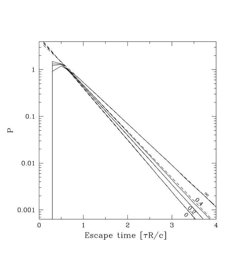
Figure 3: Distribution of low-frequency photons over the time of their escape from a cloud of electrons with an optical depth of $\tau=5$ ($R$ is the radius of the cloud), for various plasma temperatures (curves are labelled with the corresponding values of $kT_{e}/m_{e}c^{2}$). The solid lines are Monte-Carlo simulation results. The dashed lines show the results of the calculation by the approximate formula (16), which can be used for describing the exponential (power-law in the linear-logarithmic coordinates used) part of the distribution function. The diffusion coeffient $D$ appearing in equation (16) is given by Eq. (14) in the case $kT_{e}\gg m_{e}c^{2}$ and by Eq. (15) in the case $kT_{e}\mathrel{\hbox{\hbox to0.0pt{\hbox{\lower 4.0pt\hbox{$\sim$}}\hss}\hbox{$<$}}}0.4m_{e}c^{2}$.