The Local Space Density of Optically–Selected Clusters of Galaxies

Abstract

We present here new results on the space density of rich, optically–selected, clusters of galaxies at low redshift ($z<0.15$). These results are based on the application of the matched filter cluster–finding algorithm (as outlined by Postman et al. 1996 and Kawasaki et al. 1998) to $1067{\rm deg^{2}}$ of the Edinburgh/Durham Southern Galaxy Catalogue (EDSGC). This is the first major application of this methodology at low redshift and in total, we have detected $2109$ clusters above a richness cut–off of $R_{m}\geq 50$ (or $\Lambda_{cl}\geq 10$; Postman et al. 1996). This new catalogue of clusters is known as the Edinburgh/Durham Cluster Catalogue II (or EDCCII). We have used extensive Monte Carlo simulations to define the detection thresholds for our algorithm, to measure the effective area of the EDCCII and to determine our spurious detection rate. These simulations have shown that our detection efficiency is strongly correlated with the presence of large–scale structure in the EDSGC data. We believe this is due to the assumption of a flat, uniform background in the matched filter algorithm. Using these simulations, we are able to compute the space density of clusters in this new survey. We find $83.5^{+193.2}_{-36.9}\times 10^{-6}\,h^{-3}\,{\rm Mpc^{-3}}$ for $100\leq R_{m}<200$ ($\Lambda_{cl}\simeq 20$) systems, $10.1^{+11.3}_{-4.3}\times 10^{-6}\,h^{-3}\,{\rm Mpc^{-3}}$ for $200\leq R_{m}<400$ ($\Lambda_{cl}\simeq 40$) systems and $2.3^{+2.5}_{-2.3}\times 10^{-6}\,h^{-3}\,{\rm Mpc^{-3}}$ for $R_{m}>400$ ($\Lambda_{cl}>80$) systems. These three richness bands roughly correspond to Abell Richness Classes 0, 1 and $\geq 2$ respectfully. These new measurements of the local space density of clusters are in agreement with those found at higher redshift ($0.2<z_{est}<0.6$) in the Palomar Distant Cluster Survey (PDCS; Postman et al. 1996 & Holden et al. 1999) and therefore, removes one of the major uncertainties associated with the PDCS as it had previously detected a factor of $5\pm 2$ more clusters at high redshift than expected compared to the space density of low redshift Abell clusters. This discrepancy is now lessened and, at worst, is only a factor of $4^{+10}_{-4}$. This result illustrates the need to use the same cluster–finding algorithm at both high and low redshift to avoid such apparent discrepancies. We also confirm that the space density of clusters remains nearly constant out to $z\sim 0.6$ in agreement with previous optical and X–ray measurements of the space density of clusters (Couch et al. 1991; Postman et al. 1996; Ebeling et al. 1997; Nichol et al. 1999). Finally, we have compared the EDCCII with the Abell catalogue. We detect nearly 60% of all Abell clusters in the EDCCII area regardless of their Abell Richness and Distance Classes. For clusters in common between the two surveys, we find no strong correlation between the two richness estimates in agreement with the work of Lumsden et al. (1992). In comparison, $\sim 90\%$ of the EDCCII systems are new, although a majority of them have a richness lower than an Abell Richness Class of 0 and therefore, would be below Abell’s original selection criteria. However, we do detect 143 new clusters with $R_{m}\geq 100$ (which corresponds to a Richness Class of greater than, or equal to, 0) that are not in the Abell catalogue i.e. 63% of the rich EDCCII systems. These numbers lend credence to the idea that the Abell catalogue may be incomplete, especially at lower richnesses.

1. Introduction

Clusters of galaxies play a key role in tracing the distribution and evolution of mass in the universe (see, for example, Guzzo et al. 1992; Postman et al. 1992; Nichol et al. 1992, Dalton et al. 1992; Bahcall & Soneria 1983; Reichart et al. 1999). Until recently, such studies have been based on catalogues of clusters constructed from visual scans of photographic plates e.g. the Abell catalogue (Abell 1958; Gunn, Hoessel & Oke 1986; Abell et al. 1989; Couch et al. 1991). However, during the past decade, there has been considerable progress in the construction of automated catalogues of clusters and groups that possess objective selection criteria. Such work includes cluster catalogues selected from digitized photographic material (Dodd & MacGillivray 1986; Lumsden et al. 1992; Dalton et al. 1994), from X–ray surveys (Kowalski et al. 1984; Ebeling et al. 1997; de Grandi et al. 1999; Gioia et al. 1990; Nichol et al. 1997 & 1999; Rosati et al. 1998; Burke et al. 1997; Jones et al. 1998; Romer et al. 1999) and large–area optical CCD surveys (Postman et al. 1996; Lidman & Peterson 1996; Zaritsky et al. 1997; Olsen et al. 1999).

Figure 1.— The $10^{\circ}\times 10^{\circ}$ test region outlined in Section 2 and used for our simulations. Cluster detections within $5\times\theta_{c}$ (at $z=0.05$ this is $0.35^{\circ}$) of the edges of this data were discarded.

There has also been great progress in the development of new cluster–finding algorithms. The first automated cluster catalogues used simple variants on the “peak–finding” algorithm (Lumsden et al. 1992) or the percolation method (Dalton et al. 1994). In recent years, several new, more sophisticated, algorithms have become available including the matched filter algorithm – in several different flavors (Postman et al. 1996; Kawasaki et al. 1998; Kepner et al. 1999; Schuecker & Bohringer 1998) –, the wavelet–filter (Slezak et al. 1990), the “photometric redshift” method (Kodama et al. 1999), voronoi tessellations (Ramella et al. 1998) and the “density–morphology” relationship (Ostrander et al. 1998). The level of sophistication of these algorithms has increased in anticipation of high quality CCD survey data e.g. the Sloan Digital Sky Survey (SDSS; Gunn et al. 1998),

The early automated catalogues of optically–selected clusters have produced two important results. First, Postman et al. (1996) and Lumsden et al. (1992) both find evidence for a higher space density of clusters than that seen in the Abell Catalogue. For example, Postman et al. (1996) finds that the measured space density of clusters in the Palomar Distant Cluster Survey (PDCS) is a factor of $5\pm 2$ greater than that implied from the Abell catalogue. Second, the space density of PDCS clusters remains constant between $z=0.2$ and $z=0.6$, in agreement with the earlier work of Couch et al. (1991) and has been confirmed recently by Holden et al. (1999). If true, these results can be used to place strong constraints on the underlying galaxy evolution model (e.g. CDM) and measurements of the cosmological parameters $\sigma_{8}$ and $\Omega_{o}$ (see Bahcall, Fan & Cen 1997; Reichart et al. 1999; Holden et al. 1999).

To solidify these initial results, larger catalogues of clusters are required. Moreover, it is becoming increasingly clear that we need to compare these different cluster catalogues to help verify results and expand the redshift range over which we can study the cluster distribution. To date however, there has been little cross–comparison between these different cluster catalogues. Foremost, the relationship between the X–ray and optical catalogues of clusters remains unclear (see Holden et al. 1997; Briel & Henry 1993; Bower et al. 1997). In the optical domain, different catalogues have used different cluster finding algorithms thus making it very difficult to cross–calibrate catalogues and methods and thus verify results. This is illustrated by the fact that although both Lumsden et al. (1992) and Postman et al. (1996) find a higher space density than the Abell catalogue, the PDCS finds 5 times as many clusters per unit volume, while the Edinburgh–Durham Cluster Catalogue (EDCC; Lumdsen et al. 1992) only finds twice as many clusters per unit volume as Abell. Therefore, it is impossible to fairly compare the EDCC and the PDCS even though they are both objective, automated catalogues of clusters.

In this paper, we set out to rectify this problem by running a variant of the PDCS cluster–finding algorithm on the same galaxy data as used by Lumsden et al. (1992) in the construction of the EDCC. The main aim of this project is to provide a coherent set of cluster data that spans from $z\sim 0.05$ – the lower redshift limit of the EDSGC – to $z\simeq 0.6$ – the upper completeness limit of the PDCS. In addition to using a similar algorithm as Postman et al. (1996), we have performed a large number of Monte Carlo simulations to assess the completeness limit, and contamination rate, of this new EDCC cluster catalogue. This is the first major application of the matched filter algorithm to low redshift galaxy data, however, it is only the first of many such surveys presently underway e.g. the SDSS, DeepRange (Postman et al. 1998), DPOSS (Gal et al. 1999), COSMOS (Schuecker & Boehringer 1998) and the CCD survey of Zaritsky et al. (1997).

In Section 2, we discuss the EDSGC catalogue and the matched filter detection algorithm. In Section 3, we outline the methodology used to detect our cluster candidates and discuss in detail the Monte Carlo simulations we performed to determine our detection thresholds, the effective area of our new cluster survey and our spurious detection rate. Readers interested in just the results of this survey may wish to concentrate on Section 4 of this paper which presents our space density results. In Section 5, we discuss these results in comparison with the PDCS and Abell cluster catalogues. Throughout this letter, we use $H_{o}=100\,h\,{\rm kms^{-1}Mpc^{-1}}$ and $q_{o}=0.5$ unless otherwise stated.

	${\rm Redshift}\,\,(z_{est})$
$R_{m}$	0.05	0.07	0.09	0.12	0.15
50	270	210	190	220	320
100	310	270	230	250	320
200	410	340	340	350	410
400	600	480	460	480	540

Table 1Richness threshold values (RT) determined for various redshifts and cluster richnesses

2. The Edinburgh–Durham Southern Galaxy Catalogue

The Edinburgh–Durham Southern Galaxy Catalogue (EDSGC) has been discussed in detail in Heydon–Dumbleton et al. (1989), Lumsden et al. (1992), Collins et al. (1992), and Collins, Nichol, and Lumsden (2000). However, for consistency, we include here a brief discuss of the salient points of this catalogue.

The whole EDSGC comprises of  1.5 million galaxies brighter than $b_{j}=21.5$ covering an area of $\sim 1100$ squared degrees centered on the South Galactic Pole, spanning 90 degrees in Right Ascension and 20 degrees in declination. The catalogue is $95\%$ complete to $b_{j}=20$ and has $\leq 10\%$ stellar contamination. The catalogue was constructed from COSMOS (a microdensitometer) scans of UK Schimdt IIIa–J photographic survey plates and as photometrically calibrated using 30 CCD sequences positioned in a “checkerboard fashion”. From the EDSGC, Lumsden et al. (1992) detected $733$ galaxy overdensities using a simple “peak–finding” algorithm. Collins et al. (1995) presents 777 redshifts measurements within 94 clusters and this redshift sample has been used to study the large–scale distribution of nearby clusters (see Nichol et al. 1992, Guzzo et al. 1992 & Martin et al. 1995) as well as the cluster luminosity function (Lumsden et al. 1997).

	${\rm Redshift}\,\,(z_{est})$
$R_{m}$	0.05	0.07	0.09	0.12	0.15
50	-230	-130	-90	-65	-60
100	-230	-150	-90	-65	-65
200	-250	-160	-110	-80	-65
400	-360	-200	-140	-100	-70

Table 2Log likelihood threshold values (LT) determined for various redshifts and cluster richnesses

For the analysis discussion in Section 3, we restrict ourselves to a small $10^{\circ}\times 10^{\circ}$ random subregion of the EDSGC centered at $00^{hrs}$ $30^{mins}$ in Right Ascension and $-33^{\circ}$ in Declination. We also restricted the magnitude range to $15<b_{j}<20.5$ to remain as complete as possible (see Collins, Nichol & Lumsden 2000). These cuts resulted in a total of 41171 galaxies which is significantly smaller than the whole EDSGC. This test data is shown in Figure 1. For the space density results presented in Section 4, we used to all galaxies in the magnitude range $15<b_{j}<20.5$ and in a coordinate range of $22^{\rm hrs}<\alpha<3.3^{\rm hrs}$ and $-42^{\circ}<\delta<-23^{\circ}$ ($1067{\rm deg^{2}}$) which gave us 627260 galaxies in total.

We note here that the EDSGC has previously been used to construct an objective catalogue of clusters of galaxies (see Lumsden et al. 1992). However, in this prior analysis, only a simplistic “peak–finding” algorithm was used to find candidate systems for redshift follow–up. Given the recent advances in cluster–finding algorithms, we decided it was prudent to repeat the analysis which we discuss herein. We stress however that this does not undermine the scientific integrity of the original EDCC catalogue (Lumsden et al. 1992) and results derived from it (Nichol et al. 1992; Collins et al. 1995; Martin et al. 1995). In this present work, we simply wish to analyze the low redshift cluster population using the same techniques as presently used at high redshift (i.e. PDCS). For the sake of consistency, we call this new cluster catalogue the Edinburgh/Durham Cluster Catalogue II (EDCCII).

3. Methodology

3.1. The Matched Filter

In recent years, there has been considerable progress in the development of new, automated cluster–finding algorithms (see Lumsden et al. 1992; Dalton et al. 1994; Postman et al. 1996; Kawasaki et al. 1998; Kepner et al. 1999; Schuecker & Bohringer 1998; Slezak et al. 1990; Kodama et al. 1999; Ramella et al. 1998; Ostrander et al. 1998). In this paper, we focus our attention on the matched filter algorithm since we are interested in directly comparing our results to those of Postman et al. (1996).

We have based our matched filter algorithm on the procedure outlined by Kawasaki et al. (1998) which compares the galaxy distribution around any point on the sky to a cluster model plus a background (see Eqn. 1 in Kawasaki et al. 1998). The parameters of this cluster model are given in Eqns. 2, 3 & 4 of Kawasaki et al. (1998) and are the cluster surface density profile, the intrinsic richness of the cluster ($N$ in Eqn 1. of Kawasaki et al. 1998), the cluster and field luminosity functions and the surface density of background galaxies ($\sigma_{f}$). For the analysis discussed herein, we have modeled our clusters as a spherically–symmetrical, isothermal surface density profile (i.e. a King profile with $r_{core}=170$ kpc and $\beta=\frac{2}{3}$) combined with a Schechter luminosity function (with $M^{\ast}_{b_{j}}=-20.12$ and $\alpha=-1.25$; see Lumsden et al. 1997). The background galaxy distribution is modeled as a flat surface density of galaxies of $\sigma_{f}=583775$ galaxies per steradian which is the measured average surface density of galaxies in the EDSGC in the magnitude range $15<b_{j}<20.5$. For the field luminosity function ($\theta_{f}(m)$ in Eqn. 3 of Kawasaki et al. 1998), we used a Schtecter function with $M^{\ast}_{b_{j}}=-19.5$ and an $\alpha=-1.1$ (see Loveday et al. 1992).

The physical model for the cluster plus background is converted to an observational model using the standard cosmological redshift–distance relationships (and k–corrections) and therefore, the model is only a function of the intrinsic richness of the cluster and its redshift. This observed model is convolved with the data and a likelihood assigned for each point on the sky which is proportional to the quality of fit of the cluster model to the observed galaxy distribution given Possion statistics (see Eqns 6 & 7 of Kawasaki et al. 1998). One can then maximized the likelihood by varying the two parameters of the model i.e. richness and redshift. Computationally, this was achieved by overlaying the EDSGC with a grid (pixel scale of $\theta_{c}/3$), and comparing each pixel, in this grid, with the matched filter model as a function of cluster redshift and richness ($R_{m}$). For the results presented herein, we varied the matched filter redshift ($z_{est}$) from $0.05$ to $0.15$ ($\delta z_{est}=0.0025$) and used richness estimates of $R_{m}=50$, 100, 200 and 400. This resulted in an array of likelihood and richness maps (see Kawasaki et al. 1998) from which we must select our cluster candidates.

3.2. Monte Carlo Simulations

In this section, we outline our Monte Carlo simulations which were used to determine the cluster detection thresholds as well as to estimate our spurious cluster detection rate and overall cluster detection efficiency.

3.2.1 Model of a Cluster

For our Monte Carlo simulations, we must first create an artificial cluster. We used a spherically–symmetrical, isothermal surface density profile with a cluster core radius ($r_{c}$) of $170$ kpc, a cutoff radius of $5r_{c}$ and a Schtecter luminosity function with $\alpha=-1.25$ and $M^{\ast}_{B}=-20.12$ (we restricted ourselves to an absolute magnitude range of $M^{\ast}_{b_{j}}\pm 5$). This artificial cluster was then redshifted appropriately using the standard cosmological relations and

$$m=M+(42.384+5\log z)+(4.14z-0.44z^{2}),$$ (1)

to convert absolute magnitude to apparent $b_{j}$ magnitude (see Lumsden et al. 1997). To match the magnitude range covered by the EDSGC survey, we then removed all galaxies outside the magnitude range of $15<b_{j}<20.5$. Four different intrinsic richnesses of artificial cluster were used in our Monte Carlo simulations; $R_{m}=50,\,100,\,200,\,\&\,400$. Unless otherwise stated, each artificial cluster was unique, with the galaxies distributed at random according to the angular and luminosity distributions given above.

We note here that no attempt was made to simulate the density–morphology relationship or to allocate a cD–type galaxy at the cluster core. Moreover, we did not change the shape or parameters of our artificial clusters during our simulations. Such simulations would have been computational intensive but are clearly needed in the future.

more would have resulted in merging of the artificial clusters, while adding fewer clusters would have made the simulations laborious. We then varied the thresholds, both in richness (RT) and likelihood (LT), and computed for each combination the number of artificial clusters detected as well as the total number of clusters detected above these thresholds.

It was then necessary to weight these detections to determine the optimal thresholds. Clearly, we wish to rule out obvious cases i.e. detecting 1 artificial cluster while detecting hundreds of other systems within the EDSGC (as most of these detections will be either lower richness clusters or spurious detections). Unfortunately, most cases we encountered were more subtle than this i.e. detecting 10 artificial clusters within a total of 25 detections, or detecting 15 artificial clusters within a total 40 detections. To help differentiate between these intermediate cases, we employed an analytical method which we outline below.

We defined the number of detections of our artificial clusters to be $x$ and the number of total detections to be $y$. Both $x$ and $y$ are functions of RT and LT and increase with decreasing thresholds. We therefore defined a function (T($x,y$)) which satisfied the following boundary conditions; T($0,y$)$=0$, $\lim_{y\rightarrow\infty}$ T($x,y$) $=0$ and the maximum of T($x,y$) is at T($20,20$). The functional form of T($x,y$) is therefore important since it is now our weighting scheme. We estimated T($x,y$) by running our cluster–finding algorithm over many thousands of realizations of our simulations and varying RT and LT to create a Monte Carlo estimate for T$(x,y)$. From these data, we empirically found that T($x,y$)$=\frac{x^{3}}{y^{1.3}}$ was the best functional form for this data and adopted it as our weighting scheme. Using this relationship, we then determined the optimal RT and LT thresholds as a function of redshift and intrinsic richness. Our thresholds are given in Tables 1 and 2 (we used linear interpolation between these values if necessary).

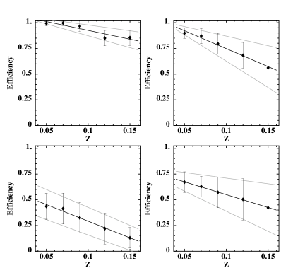
Figure 2.— The averaged measured detection efficiency for clusters of various richness as a function of redshift. Clockwise from the upper left–hand panel, the graphs represent clusters of richnesses $R_{m}=$ 400, 200, 100, and 50.

3.2.2 Locating Cluster Candidates

In this subsection, we review our procedure for identifying a unique cluster candidate above the thresholds outlined above. We first designate all pixels in our likelihood and richness maps that satisfy our thresholds, $\geq$RT and $\geq$LT, as “active” pixels. Obviously, a single cluster candidate will create multiple active pixels so we must group these pixels together into single detection. This is achieved by searching for peaks in the distribution of active pixels i.e. we look for a active pixel whose height is greater than any other active pixel within a radius of $2{\theta_{c}}$ of the peak. We then group together all active points in this area to create a unique cluster candidate. If a single active pixel is a peak by default – i.e. there are no other active pixels within $2\theta_{c}$ of it – we disregard this peak and do not include it in our final analysis. Such isolated peaks are unlikely to be caused by real clusters. Finally, we compute the weighted mean of all active points grouped together as a single cluster to determine the most likely cluster candidate centroid.

3.2.3 Determining Detection Efficiencies

In addition to determining our detection thresholds, our Monte Carlo simulations were used to estimate our detection efficiency and the effective area of our cluster search. This is an important aspect of any cosmological survey as it allows us to determine the volume sampled by the EDCCII and thus measure the space density of clusters from the catalogue. Previous applications of automated optical cluster–finding algorithms have based their efficiency measurements on their ability to detect clusters within artificial galaxy data. For example, Postman et al. (1999) and Kepner et al. (1999) created artificial galaxy catalogues with the same statistical properties as real galaxy catalogues e.g. they matched the surface density of galaxies and/or the large–scale clustering properties of the galaxies. They then added artificial clusters to such simulated galaxy data.

We however found this method inadequate since such simulated galaxy catalogues cannot fully reproduce the hierarchical structure of galaxies in the universe. Specifically, the effects of superpositions of structures, variations in the field counts, or large–scale structures are hard to include in these simulations. Therefore, for each combination of RT and LT (see Tables 1 and 2), we added a total 6000 artificial clusters (20 at a time) at random in the EDSGC and computed our success rate in detecting these artificial clusters above our thresholds (an artificial cluster was considered detected if a candidate cluster was found by our algorithm within $2\theta_{c}$ of the original coordinate of the artificial cluster; $\theta_{c}$ was evaluated at the redshift of the artificial cluster).

In Figure 2, we present our average detection efficiencies as a function of input redshift and richness (using the $10^{\circ}\times 10^{\circ}$ test area discussed in Section 2 and in Figure 1). The error bars are the standard deviation observed between the different trials of 20 clusters added to the EDSGC data at any one time.

In Figure 3, we show an example of the angular dependence of our detection efficiency. It is interesting to note that our efficiency is strongly correlated with the large–scale structure (LSS) in the Universe. This effect is most prominent for lower richness clusters, while for the richer systems ($R_{m}\geq 200$), it is insignificant (except at the highest redshifts probed by our simulations where the effect resulted in a loss of $\simeq 15\%$ of artificial clusters). In addition to this interference, our efficiency in detecting low richness, high redshift clusters was hindered by the magnitude limit of the EDSGC data since the number of potentially visible galaxies in these artificial clusters decreases below the noise in the background.

This problem of LSS interference appears to effect both over– and under–dense regions of the EDSGC data (when compared to the mean surface density of galaxies). For example, the most striking example of this LSS interference is seen at coordinates 2.0, 7.5 in Figure 1, where a group of clusters – Abell 2730, 2721, 2749, 2755, and 12S – has reduce our detection efficiency to almost zero (see Figure 3 ). In contrast, we also observe in Figure 3 a low detection efficiency near coordinates 8.0, 6.0 which coincides with a under–dense region in Figure 1. We believe this effect is caused by our assumption of a flat, uniform galaxy background as used in the matched filter algorithm (see Section 3.1). In both over– and under–dense regions, our assumption of a flat background with the mean surface density of the EDSGC is poor and therefore, we suppress the overall likelihood of the cluster detection i.e. the model of the background around the cluster is not a flat surface density of $\sigma_{f}=583775$ galaxies per steradian. This effect is further exasperated by systematic plate–to–plate uncertainties in the magnitude zero-point of the EDSGC photographic plates (Nichol & Collins 1993).

	${\rm Redshift}\,\,(z_{est})$    (${\rm deg^{2}}$)
$R_{m}$	0.05	0.07	0.09	0.12	0.15
50	580	516	415	266	196
100	742	687	612	553	445
200	962	928	855	729	594
400	1067	1063	1034	966	908

Table 3The effective area (${\rm deg^{2}}$) of the EDCCII as a function of input cluster redshift and richness. These numbers were extrapolated from the efficiencies we derived for the smaller test area of the EDSGC.

We present the effective area of the whole EDCCII in Table 3 based on our simulation results. These data were obtained by summing over the larger EDSGC survey area, as defined in Section 2, but weighted by our success rate in detecting artificial clusters as computed from the smaller test area. The data given in Table 3 illustrate the power of this new EDCCII catalogue since we now know the selection function of an optically–selected cluster catalogue to the same accuracy as a X–ray–selected cluster survey (e.g. Nichol et al. 1999). This effective area will be used below when calculating the space density of clusters (see Section 4)

3.2.4 Determining Spurious Detection Rate

The final use of our simulations was to determine the likely spurious detection rate. Again, we have tried to use the real galaxy data as much as possible in this analysis so as to mimic the real uncertainties in the EDSGC catalogue. This is different from previous attempts to estimate the spurious detection rate which have relied on simulated galaxy catalogues (see Postman et al. 1996).

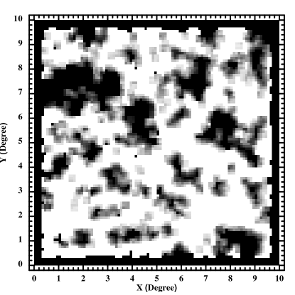
Figure 3.— Our detection efficiency as a function of position in the EDSGC data shown in Figure 1. Light areas indicate a detection efficiency of $100\%$ for our artificial clusters, while dark areas indicate a 0% detection efficiency. Efficiencies near the edge of the area were not measured. This plot is for $z_{est}=0.05$ and $R_{m}=100$ artificial clusters.

To achieve this goal therefore, we perturbed each galaxy in the EDSGC in a random distance (between $2\theta_{c}$ and $5\theta_{c}$ with a flat distribution) in a random direction from its original position. This procedure effectively smoothes the galaxy catalogue on these particular scales removing all small–scale structure in the catalogue while retaining the large–scale features within the catalogue. We then applied our matched filter algorithm to these perturbed galaxy catalogues and calculated the number of clusters that would satisfy our selection criteria. This was performed many thousands of times to determine the standard deviation in our spurious detection rate.

Figure 4.— Number of spurious detections as a function of redshift for $R_{m}=50$ (top) and $R_{m}=100$ (bottom) clusters in our 10x10 EDSGC test area. Number of spurious detections for higher richness clusters were negligible i.e. less than one spurious cluster in the $10^{\circ}$x$10^{\circ}$ area.

Our spurious detection rates are shown in Figure 4. The number of spurious detections was significant only for high redshift $R_{m}=50$ and $R_{m}=100$ clusters. Based on these simulations therefore, we restrict ourselves to $z\leq 0.12$ for $R_{m}\leq 100$ and $z\leq 0.15$ for $R_{m}>100$ to ensure that the spurious detection rate remains insignificant. For example, for $R_{m}\geq 200$ systems, $<1\%$ of detected clusters are likely to be spurious below $z=0.15$. We also exclude all clusters at $z<0.05$ as our thresholds are not accurately calibrated below this redshift. In Section 4 therefore, we restrict ourselves to $R_{m}\geq 100$ systems in the redshift range $0.05<z<0.15$ and make no correction for spurious detections within this richness and redshift range.

We note here that the results of these simulations are in good agreement with empirical determinations of the completeness of the EDSGC and EDCC catalogues i.e. based on 777 galaxy redshift measurements, Nichol (1993) showed that the EDCC was complete out to $z\simeq 0.13$ and only contained $<15\%$ contamination from spurious clusters. At low redshift, Lumsden et al. (1992) also had difficulty detecting $z<0.03$ clusters in the original EDCCI catalogue because of the large angular size subtended by such clusters.

In addition to randomizing the positions of the EDSGC, we also performed simulations which randomly shuffled the magnitudes of the galaxies throughout the EDSGC data. This resulted in galaxy catalogues with the same statistical properties – i.e. same angular clustering and number–magnitude relationship – but removed all correlations with magnitude. Again, these randomized catalogues were analyzed with our matched filter algorithm and resulted in a very similar result as presented in Figure 4 i.e. the spurious detection rate was insignificant for lower redshift, higher richness systems. We note however, that on average we detected fewer rich systems than with the real EDSGC data. In other words, magnitude correlations only appear to aid in the detection of rich clusters in the data.

3.2.5 Merging of Catalogues

Once we have the cluster detections, as a function of redshift and richness, we must then remove duplicate cluster detections to produce a final catalogue of unique cluster candidates. This was achieved by grouping together all systems whose measured centroids were within $2\,\times\,\theta_{c}$ of each other. We began this process by grouping together candidates as a function of their redshift, followed by their richness. If duplicates were found, we simply averaged their richness and redshift estimates to obtain a final estimate of the candidate clusters’ richness and redshift.

4. The Space Density of EDCCII Clusters

	$N(\geq R_{m}(\Lambda_{cl}),\leq z_{est})\,\,\,({\rm deg^{2}})$
$R_{m}$ ($\Lambda_{cl}$)	$0.12$ or $0.15$	$0.3$	$0.4$	$0.6$
$R_{m}\geq 100$ ($>20.3$)	$0.41^{+0.72}_{-0.23}$ ($z_{est}\leq 0.12$)	$3.1$	$4.9$	$7.6$
$R_{m}\geq 200$ ($>40.6$)	$0.074^{+0.075}_{-0.029}$($z_{est}\leq 0.15$)	$1.4$	$3.2$	$5.9$
$R_{m}\geq 400$ ($>81.2$)	$0.015\pm 0.015$ ($z_{est}\leq 0.15$)	$0.015$	$0.4$	$1.4$

Table 4Comparison of cumulative surface densities of the EDCCII and the PDCS. The cumulative surface densities of the PDCS clusters were calculated using the data in Table 4 of Postman et al. (1996) using the EDCCII as a zero point. We excluded all PDCS clusters with $\sigma<3$ and a radius of $>200$ since such clusters have a higher probability of being spurious (see Postman et al. 1996). We assumed $5.1\,{\rm deg^{2}}$ for the surface area of the PDCS survey. Our PDCS surface densities agree with those presented in Figure 21 of Postman et al. (1996). The EDCCII data presented in this table has not been corrected for spurious detections.

In the section, we present the results of applying the match filter algorithm as outlined in Section 3 to the whole EDSGC (as defined in Section 2). However, we must first establish a common framework within which to compare our results with previous studies. To this end, we will quote our results both as a function of $\Lambda_{cl}$, the cluster richness as defined by Postman et al. (1996) for the PDCS catalogue, and $R_{m}$, which is defined by us. As $R_{m}$ and $\Lambda_{cl}$ are just different richness normalizations of the match filter model (see Section 3.1), it is easy to relate the two analytically. This was achieved by integrating a normalized Schtecter function of richness $R_{m}$ over the luminosity range discussed in Section 3.1 and dividing by $L^{\star}$, the characteristic luminosity of the Schtecter function. This is equivalent to the original definition of $\Lambda_{cl}$ in Postman et al. (1996). Using $\alpha=-1.1$ (Postman et al. 1996), we show that $\Lambda_{cl}=20.3$ is $R_{m}=100$, $\Lambda_{cl}=40.6$ is $R_{m}=200$ and $\Lambda_{cl}=81.2$ is $R_{m}=400$. We quote here $\Lambda_{cl}$ in the PDCS $V_{4}$ passband as this is closest to the EDSGC $b_{j}$ passband.

In addition to comparing with the PDCS, we wish to compare with the original Abell catalogue. We achieve this by combining the equality $N_{R}(1.0)/N_{R}(1.5)\simeq 0.7$ (taken from Postman et al. 1996) with Figure 17 of Postman et al. (1996) to obtain an empirical relationship of $R_{abell}\sim 2\times\Lambda_{cl}$ for low redshift clusters ($z\leq 0.2$). Therefore, the three $\Lambda_{cl}$ richnesses given above approximately correspond to Abell Richness Classes (RC) 0, 1 and 2 respectively. These conversions are in good agreement with those presented in Lubin & Postman (1996 and references therein) and used by others (Holden, private communications; Postman, private communications). For the rest of this paper, we concentrate on the $R_{m}\geq 100$ systems ($\Lambda_{cl}\geq 20$ or ${\rm RC}\geq 0$).

In Table 4, we present the cumulative surface densities of EDCCII clusters using the methodology outlined in this paper. To compute these surface densities, as a function of richness, we have summed the number of unique clusters with richnesses of $\geq R_{m}$, divided by the effective areas in Table 3. The upper error bars quoted in Table 4 were computed by assuming all clusters detected at a particular richness are valid cluster candidates i.e. if we count all clusters at that richness regardless of duplicate entries (see Section 2). The lower error bars were computed using clusters only detected at that richness i.e. they were not detected at any other $R_{m}$ value. We note that these error bars are conservative and should be viewed as boundary values.

In Table 5, we present the EDCCII space densities along with cluster space density measurements from the PDCS, Holden et al. (1999) and the Abell catalogue. For the EDCCII, we computed the space densities of clusters, as a function of richness($n(R_{m})$) using the formula

$$n(R_{m})=\sum^{Z_{slices}}\frac{N(z_{est},R_{m})}{\int_{z_{2}}^{z_{1}}\,V(z)\times\Omega(R_{m},z_{est})},$$ (2)

which is a sum over all appropriate redshift slices ($Z_{slice}$). Here, $V(z)$ is the differential cosmological volume (per ${\rm deg^{2}}$), $\Omega(R_{m},z_{est})$ is the effective area as a function of redshift in Table 3, $N(z_{est},R_{m})$ is the number of clusters detected within a redshift slice for a given richness $R_{m}$, $z_{1}$ and $z_{2}$ are the limits of integration for the redshift slice. For $R_{m}\leq 100$, we have summed out to $z_{est}=0.12$, while for $R_{m}>100$, we sum to $z_{est}=0.15$. The error bars on these measurements were estimated using the same methodology as discussed above for the EDCCII cluster surface densities.

5. Discussion

Recently, Holden et al. (1999) published $84$ redshift measurements towards $16$ low redshift PDCS clusters. From these data, Holden et al. (1999) showed that the matched filter redshift estimate for $z_{est}<0.5$ PDCS clusters had an error of only $\delta z\simeq 0.07$; much smaller than previously quoted by Postman et al. (1999). Therefore, in Table 5, we present our estimates of the PDCS space density of low redshift clusters ($0.2<z_{est}<0.6$) using the PDCS $z_{est}$ measurements and the data given in Table 4 of Postman et al. (1996). We have excluded all PDCS clusters with $\sigma<3$ and a radius of $>200$, in the ${\rm V_{4}}$ data, to minimize the effects of spurious detections (see Postman et al. 1996). Therefore, these space densities may be lower than expected since we have potentially excluded some real clusters as well. This approach is valid as the true error on $z_{est}$ is now significantly smaller than our redshift slice i.e. a substantial number of clusters will not be scattered in, or out, of our sample because of the error in $z_{est}$.

	Cluster Space Densities ($10^{-6}\,h^{-3}{\rm Mpc^{-3}}$)
$n(R_{m})$	EDCCII	PDCS	Holden et al.	Abell
$100\leq R_{m}<200$ ($\simeq 20\leq\Lambda_{cl}<40$; RC$\sim$0)	$83.5^{+193.2}_{-36.9}$	$6.9^{+6.1}_{-3.6}$		$11.3$
$200\leq R_{m}<400$ ($\simeq 40\leq\Lambda_{cl}<80$; RC$\sim$1)	$10.1^{+11.3}_{-4.3}$	$12.8^{+7.6}_{-5.0}$	$31.3^{+30.5}_{-17.1}$	$4.04$
$R_{m}\geq 400$ ($\simeq\Lambda_{cl}>80$; ${\rm RC}\geq 2$)	$2.3^{+2.5}_{-2.3}$	$9.4^{+6.8}_{-4.7}$	$10.4^{+23.4}_{-8.4}$	$1.58$

Table 5Comparison of space density measurements of the EDCCII, PDCS and Abell catalogues. The EDCCII space densities were calculated using Equation 1. The error bars for the EDCCII catalogue are discussed in the text, while we quote 68% error bars for the Holden et al. space densities as taken from their paper.

For the $40\leq\Lambda_{cl}<80$ (RC$\sim$1) clusters, we find good agreement between the PDCS and EDCCII space densities. The same can not be said for the RC$\sim$0 systems where we differ by over an order of magnitude. We believe this discrepancy is the combination of two effects. First, the PDCS contains very few $\Lambda_{cl}<30$ clusters indicating that the catalogue is possibly incomplete at these low richnesses (the PDCS only contains 7 such systems at these low richnesses). Secondly, the EDCCII may slightly overestimate the space density of low richness clusters as the matched filter tends to de–blend rich, nearby systems ($z<0.05$) into several lower richness clusters. Therefore, we will not discuss this inconsistency any further but note that this measurement will be important for the next generation of large–area CCD cluster surveys since they will possess the volume to probe the lower richness systems at high redshift. The EDCCII data will provide an important zero–point for such surveys (DeepRange, Zaritsky et al. 1997). For ${\rm RC}\geq 2$ systems, the EDCCII appears to find a factor of $\sim 4$ fewer clusters than the PDCS, however, the significance of this discrepancy is small given the (Poisson) errors on all measurements.

In addition to checking the matched filter redshift estimates, Holden et al. (1999) also computed the space density of PDCS clusters using a new, and completely independent, survey selection function than that used by Postman et al. (1996) and in this paper. Their results are presented in Table 5 and, within the errors, are in good agreement with both our PDCS and EDCCII space density measurements. Moreover, Holden et al. (private communication) have recently re-calculated their measurements of the PDCS space density, as given in Holden et al. (1999) and Table 5, but now based on a much larger sample of galaxy redshifts (over 700 redshifts in total). They now find $\sim 18\times 10^{-6}\,h^{-3}\,{\rm Mpc^{-3}}$ for RC=1 systems and $\sim 7\times 10^{-6}\,h^{-3}\,{\rm Mpc^{-3}}$ for ${\rm RC}\geq 2$ systems which is closer to the EDCCII space densities presented in this paper.

In summary, we find good agreement between all three of these surveys (PDCS, Holden et al. and the EDCCII) which combined span a redshift range of $0.05\leq z\leq 0.6$. At worst, the difference between the three surveys is $4^{+10}_{-4}$ (Table 3). This therefore justifies our original desire to run the matched filter algorithm on the low redshift EDSGC data since we are now comparing clusters selected in a similar way over this entire redshift range. We have thus removed one of the main uncertainties associated with the PDCS as we do not see a significant difference between the low and high redshift cluster populations (as originally highlighted by Postman et al. 1996). Moreover, this agreement implies that there is little evolution in the space density of optical clusters out to $z\simeq 0.5$, in agreement with results from X–ray surveys of clusters (see Nichol et al. 1997, 1999; Burke et al. 1997; Rosati et al. 1998; Vikhlinin et al. 1998; Ebeling et al. 1997, 1999). However, we should not overstate this claim, since the error bars on all measurements are large. In the future, we will need large samples of clusters that span a large range in redshift; this should be possible with the next generation of cluster catalogues constructed from surveys like DPOSS (Gal et al. 1999) and the SDSS (Gunn et al. 1998). We also urge the community to adopt one cluster–finding algorithm so it can be applied to different catalogues (at high and low redshift) consistently.

In Table 5, we present the space density of Abell clusters taken from Postman et al. (1996 and references therein). The EDCCII space density measurements appear to be systematically higher than the Abell catalogue e.g. we find $\sim 7$ times as many RC$\sim$0 clusters as Abell. However, for ${\rm RC>0}$, this discrepancy is much less while the errors on these measurements are large. Therefore, we must be wary about over–interpretating any claimed discrepancy with Abell and simply note that overall, the EDCCII has lessened the discrepancy previously claimed to be between the high and low redshift cluster populations.

Our potential disagreement with the Abell catalogue could be due to two factors. First, like the EDCCII catalogue, the effective area of the Abell catalogue could be smaller than expected (see Section 3). Secondly, the EDCCII could be finding more clusters than the Abell catalogue at a given richness. The first of these two factors is hard to quantify given the subjective nature of the Abell catalogue, however, the second factor can be addressed by cross–correlating individual clusters in both the EDCCII and Abell catalogues. We discuss the latter below.

In total, we detect 182 of the 324 Abell clusters in the EDCCII area, or 56% of them (using a matching radius of $7.5$ arcmins). This is in good agreement with Lumsden et al. (1992) who find $\sim 70\%$ match–up between their original EDCC clusters and the Abell catalogue. In both cases, the percentage of match–ups is independent of richness i.e. neither the EDCC or EDCCII appear to have missed Abell clusters of a particular richness class (see Figure 8 of Lumsden et al.). In addition to comparing richnesses, we have also compared the distance estimates of our matched, and unmatched, Abell clusters and find little correlation. Therefore, the missing $\sim 40\%$ of Abell clusters in the EDCCII catalogue appear to be spread evenly over all Richness and Distance Classes. Finally, for clusters in common between the EDCCII and Abell catalogues, we find no correlation between the two difference richness estimates i.e. $R_{m}$ and Abell richness or RC. This agrees with Lumsden et al. (1992) and Postman et al. (1996) both of whom detect a large scatter between their richness estimates and the Abell richness estimates.

In contrast, there are a total of 2109 EDCCII clusters detected in the area given in Section 2; a factor of $\sim 8$ more than detected in the Abell catalogue over the same area (we have excluded the supplementary Abell catalogue here and in the above analysis). This discrepancy is lessened when we consider only $R_{m}\geq 100$ systems where we find 227 EDCCII clusters (however, we note that the EDCCII only probes to $z_{est}\leq 0.15$, while the Abell catalogue contains rich systems out to $z\sim 0.4$). These raw numbers reflect the differences in the space densities measurements outlined in Table 5 and highlight that a vast majority of the new EDCCII systems are of lower richness (in the EDCCII catalogue). Although, we do note that $143$ of the $227$ $R_{m}\geq 100$ systems (63%) are not in the Abell catalogue (which corresponds to ${\rm RC\geq 0}$ systems). Again, these findings agree with the original EDCC cluster catalogue where almost 70% of EDCC clusters were new compared to the Abell catalogue. These two surveys therefore lend credence to the idea (already stated by Abell 1958 and Abell et al. 1989) that the Abell catalogue should not be used for statistical studies.

6. Acknowledgements

The authors would like to thank Brad Holden, Lori Lubin, Marc Postman and Kath Romer for their assistance during the course of this work. We also thank Chris Collins, Stuart Lumsden, Luigi Guzzo and Harvey MacGillivray for allowing us free access to the EDSGC data. This project was funded through NASA grant NAG5-3202 (RCN) and two CMU Summer Undergraduate Research Grants (DAB).

7. References

Abell, G. O., 1958, ApJS, 3, 211
Abell, G. O., Corwin, H. G. Jr., Olowin, R. P., 1989, ApJS, 70, 1
Bahcall, N. A., Soneira, R. M., 1983, ApJ, 270, 20
Bahcall, N. A., Fan, X., Cen, R., 1997, ApJ, 485L, 53
Bower, R. G., Castander, F. J., Ellis, R. S., Couch, W. J., Boehringer, H., 1997, MNRAS, 291, 353
Briel, U. G., Henry, J. P., 1993, A&A, 271, 413
Burke, D. J., Collins, C. A., Sharples, R. M., Romer, A. K., Holden, B. P., Nichol, R. C., 1997, ApJ, 488L, 83
Collins, C. A., Nichol, R. C., Lumsden, S. L., 1992, MNRAS, 254, 295
Collins, C. A., Guzzo, L., Nichol, R. C., Lumsden, S. L., 1995, MNRAS, 274, 1071
Collins, C. A., Nichol, R. C., Lumsden, S. L., 2000, ApJS, in preparation
Couch, W. J., Ellis, R. S., Maclaren, I., Malin, D. F., 1991, MNRAS, 249, 606
Dalton, G. B., Efstathiou, G., Maddox, S. J., Sutherland, W. J., 1992, ApJ, 390L, 1
Dalton, G. B., Efstathiou, G., Maddox, S. J., Sutherland, W. J., 1994, MNRAS, 269, 151
de Grandi, S., Boehringer, H., Guzzo, L., Molendi, S., Chincarini, G., Collins, C., Cruddace, R., Neumann, D., Schindler, S., Schuecker, P., Voges, W., 1999, ApJ, 514, 148
Dodd, R. J., Macgillivray, H. T., 1986, AJ, 92, 706
Ebeling, H., Edge, A. C., Fabian, A. C., Allen, S. W., Crawford, C. S., Boehringer, H., 1997, ApJ, 479L, 101
Ebeling, H., Jones, L.R., Perlman, E., Scharf, C., Horner, D., Wegner, G., Malkan, G., Fairley, B., Mullis, C.R., ApJ, submitted (astro-ph/9905321)
Gal, R. R., DeCarvalho, R. R., Odewahn, S. C., Djorgovski, S. G., Margoniner, V. E., 1999, AJ, astro-ph/9906480
Gioia, I. M., Henry, J. P., Maccacaro, T., Morris, S. L., Stocke, J. T., Wolter, A., 1990, ApJ, 356L, 35
Gunn, J. E., Hoessel, J. G., Oke, J. B., 1986, ApJ, 306, 30
Gunn, J. E., et al., 1998, AJ, 116, 3040
Guzzo, L., Collins, C. A., Nichol, R. C., Lumsden, S. L., 1992, ApJ, 393L, 5
Heydon-Dumbleton, N. H., Collins, C. A., Macgillivray, H. T., 1989, MNRAS, 238, 379
Holden, B. P., Romer, A. K., Nichol, R. C., Ulmer, M. P., 1997, AJ, 114, 1701
Holden, B. P., Nichol, R. C., Romer, A. K., Metevier, A., Postman, M., Ulmer, M. P., Lubin, L. M., 1999, AJ, astro-ph/9907429
Jones, L. R., Scharf, C., Ebeling, H., Perlman, E., Wegner, G., Malkan, M., Horner, D., 1998, ApJ, 495, 100
Kawasaki, W., Shimasaku, K., Doi, M., Okamura, S., 1998, A&AS, 130, 567
Kepner, J., Fan, X., Bahcall, N., Gunn, J., Lupton, R., Xu, G., 1999, ApJ, 517, 78
Kodama, T., Bell, E. F., Bower, R. G., 1999, MNRAS, 302, 152
Kowalski, M. P., Cruddace, R. G., Wood, K. S., Ulmer, M. P., 1984, ApJS, 56, 403
Lidman, C. E., Peterson, B. A., 1996, AJ, 112, 2454
Loveday, J., Peterson, B. A., Efstathiou, G., Maddox, S. J., 1992, ApJ, 390, 338
Lubin, L. M., Postman, M., 1996, AJ, 111, 1795
Lumsden, S. L., Nichol, R. C., Collins, C. A., Guzzo, L., 1992, MNRAS, 258, 1
Lumsden, S. L., Collins, C. A., Nichol, R. C., Eke, V. R., Guzzo, L., 1997, MNRAS, 290, 119
Martin, D. R., Nichol, R. C., Collins, C. A., Lumsden, S. A., Guzzo, L., 1995, MNRAS, 274, 623
Nichol, R. C., Collins, C. A., Guzzo, L., Lumsden, S. L., 1992, MNRAS.255, 21P
Nichol, R. C., 1993, PhD. Thesis, Univ. of Edinburgh
Nichol, R. C., Collins, C. A., 1993, MNRAS, 265, 867
Nichol, R. C., Holden, B. P., Romer, A. K., Ulmer, M. P., Burke, D. J., Collins, C. A., 1997, ApJ, 481, 644.
Nichol, R. C., Romer, A. K., Holden, B. P., Ulmer, M. P., Pildis, R. A., Adami, C., Merrelli, A. J., Burke, D. J., Collins, C. A., 1999, ApJ, 521, 21
Olsen, L. F., Scodeggio, M., Da Costa, L., Benoist, C., Bertin, E., Deul, E., Erben, T., Guarnieri, M. D., Hook, R., Nonino, M., Proni, I., Slijkhuis, R., Wicenec, A., Wichmann, R., 1999, A&A, 345, 681
Ostrander, E. J., Nichol, R. C., Ratnatunga, K. U., Griffiths, R. E., 1998, AJ, 116, 2644
Postman, M., Huchra, J. P., Geller, M. J., 1992, ApJ, 384, 404
Postman, M., Lubin, L. M., Gunn, J. E., Oke, J. B., Hoessel, J. G., Schneider, D. P., Christensen, J. A., 1996, AJ, 111, 615 (PDCS)
Postman, M., Lauer, T. R., Szapudi, I., Oegerle, W., 1998, ApJ, 506, 33
M. Ramella, M., Nonino, M., Boschin, W., Fadda, D., 1998, astro-ph/9810124
Reichart, D. E., Nichol, R. C., Castander, F. J., Burke, D. J., Romer, A. K., Holden, B. P., Collins, C. A., Ulmer, M. P., 1999, ApJ, 518, 521
Romer, A. K., Nichol, R. C., Holden, B. P., Ulmer, M. P., Pildis, R. A., Adami, C., Merrelli, A. J., Kron, R., Burke, D. J., Collins, C. A., 1999, ApJS, accepted
Rosati, P., Della Ceca, R., Norman, C., Giacconi, R., 1998, ApJ, 492L, 21
Schuecker, P., Boehringer, H., 1998,A&A, 339, 315
Slezak, E., Bijaoui, A., Mars, G., 1990, A&A, 227, 301
Vikhlinin, A., McNamara, B. R., Forman, W., Jones, C., Quintana, H., Hornstrup, A., 1998, ApJ, 502, 558
Zaritsky, D., Nelson, A. E., Dalcanton, J. J., Gonzalez, A. H., 1997, ApJ, 480L, 91