Abstract

We show that, in the context of Moore’s Law, overall productivity can be increased for large enough computations by ‘slacking’ or waiting for some period of time before purchasing a computer and beginning the calculation.

According to Moore’s Law, the computational power available at a particular price doubles every 18 months. Therefore it is conceivable that for sufficiently large numerical calculations and fixed budgets, computing power will improve quickly enough that the calculation will finish faster if we wait until the available computing power is sufficiently better and start the calculation then.

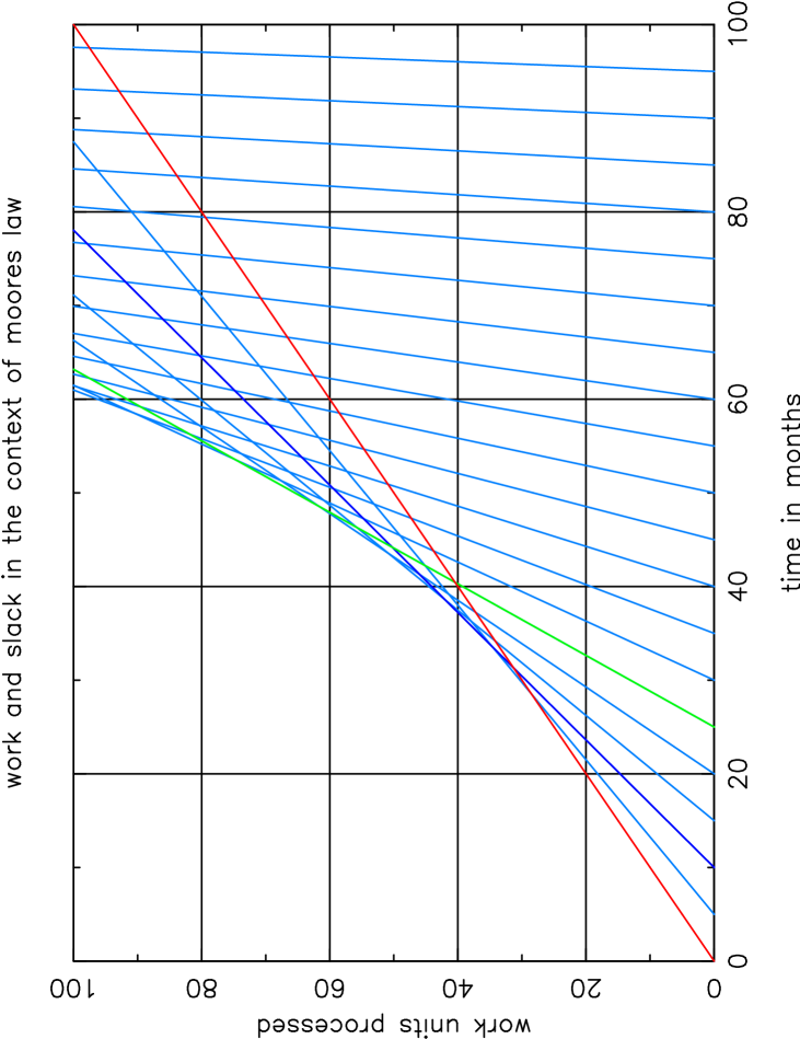
Figure 1:

This is illustrated in the above plot. Work is measured in units of whatever a current machine can accomplish in one month and time is measured in months. The red line denotes the amount of work completed if you start calculating now. However, according to Moore’s law the speed of computation, $R$, grows as $R_{t}=R_{0}2^{t/18mo}$. In our units $R_{0}=1$. If you wait some amount of time, then buy a new computer and begin the computation, Moore’s law ensures that the new computer will be faster, and you will get a steeper performance curve. The blue lines illustrate the performance you will get if you wait five, ten, or more months. This begins to pay off if the calculation is large enough. For example, by looking at the green line we see that waiting for 25 months pays off for any calculation larger than 40 work units; you could start a computation now, calculate for 40 months, and get a certain amount of work done. Alternately, you could go to the beach for 2 years, then come back and buy a new computer and compute for a year, and get the same amount of work done.

Specifically, let $N$ be the amount of work involved in the calculation, which in our notation is the number of months the calculation would take with current hardware, $R_{1}$ be the rate of operations at some future time, and $t_{1}=N/R_{1}$ be the time the calculation takes at that future time. If we wait a “slack time” $s$, then begin calculating with the newer faster computer we will finish at

$$t_{finish}=t_{1}+s$$ (1)

ie. the total time it takes is the time of the computation in the future plus how long we slack. Finally, if all the times are measured in months, then Moore’s Law tells us that the rate increases exponentially:

$$R_{1}=2^{s/18}.$$ (2)

We now calculate how long we can slack and still get the same amount done as if we had started immediately. $N$ is the time it would take for the calculation to complete if started now, so from equations 1 and 2 we have

$$t_{finish}=N=s+t_{1}=s+N(2^{-{s/18mo}})$$ (3)

$$N=2^{s/18}(N-s)$$

$$N(2^{s/18}-1)=s(2^{s/18})$$

$$N=\frac{s(2^{s/18})}{2^{s/18}-1}$$

$$N=\frac{s}{1-2^{-s/18}}$$ (4)

This shows the relationship between the total work and slack. Note from looking at figure 1 that this is also the largest amount of slacking that can be done and still get the work done in N months.

Note that the size of the calculation does not vanish as $s\rightarrow 0$, ie. there is a minimum calculation for which it is ever worth it to slack. This is reassuring, since otherwise it would always be worth it to wait and we would never get anything done. $t_{0}(s)$ is undefined at $s=0$, but taking the limit using L’Hôpital’s rule,

$$\lim_{s\rightarrow 0}t_{0}=\frac{1}{(\frac{\ln 2}{18})2^{-s/18}}=\frac{18}{\ln 2}=t_{c}\approx 26.0$$ (5)

Therefore, any calculation that currently takes less than 26 months will finish earliest if started immediately. We define this to be the critical timescale $t_{c}$ which is the e-folding time of Moore’s law.

If we define the productivity as the work divided by time, we can see how much our productivity improves as a result of our slacking. For a calculation of a given size, we define the productivity enhancement factor $P$ to be the ratio of the time it takes to finish the job now to the time it would take to finish the job after slacking for a time $s$.

$$P=\frac{N}{t_{finish}}=\frac{N}{s+N(2^{-s/18})}$$

$$P=\left[{s\over N}+2^{-s/18}\right]^{-1}$$ (6)

The surface of the productivity enhancement in the $N$-$s$ plane is shown below:

Figure 2:

Even better, you will notice in figure 1 that the dark blue line (denoting slacking for ten months) passes the 40 work unit mark 5 months ahead of the red line. This suggests that by fine tuning your slacktitude you can actually accomplish more than either the lazy bum at the beach for two years or the hard working sucker who got started immediately. Indeed with a little bit of algebra we convince ourselves that there exists an optimal slack time $s\star$.

We start by noting that the time before finishing a job $t_{finish}$, as given in equation 3, goes through a minimum at $s=s\star$. We set the derivative of $t_{finish}$ with respect to slack equal to zero and solve for $s\star$.

$$s\star=\frac{18}{\ln{2}}\ln{\left(\frac{\ln{2}}{18}N\right)}=t_{c}\ln{\left(\frac{N}{t_{c}}\right)}$$ (7)

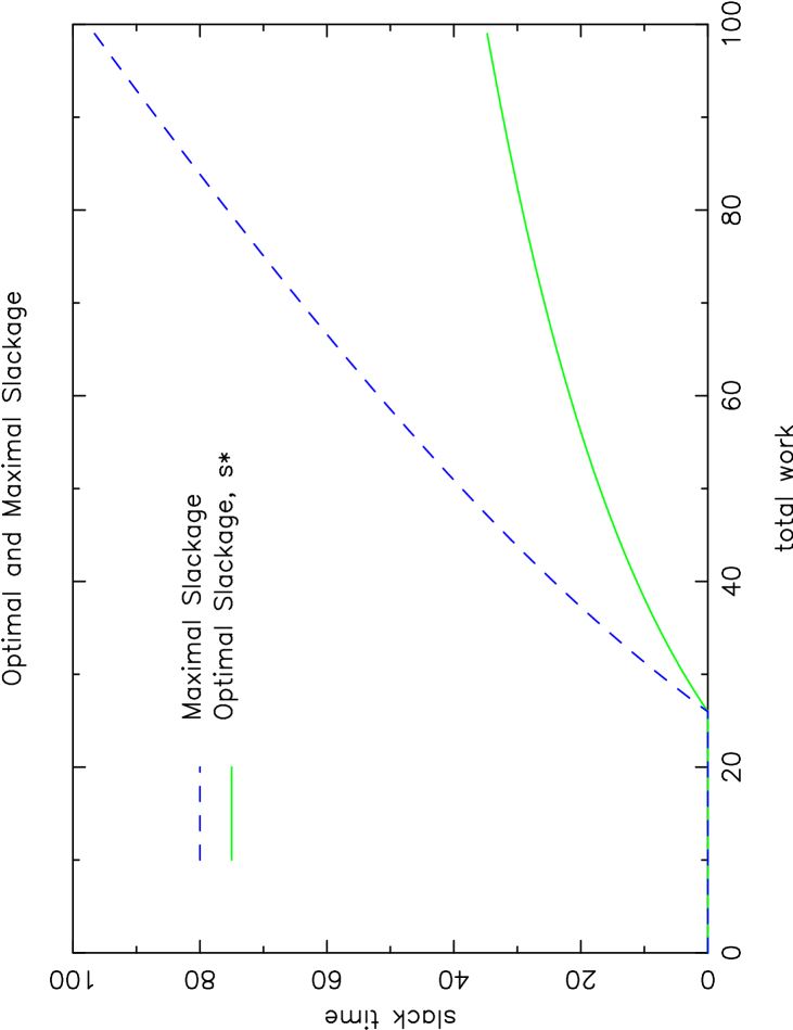
Figure 3:

This means that if we want to slack for a year, we should choose a task that would normally take 41.2 months to complete at current processor speeds. After our optimal year of goofing around we buy a new computer, put our noses to the grindstone, and finish the calculation $t_{c}$ months later, having saved ourselves 3.25 months worth of total time (plus having been able to slack for a year and honestly call it productive).

The time to optimally finish the task is simply given by substituting equation 7 into equation 3:

$$t\star=s\!\star+N(2^{-s\star/18})=t_{c}\left[1+\ln(N/t_{c})\right]$$ (8)

Figure 4:

The conclusion that is drawn from this is that simulations done with a $t_{c}$ (26 month) runtime on the best machine that can be purchased for a given cost when the calculation begins are indeed optimal in the sense of utilization of ever improving computer resources. They are the largest calculations that should be done with the present resources. The optimal time to begin any more arduous computation is in the future (after an optimal amount of slack time). Furthermore any more trivial calculation should have been started in the past because calculations smaller than $t_{c}$ months runtime complete in the order they are undertaken.

This suggests that for any given calculation there is a best time to start, and that a valid strategy would be to always attempt problems that optimally utilize the resources. Obviously the effect of Moore’s law is that that the optimal problem scales as the rate of computation. Our calculations place a normalization on this scale and suggest that you will get the best possible performance if you choose to attack problems that will take $t_{c}$ months to run on your computer when you get around to starting the computation.

References

Moore, G.E. 1965, Electronics (Volume 38 Number 8), pp. 114–117