VLA OH and H 1 ZEEMAN OBSERVATIONS
OF THE NGC 6334 COMPLEX

Abstract

We present OH and H 1 Zeeman observations of the NGC 6334 complex taken with the Very Large Array. The OH absorption profiles associated with the complex are relatively narrow ($\Delta\mbox{v}_{\rm FWHM}$ $\sim$ 3 km $\mbox{s}^{-1}$) and single-peaked over most of the sources. The H 1 absorption profiles contain several blended velocity components. One of the compact continuum sources in the complex (source A) has a bipolar morphology. The OH absorption profiles toward this source display a gradient in velocity from the northern continuum lobe to the southern continuum lobe; this velocity gradient likely indicates a bipolar outflow of molecular gas from the central regions to the northern and southern lobes. Magnetic fields of the order of 200 $\mu$G have been detected toward three discrete continuum sources in the complex. Virial estimates suggest that the detected magnetic fields in these sources are of the same order as the critical magnetic fields required to support the molecular clouds associated with the sources against gravitational collapse.

Sarma, et al. VLA OH and H 1 Zeeman Observations of the NGC 6334 complex

Received 1999 September 24; accepted 1999 November 24

1 INTRODUCTION

1.1 The Zeeman Effect and Magnetic Fields

The importance of magnetic fields in the star formation process is now widely acknowledged (e.g., [Mouschovias 1987]; [Shu, Adams, & Lizano 1987]; [Heiles et al. 1993]; [McKee et al. 1993]; [Crutcher 1999, hereafter C99]). The Zeeman effect in radio-frequency spectral lines is the only viable method for measuring the strength of the magnetic field in interstellar molecular clouds and star-forming regions. If the Zeeman splitting is smaller than the linewidth, only the line-of-sight component of the magnetic field can be measured; this is always the case for non-maser lines.

In this paper we discuss high spatial resolution Zeeman observations in OH and H 1 absorption toward the NGC 6334 complex. In the remainder of §1, we review some details of the complex; §2 contains details of the observations and reduction of the data. In §3, we present the results of our observations, and §4 contains discussions about these results.

1.2 The NGC 6334 Complex

NGC 6334 is a giant molecular cloud complex and star-forming region at a distance of 1.7 kpc ([Neckel 1978]). It lies about 0$\arcdeg$.5 above the galactic plane and extends $\sim$30$\arcmin$ parallel to it. The complex has been the subject of extensive studies at a variety of wavelengths. [Rodriguez, Canto, & Moran (1982, hereafter RCM82)] mapped the region at 6 cm wavelength with the VLA. They found six discrete continuum sources that lie along a ridge of radio emission parallel to the Galactic plane. Three of these sources had been known from previous single dish observations by [Schraml & Mezger (1969)]. RCM82 named these sources A to F, in order of increasing right ascension (Figures 1 & 2, this paper). [McBreen et al. (1979)] mapped the region with a 40$-$250 $\micron$ photometer and found six far infrared (FIR) sources. Of these, five lie along the ridge of radio emission; an additional weaker source lies further south. The FIR sources were labeled I through VI. Another continuum source, I(N), was seen at millimeter and submillimeter wavelengths ([Cheung et al.] 1978; [Gezari] 1982); I(N) lies to the north of FIR I and was not detected in the observations of [McBreen et al. (1979)]. [Dickel, Dickel, & Wilson (1977, hereafter DDW77)] detected four CO peaks within an extended region of emission. The nomenclature in this complex has become confused. In this paper, we adopt the convention of RCM82 for radio continuum sources.

Among the many phenomena associated with star formation in this complex are water masers ([Moran & Rodriguez 1980]), OH masers ([Gaume & Mutel 1987]), methanol masers ([Menten & Batrla 1989]), bipolar outflows in ionized and molecular gas ([De Pree et al.] 1995; [Bachiller & Cernicharo 1990]; [Phillips & Mampaso 1991]), and shocked $\mbox{H}_{2}$ emission ([Straw & Hyland 1989a]). Several authors have discussed a picture of sequential star formation in this complex ([Cheung et al.] 1978; [Moran & Rodriguez 1980]) in which the central parts of the complex are more evolved than the edges. This conclusion was mainly based on the distribution of indicators of star formation such as OH and $\mbox{H}_{2}\mbox{O}$ masers and CO, far-IR and 1 mm peaks. However, RCM82 point out that the picture is definitely more complex than simple sequential star formation. For example, source E, which lies at the edge of the complex, is an evolved source.

Table 1: Observational Parameters for VLA Observations

Parameter	H 1	OH
Date	1993 May 27	1996 Jan. 27
	1993 May 28
	1993 Oct. 22
Configuration	CnB, DnC	CnB
R.A. of field center (B1950)	$17^{h}$$17^{m}$$00^{s}$.0	$17^{h}$$17^{m}$$00^{s}$.0
Decl. of field center (B1950)	$-35$$45$$00$$.0$	$-35$$45$$00$$.0$
Total bandwidth (MHz)	0.78	0.19
No. of channels	128	128
Hanning smoothing	Yes	No
Channel Spacing (km $\mbox{s}^{-1}$)	1.28	0.27
Approx. time on source (hr)	12.6	4.3
Rest frequency (MHz)	1420.406	1665.402
		1667.359
FWHM of synthesized beam	35$\arcsec$ $\times$ 20$\arcsec$	16$\arcsec$ $\times$ 12$\arcsec$
rms noise (mJy $\mbox{beam}^{-1}$)
abcLine channels	10	8
abcContinuum	9	7

The NGC 6334 complex has also been the subject of extensive recent observational studies. [Kraemer et al. (1997, hereafter KJPB97)] and [Kraemer (1998a, hereafter K98)] observed the complex in transitions of CO, CS, and $\mbox{NH}_{\rm 3}$ and in ionized carbon and neutral oxygen ([C 2] 158 $\micron$, [O 1] 145 $\micron$, and [O 1] 63 $\micron$). They found that the molecular emission in NGC 6334 shows a complex structure of filaments and bubbles, some of which are filled with photodissociated gas ([Kraemer 1998b]). [Boreiko & Betz (1995, hereafter BB95)] observed the NGC 6334 complex in [C 2] 158 $\micron$ lines. They found that the C 2 radiation is bright and widespread, with a general correlation between regions of intense C 2 emission and warm dust and CO radiation.

2 OBSERVATIONS AND DATA REDUCTION

The observations were carried out with the Very Large Array (VLA) of the NRAO. The H 1 observations were carried out in 1993 in the CnB and DnC configurations. The OH observations were carried out in January 1996 in the CnB configuration. Table 1 lists the important parameters of the H 1 and OH observations. For H 1, both circular polarizations were observed simultaneously. For OH, both circular polarizations and both main lines (1665 and 1667 MHz) were observed simultaneously. In order to mitigate instrumental effects, a front-end transfer switch was used to reverse the sense of circular polarization received at each telescope every 10 minutes. Further, for the H 1 observations, all calibration sources were observed at frequencies displaced 1 MHz above and below the observing frequency for the source so that the Galactic H 1 emission would not affect the calibration. Roberts, Crutcher, & Troland (1995) describe very similar observational techniques applied to S106.

The editing, calibration, Fourier transformation, deconvolution, and processing of the H 1 and OH data were carried out using the Astronomical Image Processing System (AIPS) of the NRAO. Further processing of the data made use of the Multichannel Image Reconstruction, Image Analysis and Display (MIRIAD) system of the Berkeley-Illinois-Maryland Array (BIMA).

OH masers in the field of view can have significant effects upon the Zeeman analysis because they are often highly circularly polarized. Moreover, the effects of strong masers can be spread over the entire field of view in dirty maps owing to sidelobes of the synthesized beam. Successful removal of maser effects is only feasible if the data are very well calibrated. Only in this case is the actual response in the maps to a point source (e.g., a maser) equal to the calculated point source response function (the “dirty” beam). The problem of maser contamination is especially acute in the NGC 6334 region where there are two strong masers in the field. The strongest maser ($\sim$400 Jy) coincides with source F (Fig. 2), the next strongest ($\sim$50 Jy) lies within the shell-like region to the southwest of source A (§3.1; Fig. 2). There is also a weak maser at 1665 MHz ($\sim$1 Jy) on the western edge of source A (Fig. 4a). Fluxes given are the sum of right and left circular polarizations at 1665 MHz. To remove maser effects from the NGC 6334 OH data sets, we employed a several step process. First we performed a self calibration on the frequency channel with the strongest maser radiation. This channel is at a velocity of $-$8.8 km/s. Then we applied this self calibration solution to the entire dataset. Next we generated an image for each channel having maser radiation, and we specified boxes around each maser in the image. Within each box, we identified clean components that represented the maser radiation. Next we used the AIPS task UVSUB to compute and remove from the uv dataset the effects of these masers by using the clean components as the input model. Finally, we re-generated the images for each channel with the maser effects removed and combined these images with those of the other (non-maser affected) frequency channels.

3 RESULTS

3.1 Continuum

Figure 1 shows the 18 cm image of the discrete continuum sources in the NGC 6334 complex. Figure 2 shows the 21 cm grayscale continuum image of the entire complex, including the low-brightness shell-like sources in the extreme south that are not shown in Fig. 1. The 18 cm image has been made at higher resolution (12$\arcsec$ $\times$ 9$\arcsec$) by uniformly weighting the data. The compact radio continuum sources in this complex lie in a ridge that extends from the northeast to the southwest; there is an underlying bed of continuum which extends $\sim$5$\arcmin$ to the northwest of the ridge. The compact sources are labeled A$-$F, as described above (§1.2 and Fig. 1). RCM82 and [Rodriguez, Canto, & Moran (1988, hereafter RCM88)] have discussed the nature and morphology of these sources. RCM82 concluded that all the compact sources, with the exception of source B, are H 2 regions. [Moran et al. (1990)] have shown that B is extragalactic. For the compact sources, our estimates of the integrated fluxes are in reasonable agreement (within about 10$\%$) with RCM82, except for source E, where we obtain a flux of about 6 Jy, compared to their value of 12 Jy.

Figure 1: Contour image of the continuum sources in the NGC 6334 complex at 18 cm. Contour intervals are at 0.05, 0.1, 0.2, 0.4, 0.8, 1.6 Jy $\mbox{beam}^{-1}$. The beam is 12$\arcsec$ $\times$ 9$\arcsec$; the image has been made at a higher resolution by uniformly weighting the data. The rms in the image is 7 mJy $\mbox{beam}^{-1}$. Note that the two weak shell-like structures in the extreme south of NGC 6334, shown in Fig. 2, are not included in this figure.

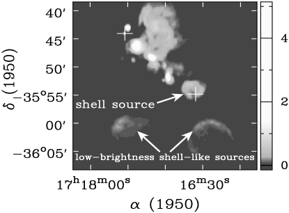
Figure 2: Grayscale radio continuum image of the entire NGC 6334 complex at 21 cm. The beam is 35$\arcsec$ $\times$ 20$\arcsec$, the rms in the image is 9 mJy $\mbox{beam}^{-1}$. The positions of the two strongest OH masers are marked by the white crosses; the northeastern OH maser coincides with source F. The shell-like source about 4$\arcmin$ to the southwest of source A is designated as “shell source” in this figure.

Figure 3: OH 1667 MHz optical depth profile toward (a) the northern lobe of source A at $\alpha$=$17^{h}$$16^{m}$$57^{s}$.8, $\delta$=$-$35$\arcdeg$51$\arcmin$09$\arcsec$; (b) the continuum peak of source A at $\alpha$=$17^{h}$$16^{m}$$57^{s}$.8, $\delta$= $-$35$\arcdeg$51$\arcmin$42$\arcsec$; and (c) the southern lobe of source A at $\alpha$=$17^{h}$$16^{m}$$57^{s}$.5, $\delta$= $-$35$\arcdeg$52$\arcmin$27$\arcsec$.

The bipolar morphology of source A (RCM 88) is clearly seen in the images (Fig. 1 and 4a). In their higher resolution 6 cm image, RCM88 also see a discontinuous shell in the core of the source. The weak unresolved source G351.24$+$0.65 to the east of source A was first discovered by [Moran et al. (1990)]; [De Pree et al.] (1995) concluded that this is an optically thin H 2 region. There is also a shell-like source about 4$\arcmin$ to the southwest of A (Fig. 1, 2; designated as “shell source” in Fig. 2). Parts of it coincide with the position of FIR source V. [Jackson & Kraemer (1999)] conclude that the relative distribution of ionized, photodissociated, and molecular gas (as seen in radio continuum, [C 2] 158 $\micron$, and CO 2$\rightarrow$1 emission respectively) toward this shell-like source conforms closely to an idealized model of a photodissociation region (PDR). In our 18 cm observations, the shell is almost complete, except for an opening in the south. An OH maser lies toward the south of this source, near the break in the shell (Fig. 2).

Of the other main sources in the NGC 6334 complex, source C is extended and has a nonspherical appearance in the 6 cm image of RCM82. There is a steep decrease in the continuum intensity toward the south of this source (Fig. 1). In both our 18 cm and 21 cm images, there is a low intensity source about 1$\arcmin$ to the south of C. Source D is extended, amorphous, and roughly spherical. Source E is also extended and spherical. Source F is unresolved in our observations. RCM82 found it to have a “nozzle-like” morphology with a sharp decrease in emission to the west and a smooth extension to the east. A very strong OH maser is coincident with the position of this source (§2; Fig. 2).

Two weak shell-like structures appear to the south of the star-forming ridge in NGC 6334 (Fig. 2, where they are marked as “low-brightness shell-like sources”). These two sources are coincident with the bright southern parts of the optical nebula of NGC 6334 ([Kraemer & Jackson 1999]). Also, part of the western shell-like source is coincident with the extended FIR source VI of [McBreen et al. (1979)]. Since the faint radio shells are seen as bright objects in the red plate of the Palomar Sky Survey, the extinction toward these shells must be very low.

3.2 OH & H 1 Absorption

Optical depth profiles for the OH and H 1 lines were calculated using the procedure described in [Roberts et al. (1995)]. These OH and H 1 profiles all contain a component at about $+$7 km $\mbox{s}^{-1}$ that likely arises in a foreground cloud. A cold H 1 cloud was observed at this velocity toward the Galactic center by [Riegel & Crutcher (1972)] and [Crutcher & Lien (1984)] and estimated to lie within 150 pc of the Sun. In all discussion that follows, we omit consideration of this foreground component and concentrate on negative velocity absorption that is associated with the NGC 6334 complex. The H 1 profiles generally consist of numerous blended velocity components extending to velocities as negative as $-$25 km $\mbox{s}^{\rm-1}$ (e.g., Fig. 6). The only exception to this rule is toward source C. In this case the H 1 profiles have a single relatively narrow component ($\Delta\mbox{v}_{\rm FWHM}$ $\sim$6 km $\mbox{s}^{\rm-1}$) centered at $-$6.6 km $\mbox{s}^{\rm-1}$.

The OH optical depth profiles have narrower less blended components with center velocities in the range $-$2 to $-$7 km $\mbox{s}^{-1}$. Their center velocities and linewidths are summarized in Table 2. We consider these components to be associated with the NGC 6334 complex based on CO and other molecular emission lines (DDW77; [De Pree et al.] 1995). Figure 3 shows the profiles in OH 1667 MHz toward the core and lobes of source A; the profiles toward this source exhibit a north-south velocity gradient of about 3.4 km $\mbox{s}^{\rm-1}$ $\mbox{pc}^{\rm-1}$. The H 1 absorption toward source A is saturated; velocity structure is more difficult to quantify. However, the H 1 profiles show evidence of a north-south velocity gradient similar to that in OH. We do not detect any OH absorption toward source C; however, detectable OH absorption is seen toward the low intensity continuum source about 1$\arcmin$ to the south of C. Considerable velocity structure is seen in OH absorption profiles over source D west of the continuum peak; we do not detect any OH absorption to the east of the continuum peak. Toward source E, the OH absorption profiles are single-peaked and broad toward the northeast of the source, and show two peaks toward the southwest.

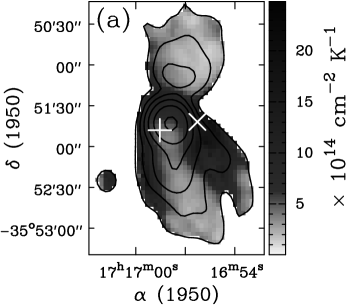
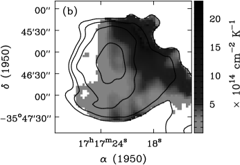
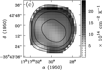
Figure 4: (a) Grayscale plot of N(OH)/$\mbox{T}_{\rm ex}$ toward source A in the NGC 6334 complex. The contours represent the naturally weighted 18 cm continuum, contours are at 0.1, 0.2, 0.4, 0.8, 1.6, 3.2 Jy $\mbox{beam}^{-1}$. The beam is 16$\arcsec$ $\times$ 12$\arcsec$. The ‘$+$’ represents the position at which we have measured the B-field. The ‘$\times$’ represents the position of the $\sim$1 Jy 1665 MHz maser on the western edge of source A. (b) Similar plot to (a), but toward source D. The contours are at 0.1, 0.2, 0.4, 0.8 Jy $\mbox{beam}^{-1}$. (c) Similar plot to (a), toward source E. The contours are at 0.1, 0.2, 0.4, 0.8 Jy $\mbox{beam}^{-1}$.

The OH column density was determined using the relation

$$\mbox{N}_{\rm OH}/\mbox{T}_{\rm ex}=\mbox{C}\int{{\tau}_{\rm v}\mbox{dv}}\phm{abc}\mbox{cm}^{\rm-2}\phm{b}\mbox{K}^{\rm-1}$$ (1)

where $\mbox{T}_{\rm ex}$ is the excitation temperature of OH and the constant C = $4.1063\times 10^{\rm 14}$ and $2.2785\times 10^{\rm 14}$ $\mbox{cm}^{-2}$ (km $\mbox{s}^{-1}$)^-1 for the OH 1665 and 1667 MHz lines respectively ([Crutcher 1977]). Figure 4 shows plots of N(OH)/$\mbox{T}_{\rm ex}$ toward sources A, D, and E in OH at 1667 MHz. In principle, variations in N(OH)/$\mbox{T}_{\rm ex}$ may arise due to variations in the OH column density, or due to variations in $\mbox{T}_{\rm ex}$, or both. However, in our results and discussion, we quote only variations in N(OH)/$\mbox{T}_{\rm ex}$, since the excitation temperature cannot be measured based on absorption studies alone. Further discussion about possible variations in $\mbox{T}_{\rm ex}$ appears in §4.2. Toward A, there is an increase in N(OH)/$\mbox{T}_{\rm ex}$ just north of the continuum peak in the core; this ridge of enhanced OH spans the source from east to west. Also, we observe an increase in N(OH)/$\mbox{T}_{\rm ex}$ along the eastern and western boundaries of the northern and southern lobes of source A. This effect is especially striking in the southern lobe. Toward source D, there is an increase in N(OH)/$\mbox{T}_{\rm ex}$ going west from the continuum peak (Fig. 4b) and no detectable OH absorption east of the continuum peak. N(OH)/$\mbox{T}_{\rm ex}$ is maximum in the northwestern part of this source. Toward source E, N(OH)/$\mbox{T}_{\rm ex}$ appears to increase from the center to the edge over most of the source (Fig. 4c). However, nothing definite can be said regarding the OH column density at the southeastern edge, where the information has been blanked in many channels to remove remnant effects of the strong maser in source F.

Finally, we note the absorption profiles toward some of the other positions in the NGC 6334 complex. Absorption in both OH and H 1 is seen toward the shell source to the southwest of A. OH absorption is seen toward the highest intensity patches in the north and west of this shell. The OH lines toward these regions have a $\Delta\mbox{v}_{\rm FWHM}$ $\sim$ 3 km $\mbox{s}^{-1}$ and are centered near $\mbox{v}_{\rm LSR}$ $\sim$ $-$6 km $\mbox{s}^{-1}$. Broad H 1 absorption profiles with several blended velocity components are also seen toward the two low-brightness shell-like sources in the extreme south of NGC 6334 (Fig. 2). Furthermore, OH and H 1 absorption is also seen toward some of the brighter regions of continuum emission to the northwest of source D.

ccccccccc 2 6 Observed features of line profiles & Position OH (1667 MHz)(a)
Source R.A. Decl. $\mbox{v}_{\rm LSR}$ $\Delta\mbox{v}_{\rm FWHM}$ (B1950) (B1950) (km $\mbox{s}^{-1}$) (km $\mbox{s}^{-1}$) A $17^{h}$$16^{m}$$57^{s}$.8 $-$35$\arcdeg$51$\arcmin$42$\arcsec$ $-$3.8 $\sim$3

C $17^{h}$$17^{m}$$10^{s}$.9 $-$35$\arcdeg$48$\arcmin$30$\arcsec$

S. of C $17^{h}$$17^{m}$$08^{s}$.1 $-$35$\arcdeg$49$\arcmin$24$\arcsec$ $-$2.5 $\sim$2

D $17^{h}$$17^{m}$$23^{s}$.0 $-$35$\arcdeg$46$\arcmin$15$\arcsec$ $-$5.8 $\sim$3

D $17^{h}$$17^{m}$$18^{s}$.7 $-$35$\arcdeg$46$\arcmin$39$\arcsec$ $-$4.7, $-$1.4 $\sim$3, $\sim$3

D $17^{h}$$17^{m}$$17^{s}$.0 $-$35$\arcdeg$46$\arcmin$51$\arcsec$ $-$3.0 $\sim$2

E $17^{h}$$17^{m}$$30^{s}$.5 $-$35$\arcdeg$42$\arcmin$57$\arcsec$ $-$5.5 $\sim$4

E $17^{h}$$17^{m}$$29^{s}$.3 $-$35$\arcdeg$43$\arcmin$15$\arcsec$ $-$6.9, $-$2.2 $\sim$3, $\sim$4

(a)All OH profiles also show a component at positive velocities which is not shown in this table; see §3.2 H 1 profiles show several blended velocity components between $-$25 and $+$14 km $\mbox{s}^{-1}$ toward all sources, except toward source C, where there are two components; one at the positive velocity mentioned in (a) above and the other is at $\mbox{v}_{\rm LSR}$ = $-$6.6 km $\mbox{s}^{-1}$ and $\Delta\mbox{v}_{\rm FWHM}$ $\sim$6 km $\mbox{s}^{-1}$

3.3 Magnetic Fields

Figure 5: (a) Stokes I (top-histogram) and V (bottom-histogram) profiles in the OH 1665 MHz line toward source A at the position marked by a ‘$+$’ in Fig. 4a, $\alpha_{\rm 1950}$ = $17^{h}$$16^{m}$$58^{s}$.5, and $\delta_{\rm 1950}$ = $-$35$\arcdeg$51$\arcmin$48$\arcsec$. The continuous line superposed on the V spectrum in the lower box is the derivative of I scaled by the derived value of $\mbox{B}_{\rm los}$ = 148 $\mu$G. (b) Same as (a), but for OH 1667 MHz, and a derived value of $\mbox{B}_{\rm los}$ = 162 $\mu$G.

To determine magnetic field strengths using the Zeeman effect, we fitted a numerical derivative of the Stokes I spectrum to the Stokes V spectrum for each pixel in the absorption line cube. The technique is described in [Roberts et al. (1993)]. The results of the fits, which give the line-of-sight component of the magnetic field, $\mbox{B}_{\rm los}$, toward the various sources in the complex are listed in Table 3. We consider the results to be significant if the derived value of $\mbox{B}_{\rm los}$ is greater than the 3$\sigma$ level. For OH, we have imposed a stronger condition $-$ the results are considered significant only if $\mbox{B}_{\rm los}$ is greater than the 3$\sigma$ level for both 1665 and 1667 MHz lines. Field values that we believe to be significant are shown in bold face type in the table. In OH, significant detections of the magnetic field were made toward source A. In H 1, significant detections of the magnetic field were made toward source E and source D. Figure 5 shows the Stokes I and V profiles toward the core of source A (the position marked with a ‘$+$’ in Fig. 4a) in the 1665 and 1667 MHz lines of OH, together with the derivative of the I profile scaled by the fitted value of the magnetic field. Figure 6 shows the Stokes I and V profiles and the scaled derivative of the I profile in H 1 toward source E. By convention, a positive value of $\mbox{B}_{\rm los}$ indicates that the field is pointing away from the observer.

crrrrrrrrr 3 8 Magnetic Field Values Position OH H 1 Source R.A. Decl. 1665 MHz 1667 MHz 1420 MHz A $17^{h}$$16^{m}$$58^{s}$.5 $-$35$\arcdeg$51$\arcmin$48$\arcsec$ 148$\pm$20 162 $\pm$33 47$\pm$15 D $17^{h}$$17^{m}$$22^{s}$.2 $-$35$\arcdeg$46$\arcmin$21$\arcsec$ $-$60$\pm$46 $-$69$\pm$58 $-$93$\pm$13 E $17^{h}$$17^{m}$$30^{s}$.1 $-$35$\arcdeg$43$\arcmin$09$\arcsec$ $-$263$\pm$78a $-$340$\pm$78a $-$169$\pm$33 $-$180$\pm$29b NW of D $17^{h}$$17^{m}$$08^{s}$.6 $-$35$\arcdeg$42$\arcmin$29$\arcsec$ 169$\pm$55

afrom OH data convolved with 35$\arcsec$ beam bfrom H 1 data convolved with a 35$\arcsec$ circular beam for comparison with OH results values in boldface type are significant detections (see §3.3)

Figure 6: Stokes I (top-histogram) and V (bottom-histogram) profiles in the H 1 line toward source E at the position $\alpha_{\rm 1950}$ = $17^{h}$$17^{m}$$30^{s}$.1, and $\delta_{\rm 1950}$ = $-$35$\arcdeg$43$\arcmin$09$\arcsec$. The continuous line superposed on the V spectrum in the lower box is the derivative of I scaled by the derived value of $\mbox{B}_{\rm los}$ = $-$169 $\mu$G.

Toward source A, the OH data provide some tentative indications of field strength variations. Field strengths in the 1667 MHz line increase by a factor of two or more to the north of the continuum peak, in the direction of the east-west ridge of enhanced OH optical depth (Fig. 4a). However, weak maser contamination in this ridge at 1665 MHz prevented us from confirming this result in the 1665 MHz line. This maser coincides in velocity with one side of the absorption line, and its effect in the Stokes V profile cannot be removed completely. We can, of course, exclude the channels contaminated by the maser from the fit, and compare the values of the magnetic field in 1665 and 1667 MHz. However, higher resolution OH data will be needed to investigate such variations anyway since the existing data provide only three to four independent resolution elements across source A. Therefore, we defer examination of the spatial variation of the magnetic field in source A to a later higher resolution study.

Toward source E, where we have a significant detection in H 1, we also find a possible detection in the 1665 and 1667 MHz absorption lines of OH. Our maser removal process has diminished the effect of the masers to a large extent. However, it has proved impossible to completely remove the effect of the strong maser in source F in the Stokes V profile in a region so close to the maser. Therefore, in fitting for the magnetic field in source E, we have fitted over only those channels in the absorption line that are not affected by the maser. To improve our noise estimates, we have convolved our OH data with a 35$\arcsec$ beam. For comparison, we also convolved the H 1 data with a circular 35$\arcsec$ beam. Magnetic field values in the 1665 and 1667 MHz OH data are consistent, and the H 1 data reveal a significant field of similar order and the same sign. Finally, there is also a possible detection in H 1 toward an area of continuum to the northwest of source D. This fit is barely at the 3$\sigma$ level, so we state it as an upper limit. If it is real, it represents a reversal in the sign of the field in going from the region near D and E to the region northwest of D.

4 DISCUSSION

4.1 Individual Sources in the NGC 6334 Complex

4.1.1 Source A

The morphology of continuum emission from this source, including its bipolar structure, has been described in §1.1. The peak of the FIR source IV lies near the peak of the radio source. Also associated with source A are a Herbig-Haro-like object ([Gyulbudaghian, Glushkov, & Denisyuk 1978]; [Bohigas 1992]), $\mbox{H}_{\rm 2}\mbox{O}$ masers ([Rodriguez et al. 1980]; [Moran & Rodriguez 1980]), and a CO peak (DDW77; [Phillips, de Vries, & de Graauw 1986, hereafter PVG86]; K98). RCM88 suggested that the bipolar morphology of this region results from the confinement of the H 2 region by a flattened structure of gas and dust. This east-west confinement allows the ionized gas to escape only to the north and south. Indeed, a 40$\arcsec$ resolution map of 100 $\micron$ optical depth from [Harvey & Gatley (1983)] shows an east-west elongation, which suggests a flattened structure of dust with an east-west extent of at least 100$\arcsec$. Their map center coincides with the center of the ridge of enhanced N(OH)/$\mbox{T}_{\rm ex}$ in our data (§3.2 and Fig. 4a). The east-west ridge of enhancement in our OH optical depth may be related to this disk. KJPB97 observed various transitions of CO and CS toward source A (HPBW of CO J=1$\rightarrow$0 observations = 53$\arcsec$). Their data show that source A is surrounded by a 4$\arcmin$.4 $\times$ 1$\arcmin$.8 structure, indicating that the molecular cloud is also flattened on much larger scales.

The kinematical data for source A and its environs also offer insights into the physical nature of this region. On the larger scale of 4$\arcmin$ (2 pc), KJPB97 find an east-west velocity gradient of 2.4 km $\mbox{s}^{\rm-1}$ $\mbox{pc}^{\rm-1}$ in the gas traced by CO and CS. They conclude that a rotating disk of molecular gas surrounds source A. Our OH absorption data also reveal an east-west velocity gradient of the same sign. Over a 35$\arcsec$ (0.3 pc) scale size, this gradient amounts to 4 km $\mbox{s}^{\rm-1}$ $\mbox{pc}^{\rm-1}$. [De Pree et al.] (1995) have observed ionized and neutral gas (H76$\alpha$ and H92$\alpha$ recombination lines, and $\mbox{H}_{\rm 2}$CO absorption) toward source A with a resolution of about 5$\arcsec$. They report some indications of east-west velocity gradients in the opposite sense of those cited above. KJPB97 have noted the disagreement between the sense of rotation as conveyed by their molecular data, and [De Pree et al.] (1995)’s recombination line and $\mbox{H}_{\rm 2}$CO absorption data. However, our OH data agree in sign with KJPB97’s data over a larger scale size. The velocity gradients seen by [De Pree et al.] (1995) over smaller size scales (about 15$\arcsec$) may, therefore, reflect local velocity inhomogeneities in the core of the source, rather than any bulk rotation in the east-west direction.

Evidence for north-south motions in the bipolar lobes comes from two sources. [De Pree et al.] (1995) detect a north-south velocity gradient in H92$\alpha$ over a size scale of 100$\arcsec$, amounting to 19 km $\mbox{s}^{\rm-1}$ $\mbox{pc}^{\rm-1}$. They conclude that this indicates a bipolar outflow of ionized gas into the northern and southern lobes from the central source. They argue that this outflow lies nearly in the plane of the sky, based on the extended bipolar morphology and small velocity gradient. Our OH absorption data (§3.2 and Fig. 3) reveal a north-south gradient of 3.4 km $\mbox{s}^{\rm-1}$ $\mbox{pc}^{\rm-1}$ over a size scale of 80$\arcsec$. This suggests that the molecular gas traced by OH absorption is also part of an outflow from the central regions to the northern and southern lobes. This north-south velocity gradient in OH has the same sign as the north-south gradient in H92$\alpha$ detected by [De Pree et al.] (1995). This correspondence in sign suggests that the OH gas may lie close to the neutral-ionized interface and be entrained by the outflow of the ionized gas.

The [C 2] 158 $\micron$ profile of BB95 (HPBW = 43$\arcsec$) toward FIR IV shows two peaks near $-$1 km $\mbox{s}^{-1}$ and $-$5 km $\mbox{s}^{-1}$. BB95 note, however, that their spectra cannot be fitted by two Gaussian emission components. They mention a feature toward FIR IV with a velocity near $-$3 km $\mbox{s}^{-1}$ which is apparently due to self-absorption. We convolved our OH data with a 43$\arcsec$ beam for comparison with their data. Toward the position of FIR IV in source A, our OH profiles show an absorption feature near $-$3.7 km $\mbox{s}^{-1}$. Therefore, our data support the idea that the minimum between $-$1 and $-$5 km $\mbox{s}^{-1}$ in the [C 2] 158 $\micron$ profile is, indeed, self-absorption. The CO profiles of DDW77 and PVG86 also show a peak near $-$3 km $\mbox{s}^{-1}$ toward FIR IV, and a $\Delta\mbox{v}_{\rm FWHM}$ $\sim$ 7 km $\mbox{s}^{-1}$.

A significant $\mbox{B}_{\rm los}$ ($\sim$ 150 $\mu$G) was detected in OH 1665 and 1667 MHz absorption toward source A. We note that the magnetic field obtained from the formal fit in H 1 is of the same order although less than the magnetic field detected in OH. Due to the blending in velocity in the H 1 gas, it is almost certain that optical depth effects will suppress any Zeeman signature in the V profile ([Schwarz et al. 1986]), which may explain why we do not have a more significant detection of $\mbox{B}_{\rm los}$ in H 1 toward source A.

4.1.2 Source D

The extended, featureless source D (Fig. 4b) coincides with the FIR peak II of [McBreen et al. (1979)] and an $\mbox{H}_{\rm 2}\mbox{O}$ maser ([Moran & Rodriguez 1980]). Based on their 6 cm radio continuum measurements, RCM82 found that a ZAMS O6.5 star would be required to ionize this H 2 region. [Straw, Hyland, & McGregor (1989)] found that IRS 24, which lies close to the center of the continuum source and has a dereddened K magnitude corresponding to a ZAMS O6 star, is the dominant source of excitation in this source. Source D is located at the edge of a hole in the molecular gas emission, as seen in K98’s CO data. Their models suggest that the molecular hydrogen column density toward source D is the lowest of any source in the NGC 6334 complex. [Straw & Hyland (1989b)] used near-infrared star counts to find the extinction through NGC 6334; their estimates also suggest that the extinction toward source D is less than that toward any other sources. This hole in the molecular gas emission is clearly reflected in our high resolution image of source D (Fig. 4b), where no OH absorption is detected east of the continuum peak.

BB95 model their C 2 profile toward FIR I (source F) as an emission component centered at $\mbox{v}_{\rm LSR}$ = $-$5.2 km $\mbox{s}^{-1}$ and an absorption component near $\mbox{v}_{\rm LSR}$ = $-$1.6 km $\mbox{s}^{-1}$, and note that the source of the absorbing gas at this velocity is unclear. This absorption feature is also found near FIR II (toward source D). The CO profiles nearest to FIR II (of DDW77 with a 70$\arcsec$ beam and of PVG86 with a 1$\arcmin$.7 beam) are broad ($\Delta\mbox{v}_{\rm FWHM}$ $\sim$ 7 km $\mbox{s}^{-1}$) but appear to be Gaussian and single-peaked near $-$3 km $\mbox{s}^{-1}$. Our OH absorption profiles in this region show considerable velocity structure (§3.2). However, when convolved with a 43$\arcsec$ beam, our OH spectra show two components near $\mbox{v}_{\rm LSR}$ $\sim$ $-$5.0 and $-$1.6 km $\mbox{s}^{-1}$. This result suggests that both C 2 velocity components identified by BB95 lie on the near side of the H 2 region source D.

4.1.3 Source E

Source E is the northernmost compact radio continuum source in NGC 6334. RCM82 found that a ZAMS O7.5 star would be required to produce this H 2 region. [Tapia, Persi, & Roth (1996)] detected at least 12 faint K-band sources toward source E; these sources were not detected in the J- or H-bands. They suggested that these are a cluster of B0-B0.5 ZAMS stars which collectively ionize the H 2 region.

The C 2 profile of BB95 closest to source E is the one 1$\arcmin$ northwest of FIR I. The profile displays a peak near $\sim$ $-$8 km $\mbox{s}^{-1}$, and a lower level wing extends up to $\sim$ $+$2 km $\mbox{s}^{-1}$. Interestingly enough, the OH absorption profile toward the north of source E, when convolved with a 43$\arcsec$ beam for comparison with BB95’s data, is almost identical to this C 2 profile in shape and extent, except that the peak of the absorption is at $-$6.6 km $\mbox{s}^{-1}$. The H 1 absorption is present at all these velocities.

4.2 Virial Estimates

A principal goal of Zeeman effect measurements is to estimate the importance of the magnetic field to the dynamics and evolution of star forming regions like NGC 6334. Such estimates also require that other physical parameters of the regions be known, such as internal velocity dispersion, proton column density, radius, and total mass. C99 has summarized these concepts. Here, we apply such a simple analysis of magnetic effects to NGC 6334 sources A, E, and D, especially source A for which physical quantities are best known.

cc 4 Source A Parameters Parameter Value Radius (r) 0.8 pc Mass (M) 2200 $\mbox{M}_{\rm\odot}$ $\mbox{N}_{\rm{H_{\rm 2}}}$ 4.8 $\times$ ${\rm 10}^{\rm 22}$ $\mbox{cm}^{-2}$ $\mbox{n}_{\rm p}$ 3 $\times$ ${\rm 10}^{\rm 4}$ $\mbox{cm}^{-3}$ $\mbox{T}_{\rm k}$ 40 K $\Delta$v 2.6 km $\mbox{s}^{\rm-1}$ $\mbox{B}_{\rm los}$ 150 $\mu$G

First, we must estimate other relevant physical parameters. Column densities can be estimated from molecular line data such as that reported here, subject to several assumptions. For source A, we estimate column densities from our own OH data. We use an average value of N(OH)/$\mbox{T}_{\rm ex}$ equal to 6 $\times$ $10^{14}$ $\mbox{cm}^{\rm-2}$ $\mbox{K}^{\rm-1}$ to calculate N(OH) toward this source. The excitation temperature cannot be measured based on absorption studies alone. We adopt $\mbox{T}_{\rm ex}$ = 40 K. K98 found $\mbox{T}_{\rm k}$ = 50 K toward source A based on CO studies. [Forster et al. (1987)] found $\mbox{T}_{\rm k}$ $\sim$ 40 K from their ammonia studies. It is unlikely that $\mbox{T}_{\rm ex}$ remains constant over this source, and it may vary down to the dark cloud value of 10 K in the densest parts of the source. However, the results will scale with the temperature. The conversion ratio $\mbox{N}_{\rm{H_{\rm 2}}}$/N(OH)=2 $\times$ $10^{\rm 6}$ was taken from [Roberts et al. (1995)] for S106. This ratio is an order of magnitude higher than the ratio for dark clouds determined by [Crutcher (1979)]. However, we find N(OH)/$\mbox{A}_{\rm v}$ $\sim$ 5 $\times$ $\mbox{10}^{\rm 14}$, where we have used $\mbox{A}_{\rm v}$ = 50 mag., based on PVG86’s estimate of $\mbox{A}_{\rm v}$ $\sim$ 40 mag. toward a position about 1$\arcmin$ to the southeast of A. Using the standard conversion ratio of $\mbox{N}_{\rm{H_{\rm 2}}}$/$\mbox{A}_{\rm v}$ $\sim$ ${\rm 10}^{\rm 21}$, we obtain $\mbox{N}_{\rm{H_{\rm 2}}}$/N(OH) $\sim$ 2 $\times$ $10^{\rm 6}$ in agreement with [Roberts et al. (1995)], which justifies our use of the [Roberts et al. (1995)] value rather than the dark cloud value. Using this conversion ratio, we obtain a value of $\mbox{N}_{\rm{H_{\rm 2}}}$ = 4.8 $\times$ $\mbox{10}^{\rm 22}$ $\mbox{cm}^{\rm-2}$. Note that this value compares well with the value of $\mbox{N}_{\rm{H_{\rm 2}}}$= 1.3 $\times$ $\mbox{10}^{\rm 23}$ $\mbox{cm}^{\rm-2}$ obtained by KJPB97 based on their CO excitation models, and with K98’s value of 8.9 $\times$ $\mbox{10}^{\rm 22}$ $\mbox{cm}^{\rm-2}$ based on CO integrated intensity. Next, the most problematic parameter is the radius of the molecular cloud. K98 report a range of values for the radius based on their CO and CS emission studies. Using the average value of $\mbox{N}_{\rm{H_{\rm 2}}}$ = 4.8 $\times$ $\mbox{10}^{\rm 22}$ $\mbox{cm}^{\rm-2}$ and different values for the radius, we estimated the mass and proton density toward source A. The best value of the radius was then taken to be that for which the mass of the molecular cloud most closely matched the mass obtained by KJPB97 from their CO data. Further, this adopted value of the radius (0.8 pc) matches well with the radius of the molecular cloud in ${}^{\rm 13}\mbox{CO}$ 2$\rightarrow$1 (0.8 pc) and CS 3$\rightarrow$2 (0.7 pc) from KJPB97. Results of our analysis for source A are given in Table 4. Note that our value for the proton density is $\sim$ 2 higher than their value. For source E, where some of the above parameters are not available, we adopt a value of $N_{\rm{H_{\rm 2}}}$ = 6.3 $\times$ $10^{\rm 22}$ $\mbox{cm}^{\rm-2}$ from K98, as derived from CO excitation model calculations. Similarly, for source D, we use their value of $N_{\rm{H_{\rm 2}}}$ = 2.2 $\times$ $10^{\rm 22}$ $\mbox{cm}^{\rm-2}$.

The most straightforward estimate of the importance of the magnetic field comes from the relation :

$$\mbox{B}_{\rm S,crit}=5\times{10^{\rm-21}\phm{b}\mbox{N}_{\rm p}}\phm{abc}\mu\mbox{G}$$ (2)

where $\mbox{N}_{\rm p}$ is the average proton column density of the cloud, and $\mbox{B}_{\rm S,crit}$ is the average static magnetic field in the cloud that would completely support it against self gravity. Note that the magnetic field in a cloud can be described in terms of a static component $\mbox{B}_{\rm S}$, and a time-dependent component $\mbox{B}_{\rm W}$. It is likely that the Zeeman effect primarily samples the static component (see [Brogan et al. 1999], and references therein). If the actual field in the cloud is comparable to $\mbox{B}_{\rm S,crit}$, then the field can be judged dynamically important to the region. For source A, we find $\mbox{B}_{\rm S,crit}$ = 500 $\mu$G, compared to an estimated total field strength of 300 $\mu$G. Following C99, we have used total magnetic field strength B equal to 2 times $\mbox{B}_{\rm los}$, and $\mbox{$|$B$|$}^{\rm 2}$ equal to 3 times ${|\mbox{B}_{\rm los}}|^{\rm 2}$. For source E, we find $\mbox{B}_{\rm S,crit}$ = 600 $\mu$G, compared to an estimated total field strength of 400 $\mu$G. Again, for source D, we find $\mbox{B}_{\rm S,crit}$ = 220 $\mu$G, compared to an estimated total field strength of 190 $\mu$G. Therefore, subject to the obvious uncertainties in such estimates, we judge the magnetic field in each region to be comparable to if slightly less than the critical field. In all three regions, the magnetic field should be dynamically significant, providing an important source of support against self gravity.

cc 5 Source A : Derived Values and Virial Estimates Parameter Value $\sigma$/c 2.9 $\sigma$/$\mbox{v}_{\rm A}$ 0.3 $\mbox{$\beta$}_{\rm p}$ 0.03 ${[\mbox{M}/{{\Phi}_{\rm B}}]}_{obs/crit}$ 1.6 $\cal{W}$ 3.7 $\times$ ${\rm 10}^{\rm 47}$ ergs $\cal{T}$/$\cal{W}$ 0.22 $\cal{M}$/$\cal{W}$ 0.27

$\sigma$ is the line velocity dispersion, c is the speed of sound, $\mbox{v}_{\rm A}$ is the Alfvén velocity, $\mbox{M}/{{\Phi}_{\rm B}}$ is the mass to magnetic flux ratio, $\cal{W}$ is the virial gravitational energy, $\cal{T}$ is the virial kinetic energy, and $\cal{M}$ is the virial magnetic energy; all terms are defined in C99.

Other parameters of magnetic significance for source A can be inferred from the data of Table 4; they are shown in Table 5. All symbols used in the discussion that follows are described in Table 5. We find $\sigma$/c =2.9, indicating that the motions in the cloud are supersonic. This is a common result in molecular clouds; C99 has found that motions are supersonic by about a factor of 5. However, the ratio $\sigma$/$\mbox{v}_{\rm A}$ indicates that they are sub-Alfvénic, suggesting that these motions may be the result of Alfvén waves in the cloud. The parameter ${\rm\beta}_{\rm p}$ $\approx$ 0.03, close to the average value of 0.04 determined by C99, suggesting that the magnetic fields are important, and that the magnetic pressure dominates over the thermal pressure. The observed mass-to-magnetic flux ratio with respect to the critical value is 1.6, indicating that the cloud is magnetically supercritical. Also, $\cal{T}$ $\approx$ $\cal{M}$. Thus, the kinetic and magnetic energy densities are in approximate equilibrium, which would be expected if the magnitude of the fluctuating part of the magnetic field was approximately equal to the magnitude of the static field (C99). Finally, we find that 2$\cal{T}$ $+$ $\cal{M}$ $\approx$ 0.7$\cal{W}$. Hence, since the external pressure term, which is not included here, will act in the same sense as the gravitational term, the cloud is in approximate virial equilibrium.

5 CONCLUSIONS

1). We have observed OH and H 1 in absorption toward NGC 6334 with the VLA. The OH absorption profiles are relatively narrow ($\Delta\mbox{v}_{\rm FWHM}$ $\sim$ 3 km $\mbox{s}^{-1}$) and single-peaked toward most of the sources. Toward source A, the OH profiles display an east-west velocity gradient; this gradient has the same sign as the velocity gradient detected in molecular emission lines by KJPB97. The OH profiles toward source A also display a north-south velocity gradient which is in agreement with a similar gradient discovered in H92$\alpha$ recombination lines, and which likely indicates a bipolar outflow of material into the lobes seen in the continuum source. No OH absorption is detected toward the continuum peak of source C itself. Toward source D, the OH profiles show considerable velocity structure west of the continuum peak; no OH absorption is detected east of the continuum peak. The H 1 profiles toward NGC 6334 contain several blended velocity components, except toward source C, where the H 1 profile at negative velocities is almost single-peaked.

2). We have calculated N(OH)/$\mbox{T}_{\rm ex}$ toward the continuum sources. Toward source A, we observe an increase in N(OH)/$\mbox{T}_{\rm ex}$ in an east-west ridge north of the continuum peak; there is also an increase toward the eastern and western boundaries of the northern and southern lobes.

3). Magnetic fields of the order of 200 $\mu$G have been detected toward some of the sources in this complex. In OH, we have significant detections of magnetic fields toward source A, and possibly a significant detection toward source E. In H 1, we have significant detections toward sources E and D. There may also be a detection toward an area of continuum to the northwest of source D. Also, $\mbox{B}_{\rm los}$ obtained from the formal fit for source A in H 1 is of the same order as $\mbox{B}_{\rm los}$ detected in OH absorption toward source A; similarly, $\mbox{B}_{\rm los}$ obtained from the formal fit for source D in OH matches $\mbox{B}_{\rm los}$ detected in H 1 absorption toward this source.

4). We have three or four independent beams across source A; measurements at different positions in 1667 MHz suggest that the magnetic field increases going north of the continuum peak. The signs of the detected magnetic fields are opposite in going from sources E and D (where we have a detection in H 1 absorption) to source A (where we have a detection in OH). If the field detected in H 1 to the northwest of D is real, there is also a sign reversal in the field in going from D and E to the position northwest of D.

5). We have used various observed and derived parameters to study the implications of the detected magnetic fields toward sources A, E, and D. In all cases, it appears that the detected fields are of the order of the critical field needed to support the molecular cloud associated with that source against gravitational collapse. We have also compared various derived parameters for source A with the published values of those parameters determined from an ensemble of clouds by C99.