Two Stellar Mass Functions Combined into One by the Random Sampling Model of the IMF

Abstract

The turnover in the stellar initial mass function (IMF) at low mass suggests the presence of two independent mass functions that combine in different ways above and below a characteristic mass given by the thermal Jeans mass in the cloud. In the random sampling model introduced earlier, the Salpeter IMF at intermediate to high mass follows primarily from the hierarchical structure of interstellar clouds, which is sampled by various star formation processes and converted into stars at the local dynamical rate. This power law part is independent of the details of star formation inside each clump and therefore has a universal character. The flat part of the IMF at low mass is proposed here to result from a second, unrelated, physical process that determines only the probability distribution function for final star mass inside a clump of a given mass, and is independent of both this clump mass and the overall cloud structure. Both processes operate for all potentially unstable clumps in a cloud, regardless of mass, but only the first shows up above the thermal Jeans mass, and only the second shows up below this mass. Analytical and stochastic models of the IMF that are based on the uniform application of these two functions for all masses reproduce the observations well.

1 Introduction

Recent theoretical models suggest that the stellar initial mass function may result from star formation in hierarchically-structured, or multifractal clouds that are characterized by a local conversion time of gas into stars that is everywhere equal to the dynamical time on the corresponding mass scale (Elmegreen 1997, 1999a, hereafter papers I and II). This model gives the Salpeter power law slope, which was suggested to be the best representation of the IMF at intermediate to high mass (see reviews of observations in Scalo 1986, 1998; papers I, II, and Massey 1998), and it gives a break from that slope to a flattened or possibly decreasing part at lower mass where interstellar clumps cannot become self-gravitating during normal cloud evolution. This break point may be at the thermal Jeans mass, given by the Bonner-Ebert critical mass

$$M_{J}=0.35\left({{T}\over{10K}}\right)^{2}\left({{P}\over{10^{6}\;k_{B}}}\right)^{-1/2}\;\;{\rm M}_{\odot}$$ (1)

for temperature $T$ and total pressure $P$ (thermal + turbulent + magnetic) in the star-forming region.

The thermal Jeans mass is fairly constant from region to region in normal galaxies (Paper II), or at least as constant as the IMF is observed to be, considering the limited data on the low-mass flattened part. Yet the characteristic mass $M_{J}$ may be varied, if needed, to account for a high mass bias in starburst regions (Rieke et al. 1980) or the early Universe (Larson 1998) if $T^{2}$ increases more than $P^{1/2}$. Such a change might be expected in high density regions because they have more intense and concentrated star formation.

A general lack of understanding of the details of star formation during the final stages has limited the success of the model so far to the power law range, and to all of the implications of stochastic, rather than parameterized, star formation (Papers I and II). The low mass part of the IMF had not been observed well anyway, so the original models made no effort to fit any data there.

There is a growing consensus, however, that the low mass IMF becomes approximately flat (slope=0) over a significant range in mass when plotted as a histogram of the log of the number of stars per unit logarithmic mass interval versus the log of the mass. In such a plot, the Salpeter (1955) slope is $-1.35$. This flattening was suspected over two decades ago (Miller & Scalo 1979), but the most recent observations are much clearer (Comeron, Rieke, & Rieke 1996; Macintosh, et al. 1996; Festin 1997; Hillenbrand 1997; Luhman & Rieke 1998; Cool 1998; Reid 1998; Lada, Lada & Muench 1998; Hillenbrand & Carpenter 1999).

As a result of these new observations, we suspect that the physical origin of the low mass IMF can be understood in statistical terms to the same extent as the power law part. This paper offers one possible explanation for the flattening of the IMF at low mass that may be easily tested with modern observations of star formation in resolved clumps. This explanation is made here after first reviewing the origin of the power law part of the IMF at intermediate to high mass.

2 The Random Sampling Model

Diffuse interstellar clouds and the pre-star formation parts of self-gravitating clouds are generally structured in a hierarchical fashion with small clumps inside larger clumps over a wide range of scales (see reviews in Scalo 1985; Elmegreen & Efremov 2000; for a review of cloud fractal structure, see Stützki 1999). Stellar masses occur in the midst of this clump range, neither at the smallest nor the largest ends, and there is no distinction in the non-self-gravitating (pre-stellar) clump spectrum indicating where the stellar mass spectrum will eventually lie. These observations imply that the basic environment for star formation is scale-free, so the mass scale for stars has to come from specific physical processes. In papers I and II, we proposed that the mass scale arises because of the need for self-gravity to dominate the most basic of all forces, thermal pressure, and this leads to the $M>M_{J}$ constraint discussed above. In fact, the break point in the power law part of the IMF arises at about $M_{J}$ for normal conditions.

The Salpeter power-law portion of the IMF was then proposed to arise as stars form out of gas structures that lie at random levels in the hierarchy (where $M>M_{J}$). Perhaps the physical process that initiates this is turbulence compression followed by gravitational collapse of the compressed slab (Elmegreen 1993; Klessen, Heitsch, & MacLow 2000), or perhaps it is an external compression acting on a certain gas structure. Regardless, the star formation process samples the hierarchical structure of the cloud in this model, and builds up a stellar mass spectrum over time.

This process of sampling where and when a particular star forms can only be viewed as random at the present time, just as the time and place of rain in a terrestrial cloud pattern is random and given only as a probability in most weather forecasts. The detailed star formation processes are not proposed to be random, only the manifestation of them, considering that turbulence is too complex for initial and boundary conditions to be followed very far over time and space with enough certainty to produce a predictable result. Thus we discuss here and in the previous two papers only the probability of sampling from various hierarchical levels, and we use this probability to generate a stochastic model that builds up the IMF numerically after many random trials. From this point of view, the basic form of the IMF is fairly easy to understand, even though the final slope has not been derived analytically (i.e., it has been obtained only by running the computer model).

For example, if the sampling process has a uniform probability over all hierarchical levels, then the mass spectrum is $M^{-2}dM=M^{-1}d\log M$ exactly (e.g., Fleck 1996; Elmegreen & Falgarone 1996). A dynamically realistic cloud will not sample in such a uniform way, however. It will be biased towards regions of higher density as they evolve more quickly. For most dynamical processes that precede star formation, including self-gravitational contraction, magnetic diffusion, and turbulence, the rate of evolution scales with the square root of the average local density. This means that lower mass clumps are sampled more often than higher mass clumps. As a result, the mass spectrum steepens to $M^{-1.15}d\log M$. The extra $-0.15$ in the power comes from $(D-3)/2D$ for fractal dimension $D$ (Paper I).

In addition to this steepening from density weighting, there is another steepening effect from mass competition. Once a small mass clump turns into an independent, self-gravitating region, the larger mass clump that surrounds it has less gas available to make another star. If it ever does make a star, then the mass of this star will be less than it would have been if the first star inside of it had never formed. After these two steepening effects, the IMF becomes $M^{-1.35}d\log M$, which is the Salpeter function.

3 The Flat Part of the IMF

The process of random, weighted sampling from hierarchical clouds changes below the thermal Jeans mass because most of the clumps there cannot form stars at all: there is not enough self-gravity to give collapse no matter how the clump is put together. As a result, the process of star formation stops at sufficiently low clump mass. This does not mean that stars smaller than $M_{J}$ cannot form. Each collapsing clump turns into one or more stars with some efficiency less than unity, so although the average star mass is proportional to the clump mass in this model, the actual star mass can be considerably less. There should even be a range of stellar masses coming from each self-gravitating clump of a given mass, depending on how the clump divides itself into stars and how much disk and peripheral gas gets thrown back without making stars.

We have now discovered a curious aspect to this random sampling model when the conversion of clump mass into star mass is considered explicitly. That is, the probability distribution function for this conversion reveals itself clearly below the characteristic mass, and is, in fact, identical to the observed form of the IMF there. We also find that this clump-to-star distribution function can apply equally well above and below $M_{J}$, in a self-similar way, but that it only shows up below this mass. Thus the power law part of the IMF is nearly independent of the details of how a clump gets converted into stars (as long as the dynamical rate is involved) and depends primarily on the cloud structure, whereas the flat part of the IMF depends exclusively on the details of clump-to-star conversion and is independent of the nature of the cloud’s structure.

To describe this process mathematically, we suppose that each self-gravitating clump of mass $M_{c}$ makes a range of star masses $M_{s}$ such that the probability distribution function, $P(\epsilon)$, of the relative star mass, $\epsilon=M_{s}/M_{c}$, is independent of $M_{c}$. This is consistent with the self-similarity of star formation that is assumed for the rest of the IMF model. The distribution function is written for logarithmic intervals as $P(\epsilon)d\log\epsilon$. The basic point of this paper is that $P(\epsilon)$ must be approximately constant for all clump masses to give the flat part of the IMF at low mass.

The final mass function for stars, in logarithmic intervals, $n_{s}(M_{s})d\log M_{s}$, can now be written in terms of the mass function for self-gravitating, randomly-chosen clumps, $n_{c}(M_{c})d\log M_{c}$, as

$$n_{s}\left(M_{s}\right)=\int_{\epsilon_{min}}^{\epsilon_{max}}P(\epsilon)n_{c}\left(M_{s}/\epsilon\right)d\log\epsilon.$$ (2)

The upper limit to the integral, $\epsilon_{max}$, is the largest relative mass for a star that is likely to form from a self-gravitating clump. It is perhaps slightly less than unity when $M_{s}>>M_{J}$, although its precise value is not necessary here. We denote it by the constant $\epsilon_{max,0}$ and take $\epsilon_{max}=\epsilon_{max,0}$ when $M_{s}>M_{J}\epsilon_{max,0}$. When $M_{s}<M_{J}\epsilon_{max,0}$, the efficiency can be at most $M_{s}/M_{J}$ since the smallest clump that can form stars is $M_{J}$. Thus

$$\epsilon_{max}={{M_{s}}\over{MAX\left(M_{J},M_{s}/\epsilon_{max,0}\right)}}.$$ (3)

The lower limit to the integral in equation (2), $\epsilon_{min}$, is not known yet from observations. The ratio of $\epsilon_{max,0}$ to $\epsilon_{min}$ will turn out to be the mass range for the flat part of the IMF, which is denoted by ${\cal R}$. It may have a value of $\sim 10$ or more according to recent observations (Sect. I), but future observations of lower mass brown dwarfs could extend the flat part further and make ${\cal R}$ larger. In any case, we take

$$\epsilon_{min}=\epsilon_{max,0}/{\cal R};$$ (4)

$\epsilon_{min}$ does not depend on whether $M_{s}$ is greater than or less than $M_{J}\epsilon_{max,0}$.

To solve the integral in equation (2), we convert $\epsilon$ to $M_{s}/M_{c}$ and $d\log\epsilon=-d\log M_{c}=-dM_{c}/M_{c}$ for constant $M_{s}$ from the left hand side. Then, for logarithmic intervals in $M_{s}$,

$$n_{s}(M_{s})=P_{0}n_{0}\int_{M_{c,min}}^{M_{c,max}}M_{c}^{-1-x}dM_{c}$$ (5)

where $P_{0}=P(\epsilon)=1/\int d\log\epsilon=1/\log{\cal R}$ for all $M_{c}$, and $n_{0}$ comes from the constant in the clump function, $n(M_{c})=n_{0}M_{c}^{-x}$; $x=1.35$ from the random sampling model and is the same as the power law in the Salpeter function. The integral limits are $M_{c,min}=M_{s}/\epsilon_{max}=MAX\left(M_{J},M_{s}/\epsilon_{max,0}\right)$ and $M_{c,max}=M_{s}/\epsilon_{min}=M_{s}{\cal R}/\epsilon_{max,0}$.

The solution to equation (5) depends on whether $M_{J}\epsilon_{max,0}$ is greater than or less than $M_{s}$. For $M_{s}>M_{J}\epsilon_{max,0}$,

$$n_{s}(M_{s})={{P_{0}n_{0}}\over{x}}\left({{\epsilon_{max,0}}\over{M_{s}}}\right)^{x}\left(1-{\cal R}^{-x}\right)\propto M_{s}^{-x}.$$ (6)

For $M_{J}\epsilon_{max,0}/{\cal R}<M_{s}<M_{J}\epsilon_{max,0}$,

$$n_{s}(M_{s})={{P_{0}n_{0}}\over{xM_{J}^{x}}}\left[1-\left({{M_{J}\epsilon_{max,0}}\over{M_{s}{\cal R}}}\right)^{x}\right]\approx\;\;{\rm constant},$$ (7)

and for $M_{s}\leq M_{J}\epsilon_{max,0}/{\cal R}$, this latter result is zero. At $M_{s}=M_{J}\epsilon_{max,0}$, the expressions in equations (6) and (7) are the same. A graph of $n_{s}(M_{s})$ from these equations is shown in figure 1 for ${\cal R}=10$, $\epsilon_{max,0}=1$, and $M_{J}=0.3$ M_⊙.

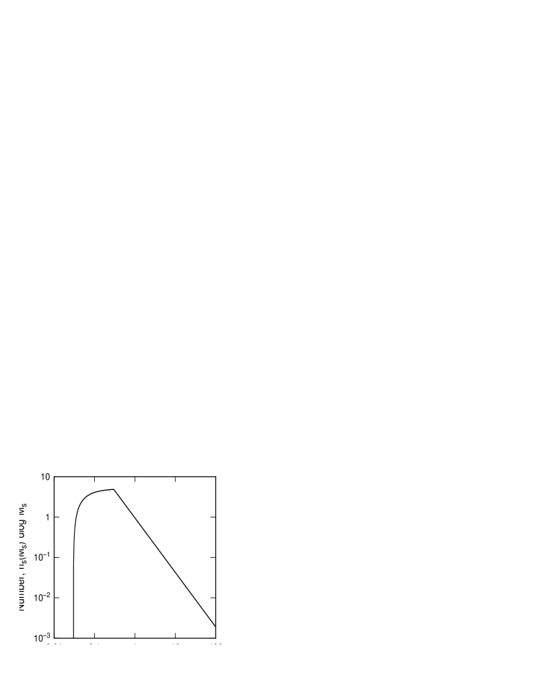
Figure 1: Solution to the analytical expression for the IMF from equations 6 and 7 using ${\cal R}=10$.

Figure 2: IMF model with random sampling from a hierarchical cloud for four values of the mass range ${\cal R}$, defined to be the ratio of the maximum fraction to the minimum fraction of the clump mass that goes into a star. The straight line has a slope of 1.3

Figure 2 shows the result better using the numerical model with random sampling described in Papers I and II, but now with a stellar mass equal to a random fraction $\epsilon$ of the chosen clump mass. This random fraction is equally distributed over a logarithmic range, as specified in the above discussion, by using the equation $\epsilon={\cal R}^{r-1}$ for random variable $r$ that is distributed uniformly over $\left[0,1\right]$. Four different values of ${\cal R}$ are used in the figure to show how the length of the flattened part equals ${\cal R}$. The ${\cal R}=1$ case shows the pure clump selection spectrum, as in papers I and II, but with a sharper lower mass cutoff than in the other papers, taken here from a failure probability $P_{f}=exp\left(-\left[M_{c}/M_{J}\right]^{4}\right)$. We also took $\epsilon_{max,0}=1$ for simplicity; the exact value is not important (it occurs in the expression for $\epsilon(r)$). For all of the cases, there are 10 levels of hierarchical structure in the cloud model, with an average of 2 subpieces per piece, and an actual number of subpieces per piece distributed as a Poisson variable over the interval from 1 to 4.

The results indicate that for $M_{s}>M_{J}\epsilon_{max,0}$, the model IMF is a power law with the same power as the clump mass spectrum obtained previously. The distribution $P\left(\epsilon\right)$ does not affect the IMF above the break point even though it applies there. This is because each chosen clump makes a wide range of stellar masses and contributes a flat component of width ${\cal R}$ to the local IMF, but the sum of the number of stars at each stellar mass is still a power law with the same power as the clump spectrum, independent of $P\left(\epsilon\right)$.

The IMF becomes flat below $M_{J}\epsilon_{max,0}$ because all of the stars there come from clumps with masses near $M_{J}$. In fact, the decreasing nature of the clump spectrum toward higher masses makes clumps with masses very close to $M_{J}$ the favored parents for stars with masses less than $M_{J}\epsilon_{max,0}$. Thus the low mass IMF is determined entirely by the separate mass spectrum for stars that form inside each self-gravitating clump.

Evidently, there are two mass spectra for star formation, one coming from cloud structure and clump selection, giving the Salpeter function, and another coming from star formation inside each clump, giving the flat part. The latter function actually applies everywhere, but it does not visibly affect the Salpeter distribution for intermediate to high masses because stars there have a wide range ($={\cal R}$) of clump masses for parents. It only appears for star masses that form from the lowest mass clumps that can make a star.

The model IMF decreases sharply below the smallest star mass that can form in a clump of mass $M_{J}$, which is $M_{J}\epsilon_{max,0}/{\cal R}$. The parameters $\epsilon_{max,0}$ and ${\cal R}$, as well as the function $P(\epsilon)$, depend on the physics of star formation, unlike $x$ in the power law part of the IMF, which depends primarily on the physics of prestellar cloud structure.

4 Conclusions

The flat part of the IMF is proposed to result from the distribution of the ratio of star mass to clump mass, which must also be flat in logarithmic intervals. Such a distribution shows up only below the mass of the smallest unstable clump mass, so in principle, it might only apply there physically. However, it could apply equally well for all clumps in a star-forming cloud because it does not actually reveal itself at masses above this threshold. The low mass flattening and eventual turnover below the brown dwarf range depend in unspecified ways on the detailed physics of star formation, which also contribute to the single characteristic mass, $M_{J}$. The slope of the power law part of the IMF, above $M_{J}$, depends primarily on cloud structure, although the same complexities of star formation probably apply there too. This is why the Salpeter IMF appears in so many diverse environments: the universal character of turbulent cloud structure determines the power law nature and the power law itself for intermediate to high mass stars, independent of the details of star formation. Variations in the IMF from diverse physical conditions should be much more pronounced at low mass.

This model may be checked observationally by determining the range and distribution function for final star mass in resolved clumps of a given mass. The resolution of the clumps is important so one can be sure the clumps belonging to each individual star or binary pair are measured, and not confused with larger clumps that may include substructure associationed with separate stars. If this model is correct, then the star mass distribution for clumps of a given mass will be much flatter than the Salpeter function, and this may be the case for all clump masses, even those containing intermediate to high mass stars where the Salpeter function applies to the ensemble of stars coming from clumps of different masses.

References

- [1] Comeron, F., Rieke, G.H., Rieke, M.J. 1996, ApJ, 473, 294
- [2] Cool, A.M. 1998, in Gilmore, G., Howell, D., eds., ASP Conf. Ser. Vol. 142, The Stellar Initial Mass Function, Astron. Soc. Pac., San Francisco, p.139
- [3] Elmegreen, B.G. 1993, ApJ, 419, L29
- [4] Elmegreen, B.G. 1997, ApJ, 486, 944
- [5] Elmegreen, B.G. 1999, ApJ, 515, 323
- [6] Elmegreen, B.G., Falgarone, E. 1996, ApJ, 471, 816
- [7] Elmegreen, B.G., Efremov, Yu.N. 2000, in McCaughrean, M.J., Burkert, A., eds., ASP Conf. Ser., The Orion Complex Revisited, in press.
- [8] Festin, L. 1997, A&A, 322, 455
- [9] Fleck, R.C., Jr. 1996, ApJ, 458, 739
- [10] Hillenbrand, L.A. 1997, AJ, 113, 1733
- [11] Hillenbrand, L.A., Carpenter, J. 1999, BAAS 194, 53.01
- [12] Klessen, R.S., Heitsch, F., MacLow, M.-M. 2000, ApJ, in press
- [13] Lada, E.A., Lada, C.J., Muench, A. 1998, in Gilmore, G., Howell, D., eds., ASP Conf. Ser. Vol. 142, The Stellar Initial Mass Function, Astron. Soc. Pac., San Francisco, p.107
- [14] Larson, R.B. 1998, MNRAS, 301, 569
- [15] Luhman, K. L., & Rieke, G. H. 1998, ApJ, 497, 354
- [16] Macintosh, B., Zuckerman, B., Becklin, E.E., & McLean, I.S. 1996, BAAS, 189, 120.05
- [17] Massey, P. 1998, in Gilmore, G., Howell, D., eds., ASP Conf. Ser. Vol. 142, The Stellar Initial Mass Function, Astron. Soc. Pac., San Francisco, p.17
- [18] Miller, G.E., Scalo, J. 1979, ApJS, 41, 513
- [19] Reid, N. 1998, in Gilmore, G., Howell, D., eds., ASP Conf. Ser. Vol. 142, The Stellar Initial Mass Function, Astron. Soc. Pac., San Francisco, p.121
- [20] Rieke, G.H., Lebofsky, M.J., Thompson, R.I., Low, F.J., Tokunaga, A.T. 1980, ApJ, 238, 24
- [21] Salpeter, E.E. 1955, ApJ, 121, 161
- [22] Scalo, J.M. 1985 in Black, D.C., Mathews, M.S., eds., Protostars and Planets II, Univ. of Arizona Press, Tucson, AZ, p.201
- [23] Scalo, J.M. 1998, in Gilmore, G., Howell, D., eds., ASP Conf. Ser. Vol. 142, The Stellar Initial Mass Function, Astron. Soc. Pac., San Francisco, p.201
- [24] Scalo, J.M. 1986, Fund.Cos.Phys, 11, 1
- [25] Stützki, J. 1999, in Ossenkopf, V., Stützki, J., Winnewisser, G., eds. The Physics and Chemistry of the Interstellar Medium, 3rd Cologne-Zermatt Symposium, Shaker-Verlag, Aachen, p. 203