Correlations in the Spatial Power Spectra Inferred from Angular Clustering: Methods and Application to APM

Abstract

We reconsider the inference of spatial power spectra from angular clustering data and show how to include correlations in both the angular correlation function and the spatial power spectrum. Inclusion of the full covariance matrices loosens the constraints on large-scale structure inferred from the APM survey by over a factor of two. We present a new inversion technique based on singular value decomposition that allows one to propagate the covariance matrix on the angular correlation function through to that of the spatial power spectrum and to reconstruct smooth power spectra without underestimating the errors. Within a parameter space of the CDM shape $\Gamma$ and the amplitude $\sigma_{8}$, we find that the angular correlations in the APM survey constrain $\Gamma$ to be 0.19–0.37 at 68% confidence when fit to scales larger than $k=0.2h{\rm\,Mpc}^{-1}$. A downturn in power at $k<0.04h{\rm\,Mpc}^{-1}$ is significant at only 1–$\sigma$. These results are optimistic as we include only Gaussian statistical errors and neglect any boundary effects.

1 Introduction

Even without distance measurements, the large-scale clustering of galaxies can be measured through its projection on the celestial sphere. The angular correlation function and power spectrum provide useful statistics to quantify this clustering; however, in order to compare the results to theoretical models or between different surveys, it is necessary to account for the projection along the line of sight (Limber, 1953; Peebles, 1973; Groth & Peebles, 1977). One approach to this is to deproject the angular statistic to the full spatial power spectrum by assuming the latter to be isotropic in wave number. This inversion, however, requires some form of smoothing, which in turn complicates the propagation of errors. In particular, the correlations of different scales in the angular correlation function and the spatial power spectrum are never negligible and must be handled correctly.

In this paper, we present improvements to two aspects of the deprojection problem. First, we calculate the covariance matrix of the angular correlation function, and the spatial power spectrum derived therefrom, under the approximation of wide sky coverage and Gaussian statistics. The former condition means that we neglect boundary effects; the latter condition means that we neglect contributions from the three- and four-point functions. These are reasonable approximations for the large-angle clustering signal in wide-field sky surveys such as the Automated Plate Measuring (APM) galaxy survey (Maddox et al., 1990), Palomar Digital Sky Survey (DPOSS, Djorgovski et al. 1998), and the Sloan Digital Sky Survey (SDSS). We include both sample variance and shot noise contributions, although the latter is negligible on large angular scales in these surveys. While we cannot estimate the effects of systematic errors, the statistical covariances should provide a lower limit on the uncertainties. We find these limits to be substantially less restrictive than results from earlier analyses.

Second, we present a new, simple inversion technique, based on singular value decomposition (SVD). We use SVD to identify those excursions in the power spectrum that would have minimal effects on the angular clustering observables. We then restrict these directions from having unphysical and numerically intractable effects on the inversion. The errors on the observed angular correlations can be easily propagated to the power spectrum, including the non-trivial correlations between different bins. The best-fit power spectra and covariance matrix converge as the binning in angle and wavenumber is refined.

We then apply both of these improvements to the problem of inferring the spatial power spectrum from the angular clustering of the APM galaxy survey (Maddox et al., 1990). Assuming only Gaussian statistical errors, we reconstruct the binned bandpowers and their covariance matrix. We find large anti-correlated errors. To give a sense of what these results imply for the measurement of the power spectrum on large scales, we fit scale-invariant CDM models to the results at $k<0.2h{\rm\,Mpc}^{-1}$. Varying only the shape parameter $\Gamma$ and the primordial amplitude, we find that $\Gamma$ is constrained to be 0.19–0.37 (68%). Inclusion of non-Gaussianity, survey boundary effects, or systematic errors could make this constraint weaker. While CDM models with $\Gamma\approx 0.25$ are good fits to the data, it is important to note that the statistical power of this fit is dominated by $k>0.1h{\rm\,Mpc}^{-1}$. A turnover in power at $k<0.04h{\rm\,Mpc}^{-1}$ is detected at only 1–$\sigma$. We would therefore not say that the large-angle clustering of APM confirms the shape of the CDM model power spectrum.

One could get tighter limits on $\Gamma$ by extending the fit to smaller scales. On small scales, however, scale-dependent bias and non-linear evolution may minimize and obscure the differences between cosmologies. It is on large scales where the details of the shape of the power spectrum draw unambiguous distinctions between cosmological models. Hence, we have a particular interest in what can be learned at large scales.

Our large-scale constraints are over a factor of two looser than earlier results in the literature. Baugh & Efstathiou (1993, hereafter BE93; 1994) used Lucy inversion to infer the spatial power spectrum from the APM angular correlation function (Maddox et al., 1996). The errors on this power spectrum could only be estimated as the deviation between 4 subsamples of the survey. The small number of subsamples prevented an estimation of the covariance between different wavenumber bins. It is clear that correlations between the subsamples are non-negligible. Moreover, because the smoothing of the power spectra in each subsample was done before the dispersion was computed, the errors are substantially underestimated in poorly constrained regions. Both of these effects lead to overly optimistic constraints. Recently, Dodelson & Gaztañaga (1999, hereafter DG99) presented a different inversion technique based on a Bayesian smoothness prior. Their method allows one to estimate the covariance of the spatial power spectrum from the covariance on the angular correlation function. However, they include only the diagonal elements of the latter covariance matrix. We show that this leads to a factor of two underestimate of the error bars on CDM model parameters. Moreover, like the BE93 method, the DG99 technique systematically underestimates error bars in poorly constrained regions.

The structure of this paper is as follows. In § 2, we present the definitions for clustering statistics and the relations between them. In § 3, we show how to calculate the covariance matrix for the angular correlation function. § 4 describes how to construct the spatial power spectrum using SVD. We then apply these methods to the APM angular clustering in § 5, recovering the correlated bandpowers in § 5.1 and fitting them to CDM models in § 5.2. In § 5.3, we consider the effects of non-Gaussianity and estimate that they are likely to be small. In § 5.4, we demonstrate that the constraints obtained are close to the best-possible errors available to an angular clustering survey with the selection function and sky coverage of APM. We compare our work to previous analyses in § 5.5. We conclude in § 6.

2 Definitions and Relations

Following the usual notation, we take the angular positions of the galaxies to define a continuous fractional overdensity field $\delta({\vec{x}})$, where ${\vec{x}}$ is a position on the sky. We take a flat-sky approximation and define the Fourier modes of this density field as $\delta_{\vec{K}}=\int d^{2}x\delta({\vec{x}})e^{-i{\vec{K}}\cdot{\vec{x}}}$ for all angular wavevectors ${\vec{K}}$. If the random process underlying the density field is translationally-invariant, then ensemble averages of the product of two of these Fourier modes is given by the power spectrum:

$$\left<\delta_{\vec{K}}\delta^{*}_{{\vec{K}}^{\prime}}\right>=(2\pi)^{2}\delta_{D}^{(2)}({\vec{K}}-{\vec{K}}^{\prime})P_{2}({\vec{K}}).$$ (1)

$\delta_{D}^{(2)}$ is the two-dimensional Dirac delta function. The power spectrum $P_{2}$ is the sum of the true power spectrum and a shot noise term equal to the inverse of the number density of sources on the sky. We will assume that $P_{2}$ is isotropic. The angular correlation function is defined as

$$w(\theta)\equiv\left<\delta({\vec{x}})\delta({\vec{x}}+{\vec{\theta}})\right>_{\vec{x}}=\int{d^{2}K\over(2\pi)^{2}}e^{i{\vec{K}}\cdot{\vec{\theta}}}P_{2}(K)=\int{K\,dK\over 2\pi}J_{0}(K\theta)P_{2}(K),$$ (2)

where $J_{0}(x)$ is the Bessel function.

Relating these angular correlations to their parent three-dimensional correlations requires one to include the survey-dependent projection along the line-of-sight. We adopt the Limber approximation to project the spatial clustering (Limber, 1953; Groth & Peebles, 1977; Phillips et al., 1978). This is valid for modes with wavelengths smaller than the survey depth and any evolutionary scale.

The projection is characterized by the redshift distribution $dN/dz$ of the galaxies in the survey. The total number of galaxies per unit solid angle is denoted $N$. The cosmology and the evolution of clustering affect the projection, although for analysis of APM, the differences can be scaled out easily. As we are interested in large scales, we assume that the power spectrum can be separated into a function of redshift $z$ and a function of comoving spatial wavenumber $k$

$$P(k,t)={P(k)\over(1+z)^{a}},$$ (3)

where $P(k)$ denotes the present-day spatial power spectrum (BE93). The function of time is a convolution of the growth of perturbations in the mass, the time evolution of bias, and the effects of luminosity-dependent bias between nearby, faint galaxies and distant, bright ones. Following the notation of BE93, the angular power spectrum is

$$P_{2}(K)={1\over K}\int{dkP(k)f(K/k)}$$ (4)

where the kernel is

$$f(r_{a})=\left[{1\over N}{dN\over dz}{dz\over dr_{a}}\right]^{2}{F(r_{a})\over(1+z)^{a}}.$$ (5)

Here, $r_{a}=K/k$ is the comoving angular diameter distance (or proper motion distance) to a redshift $z$. One has the simple relation

$${dz\over dr_{a}}=E(z)=\left[\Omega_{m}(1+z)^{3}+\Omega_{K}(1+z)^{2}+\Omega_{\Lambda}\right]^{1/2}$$ (6)

where $\Omega_{m}$ is the density in non-relativistic matter, $\Omega_{\Lambda}$ is the cosmological constant, and $\Omega_{K}=1-\Omega_{m}-\Omega_{\Lambda}$. Curvature also enters through the volume correction

$$F(r_{a})=\sqrt{1+(H_{0}r_{a}/c)^{2}\Omega_{K}}.$$ (7)

Combining equations (2) and (4), we can write the angular correlation function as

$$w(\theta) = \int_{0}^{\infty}kP(k)g(k\theta)dk$$ (8)

$$g(k\theta) = {1\over 2\pi}\int dr_{a}J_{0}(k\theta r_{a}){F(r_{a})\over(1+z)^{a}}\left[{1\over N}{dN\over dz}{dz\over dr_{a}}\right]^{2}.$$ (9)

3 Covariance

We are interested in the estimation of the angular correlation function on large angular scales in wide-field surveys. In these surveys, the density of galaxies is large enough that including only shot noise—the sparse sampling of the density field by the galaxies—would severely underestimate the errors. Instead, the errors are dominated by “sample variance”, the uncertainty due to the finite number of patches of the desired angular scale available within the survey. If the angular extent of the survey is large compared to the correlation scales and compared to the angular projection of any clustering scales, then corrections from the boundaries of the survey will be small. In this limit, the effects of sample variance on the angular correlation function can be easily calculated.

Imagine that our survey has a selection window $W({\vec{x}})$ on the sky, with $W=1$ in covered regions and $W=0$ elsewhere. Then the estimator of $w({\vec{\theta}})$ is simply

$$\hat{w}({\vec{\theta}}) = {1\over A({\vec{\theta}})}\int d^{2}xW({\vec{x}})\int d^{2}x^{\prime}W({\vec{x}}^{\prime})\delta({\vec{x}})\delta({\vec{x}}^{\prime})\delta_{D}^{(2)}({\vec{x}}-{\vec{x}}^{\prime}-{\vec{\theta}})$$ (10)

$$= \int{d^{2}K\over(2\pi)^{2}}{d^{2}K_{1}\over(2\pi)^{2}}\delta_{\vec{K}}\delta^{*}_{{\vec{K}}_{1}}e^{i{\vec{K}}_{1}\cdot{\vec{\theta}}}h({\vec{K}}-{\vec{K}}_{1},{\vec{\theta}})$$ (11)

where

$$A({\vec{\theta}})=\int d^{2}xW({\vec{x}})W({\vec{x}}+{\vec{\theta}})$$ (12)

and

$$h({\vec{K}},{\vec{\theta}})={1\over A({\vec{\theta}})}\int d^{2}xe^{i{\vec{K}}\cdot{\vec{\theta}}}W({\vec{x}})W({\vec{x}}+{\vec{\theta}}).$$ (13)

Using Equations (1) and (2), one finds that $\left<\hat{w}({\vec{\theta}})\right>=w({\vec{\theta}})$.

The covariance of this set of estimators can be written

$$C_{w}({\vec{\theta}},{\vec{\theta}}^{\prime}) \equiv \left<[\hat{w}({\vec{\theta}})-w({\vec{\theta}})][\hat{w}({\vec{\theta}}^{\prime})-w({\vec{\theta}})]\right>$$ (14)

$$= \int{d^{2}K\over(2\pi)^{2}}{d^{2}K_{1}\over(2\pi)^{2}}e^{i{\vec{K}}_{1}\cdot{\vec{\theta}}}h({\vec{K}}-{\vec{K}}_{1},{\vec{\theta}})\int{d^{2}K^{\prime}\over(2\pi)^{2}}{d^{2}K^{\prime}_{1}\over(2\pi)^{2}}e^{i{\vec{K}}^{\prime}_{1}\cdot{\vec{\theta}}^{\prime}}h({\vec{K}}^{\prime}-{\vec{K}}^{\prime}_{1},{\vec{\theta}}^{\prime})$$ (16)

$$\times\left[\left<\delta_{\vec{K}}\delta^{*}_{{\vec{K}}_{1}}\delta_{{\vec{K}}^{\prime}}\delta^{*}_{{\vec{K}}^{\prime}_{1}}\right>-\left<\delta_{\vec{K}}\delta^{*}_{{\vec{K}}_{1}}\right>\left<\delta_{{\vec{K}}^{\prime}}\delta^{*}_{{\vec{K}}^{\prime}_{1}}\right>\right].$$

The expectation of four $\delta$’s involves a Gaussian term as well as the four-point function:

$$\begin{array}[]{l}\left<\delta_{\vec{K}}\delta^{*}_{{\vec{K}}_{1}}\delta_{{\vec{K}}^{\prime}}\delta^{*}_{{\vec{K}}^{\prime}_{1}}\right>-\left<\delta_{\vec{K}}\delta^{*}_{{\vec{K}}_{1}}\right>\left<\delta_{{\vec{K}}^{\prime}}\delta^{*}_{{\vec{K}}^{\prime}_{1}}\right>=\\[3.0pt] \hskip 72.26999pt(2\pi)^{2}\delta_{D}^{(2)}({\vec{K}}+{\vec{K}}^{\prime})P_{2}({\vec{K}})(2\pi)^{2}\delta_{D}^{(2)}({\vec{K}}_{1}+{\vec{K}}_{1}^{\prime})P_{2}({\vec{K}}_{1})+\\[3.0pt] \hskip 72.26999pt(2\pi)^{2}\delta_{D}^{(2)}({\vec{K}}-{\vec{K}}_{1}^{\prime})P_{2}({\vec{K}})(2\pi)^{2}\delta_{D}^{(2)}({\vec{K}}_{1}-{\vec{K}}^{\prime})P_{2}({\vec{K}}_{1})+\\[3.0pt] \hskip 72.26999pt(2\pi)^{2}\delta_{D}^{(2)}({\vec{K}}-{\vec{K}}_{1}+{\vec{K}}^{\prime}-{\vec{K}}_{1})T_{4}({\vec{K}},{\vec{K}}_{1},{\vec{K}}^{\prime},{\vec{K}}_{1}^{\prime}).\end{array}$$ (17)

The four-point function $T_{4}$ primarily includes the four-point function of the density, but non-zero shot-noise also introduces terms involving the two- and three-point functions (Hamilton, 1999). We can simplify the Gaussian portion of $C_{w}({\vec{\theta}},{\vec{\theta}}^{\prime})$ to

$$C_{w}({\vec{\theta}},{\vec{\theta}}^{\prime})=\int{d^{2}K\over(2\pi)^{2}}{d^{2}K_{1}\over(2\pi)^{2}}P_{2}({\vec{K}})P_{2}({\vec{K}}_{1})h({\vec{K}}-{\vec{K}}_{1},{\vec{\theta}})h^{*}({\vec{K}}-{\vec{K}}_{1},{\vec{\theta}}^{\prime})\left(e^{i{\vec{K}}_{1}\cdot{\vec{\theta}}+i{\vec{K}}\cdot{\vec{\theta}}^{\prime}}+e^{i{\vec{K}}_{1}\cdot{\vec{\theta}}-i{\vec{K}}_{1}\cdot{\vec{\theta}}^{\prime}}\right).$$ (18)

We will drop the non-Gaussian terms from equation (14). If one assumes Gaussian initial perturbations, then one can use the Gaussian analysis to study large angular and spatial scales. On smaller scales, we expect that non-Gaussianity will contribute considerably more variance due to the correlations between modes (Meiksin et al., 1999a; Scoccimarro et al., 1999). It is important to note that angular clustering statistics tend to have smaller non-Gaussian terms than a simple mapping of the spatial non-linear scale would suggest. This is because one is projecting many non-linear regions along the line-of-sight; the central limit theorem then drives the sum of the fluctuations towards Gaussianity. We note that although this is comforting for the calculation of the angular correlations, it is not clear that the inference of spatial clustering from the angular statistics retains this advantage.

For the particular case of APM, calculations with the hierarchical ansatz (§ 5.3) suggest that non-Gaussian terms become equal to the Gaussian terms at $K\gtrsim 100$, which indicates that our smallest scales are not safely in the Gaussian regime. Unfortunately, the ansatz is not reliable enough to give a useful calculation of the 4-point terms in equation (14) (Scoccimarro et al., 1999). As we will describe in § 5.3, a simple attempt to include non-Gaussianity degraded our results by $\sim$10%. We therefore regard non-Gaussianity as a caveat to our results but not a catastrophic error.

We are interested in the case when the sky coverage of the survey is large, both compared to the angle $\theta$ and to any angular correlation length. Here, the function $h({\vec{K}},{\vec{\theta}})$ becomes sharply peaked around ${\vec{K}}=0$. To leading order, it may be treated as a Dirac delta function. The coefficient is

$$\int{d^{2}K\over(2\pi)^{2}}h({\vec{K}},{\vec{\theta}})h^{*}({\vec{K}},{\vec{\theta}}^{\prime})={\int d^{2}xW^{2}({\vec{x}})W({\vec{x}}+{\vec{\theta}})W({\vec{x}}+{\vec{\theta}}^{\prime})\over A({\vec{\theta}})A({\vec{\theta}}^{\prime})}={1\over A_{\Omega}},$$ (19)

where $A_{\Omega}$ is simply the area of the survey. Effects from boundaries or from features in the power spectrum will be suppressed by another power of $A_{\Omega}$. For wide-angle surveys, we can approximate the correlations in $w(\theta)$ as

$$C_{w}({\vec{\theta}},{\vec{\theta}}^{\prime})={1\over A_{\Omega}}\int{d^{2}K\over(2\pi)^{2}}P_{2}^{2}({\vec{K}})\left[e^{i{\vec{K}}\cdot({\vec{\theta}}+{\vec{\theta}}^{\prime})}+e^{i{\vec{K}}\cdot({\vec{\theta}}-{\vec{\theta}}^{\prime})}\right].$$ (20)

Since we are neglecting all boundary effects, we can average ${\vec{\theta}}$ over angle, i.e. $w(\theta)=(1/2\pi)\int d\phi\,w({\vec{\theta}})$, to yield

$$C_{w}(\theta,\theta^{\prime})\equiv\left<[\hat{w}(\theta)-w(\theta)][\hat{w}(\theta^{\prime})-w(\theta^{\prime})]\right>={1\over\pi A_{\Omega}}\int_{0}^{\infty}dK\,KP_{2}^{2}(K)J_{0}(K\theta)J_{0}(K\theta^{\prime}).$$ (21)

This is the Gaussian contribution to the covariance of the angular correlation function in the limit of a wide-field survey. Our neglect of the boundary terms is equivalent to the approximation that working on a fraction $f_{\rm sky}$ of the sky simply increases the variance on the angular power spectra by $f_{\rm sky}^{-1}$ (Scott et al., 1994).

It is important to note that as the area of a survey increases the covariance in equation 21 does not approach a limit in which errors on different angular scales are statistically independent. This means that analysis of $w(\theta)$ in the sample-variance limit must not neglect the correlation of the error bars on $w(\theta)$. This runs contrary to the properties of $P_{2}$, in which differing scales do become independent in the large-data-set limit of a Gaussian process. We will show later that the inclusion of these correlations substantially weakens the published constraints on the large-scale power spectrum from the APM survey.

Our estimate of $C_{w}$ does not include systematic errors, the effects of non-Gaussian statistics, or aliasing from the survey boundary. It would be very surprising, however, if these complications were to reduce the uncertainty on inferring $P(k)$! In this sense, we consider Equation (21) as a lower bound on the errors.

4 SVD Inversion

We wish to estimate $P(k)$ from observations of $w(\theta)$. In practice, we are given estimates of $w$ in $N_{\theta}$ bins centered on angles $\theta_{j}$ ($j=1,\ldots,N_{\theta}$). We denote the estimates as $w_{j}$ and place them in a vector ${\mathbf{w}}$. These measurements have a $N_{\theta}\times N_{\theta}$ covariance matrix $C_{w}$.

We then wish to estimate $P(k)$ in $N_{k}$ bins centered at $k_{j}$ ($j=1,\ldots,N_{k}$). The values in these bins are denoted $P_{j}$ and formed into a vector ${\mathbf{P}}$. The integral transform of equation (8) can then be cast as a matrix, yielding

$${\mathbf{w}}=G{\mathbf{P}},$$ (22)

where $G$ is a $N_{\theta}\times N_{k}$ matrix.

In detail, one should calculate the elements of $G$ taking account of the averaging in the bins of $k$ and $\theta$. The method of averaging can be chosen, but if one takes the estimates $w_{j}$ to be averages of $w(\theta)$ according to the weight $\theta d\theta$ and treats $P(k)$ as constant within a bin in $k$, then the integrals over $k$ and $\theta$ can be done analytically using properties of the Bessel function. We find, however, that for reasonably narrow bins the approximate treatment of using only the central values of $\theta$ and $k$ produces nearly the same answer as the exact integration.

With this notation, the best-fit power spectrum is simply $\hat{\bf P}=G^{-1}{\mathbf{w}}$ and the covariance matrix on this inversion is $C_{P}^{-1}=G^{T}C_{w}^{-1}G$. It is important to note that this covariance matrix is not diagonal, even in the large survey volume limit. This differs from the behavior of estimates of $P_{3}(k)$ from a redshift survey, where individual bins approach independence in the large-volume limit.

In practice, the matrix $G$ is nearly singular, as one would guess from its origin as a projection from 3 dimensions to 2. By singular, we mean that the matrix has a non-zero null space, i.e. that there are vectors ${\mathbf{P}}$ that are annihilated by $G$. Such null directions cannot be constrained from the angular data. Often the near singularities come about from having too fine a binning in $k$ or from extending the domain in $k$ to values that have negligible impact on the range of angular scales being measured. Left untreated, these directions introduce wild excursions in $P(k)$ in order to compensate tiny variations in $w(\theta)$. The resulting covariance matrix $C_{P}$ has enormous, but highly anti-correlated, errors.

Singular value decomposition offers a useful way to treat this singularity. If we take the measurements ${\mathbf{w}}$ to be Gaussian-distributed around their true values ${\mathbf{w}}_{m}$, then the distribution of the observations follows the probability $P\propto\exp(-\chi^{2}/2)$, where

$$\chi^{2}=({\mathbf{w}}_{m}-{\mathbf{w}})^{T}C_{w}^{-1}({\mathbf{w}}_{m}-{\mathbf{w}}).$$ (23)

${\mathbf{w}}_{m}$ is related to the true power spectrum by ${\mathbf{w}}_{m}=G{\mathbf{P}}_{m}$. We will rescale the basis set for ${\mathbf{P}}_{m}$ by dividing by a set of reference values ${\mathbf{P}_{\rm norm}}$, intended to be defined by a fiducial power spectrum $P_{\rm norm}(k)$ evaluated at the appropriate wavenumbers. This produces ${\mathbf{P}}^{\prime}$ by dividing each element of ${\mathbf{P}}$ by the corresponding element of ${\mathbf{P}_{\rm norm}}$. We also define ${\mathbf{w}}^{\prime}=C_{w}^{-1/2}{\mathbf{w}}$ and $G^{\prime}=C_{w}^{-1/2}G{\mathbf{P}_{\rm norm}}$; here, $C_{w}^{-1/2}$ is constructed by taking the inverse square root of the eigenvalues of the positive-definite $C_{w}$ matrix. We then have

$$\chi^{2}=|G^{\prime}{\mathbf{P}}^{\prime}_{m}-{\mathbf{w}}^{\prime}|^{2}.$$ (24)

Finding the vector (or subspace) ${\mathbf{P}}^{\prime}_{m}$ that minimizes $\chi^{2}$, and thereby maximizes the likelihood in a Gaussian treatment, is a prime application of SVD, and the technique allows one to treat the nearly singular directions in $P$-space explicitly. Note that we can immediately see that the covariance matrix of the ${\mathbf{P}}^{\prime}_{m}$ will simply be $(G^{\prime T}G^{\prime})^{-1}$. We will now drop the $m$ subscript and refer to the reconstructed power spectrum as ${\mathbf{P}}^{\prime}$.

We define the SVD of the $G^{\prime}$ matrix by $G^{\prime}=UWV^{T}$ (Press et al., 1992, for a review), where $W$ is a square, diagonal matrix of the singular values (SV), $V$ is a $N_{k}\times N_{k}$ orthogonal matrix, and $U$ is a $N_{\theta}\times N_{k}$ column-orthonormal matrix. Singular values close to zero correspond to columns in $V$ that contain ${\mathbf{P}}^{\prime}$ directions that have almost no effect on ${\mathbf{w}}^{\prime}$ and therefore are not well-constrained. To find the best-fit power spectrum, we use ${\mathbf{P}}^{\prime}=VW^{-1}U^{T}{\mathbf{w}}^{\prime}$. The covariance matrix $C_{P}$ of ${\mathbf{P}}^{\prime}$ is simply $VW^{-2}V^{T}$, which is the diagonalization of the covariance matrix.

Mathematically, the fact that the $W$ matrix is diagonal means that the data ${\mathbf{w}}^{\prime}$ is coupled to the power spectrum estimate ${\mathbf{P}}^{\prime}$ through $N_{k}$ distinct modes, in which the matching columns of the $U$ and $V$ matrix specify a matching set of ${\mathbf{w}}^{\prime}$ and ${\mathbf{P}}^{\prime}$ excursions. We denote the $j$th SV as $W_{j}$ and the $j$th column of $U$ and $V$ as $U_{j}$ and $V_{j}$, respectively. We refer to the set $W_{j}$, $U_{j}$, and $V_{j}$ as the $j$th SV mode. In detail, each mode enters the best-fit power spectrum as $P_{i}=P_{{\rm norm},i}V_{ji}W_{j}^{-1}U_{j}^{T}{\mathbf{w}}^{\prime}$. Comparing this to the formula for $C_{P}$ shows that $U_{j}^{T}{\mathbf{w}}^{\prime}$ is the number of standard deviations by which the $j$th mode is demanded by ${\mathbf{w}}^{\prime}$. Indeed, $\chi^{2}$ may be rewritten as

$$\chi^{2}=|{\mathbf{w}}^{\prime}|^{2}-\sum_{j}|U_{j}^{T}{\mathbf{w}}^{\prime}|^{2},$$ (25)

so the value of $(U_{j}^{T}{\mathbf{w}}^{\prime})^{2}$ is the amount by which the inclusion of a mode in ${\mathbf{P}}^{\prime}$ will decrease $\chi^{2}$. Since the columns of $V$ are unit-normalized, the quantity $W_{j}^{-1}U_{j}^{T}{\mathbf{w}}^{\prime}$ is a measure of the size of the contribution that this mode makes to the power spectrum in units of ${\mathbf{P}_{\rm norm}}$.

Of course, such an analysis is only useful if it converges as the binning of $k$ and $\theta$ becomes finer. In our APM example (§ 5), we find that this is the case: the columns in $U$ and $V$ corresponding to large singular values change very little as we alter the binning in $k$ or $\theta$. The large $W_{j}$ scale as $N_{k}^{-1/2}$ because if one simply refines the binning in $k$, the elements of $G$ scale as $N_{k}^{-1}$ due to the smaller range $dk$ in the defining integral while the elements of $V_{j}$ scale as $N_{k}^{-1/2}$ because it is an unit-normalized vector. The primary effect of adding or removing bins is to change the number of tiny singular values. The modes with large SV show broad tilts and curves in $P(k)$; the modes with small SV show rapid compensating oscillations as well as excursions at very large or small $k$ that the $w(\theta)$ data don’t constrain. The ability to identify the excursions in $P(k)$-space that are well-constrained, in a manner that converges as the binning becomes finer, is the strength of the SVD method. It should be noted that the kernel and its SVD decomposition depend on the survey geometry, the $C_{w}$ covariance matrix, and the fiducial scaling ${\mathbf{P}_{\rm norm}}$, but not upon the observed data ${\mathbf{w}}$ itself.

Left untreated, the small singular values will have large inverses and therefore produce large excursions in ${\mathbf{P}}^{\prime}$. Such excursions are unphysical and can even make $C_{P}$ numerically intractable. In the usual spirit of SVD, we wish to adjust the treatment of these singular values. This is complicated by the fact that SVD relies upon the concepts of orthogonality and normalization and thereby implies a geometric structure that our $P$- and $w$-spaces don’t actually have. To sort the singular values and declare some of them to be “small” requires that we have some sense of comparing $w$ at different values of $\theta$ or $P$ at different values of $k$. On the ${\mathbf{w}}^{\prime}$-space side, this choice is easy: the absorption of $C_{w}$ into $G^{\prime}$ and $w^{\prime}$ means that the unit-normalization of fluctuations in ${\mathbf{w}}^{\prime}$ have the correct role in the $\chi^{2}$ statistic. However, for ${\mathbf{P}}^{\prime}$-space, the choice is more arbitrary. The fiducial power spectrum ${\mathbf{P}_{\rm norm}}$ determines how fluctuations in power on different scales but of equal statistical significance are to be weighted in the singular values. By choosing ${\mathbf{P}_{\rm norm}}$ to be close to the observed spectrum, we are opting that equal fractional excursions on different scales receive equal weight. Had we instead chosen ${\mathbf{P}_{\rm norm}}$ to be a constant, a 100% oscillation at the peak of the power spectrum ($P\approx 10^{4}h^{-3}{\rm\,Mpc^{3}}$ at $k\approx 0.05h{\rm\,Mpc}^{-1}$) would have been suppressed relative to the same fractional fluctuation at smaller scales (say, $P\approx 10^{2}h^{-3}{\rm\,Mpc^{3}}$ at $k\approx 1h{\rm\,Mpc}^{-1}$). It is important to remember that ${\mathbf{P}_{\rm norm}}$ is irrelevant if one is using all of the singular values unmodified. It enters only when we place a threshold on the singular values (as described below). When small singular values are altered or eliminated, ${\mathbf{P}_{\rm norm}}$ determines how different scales are to be compared in the application of a smoothness condition. While the arbitrary choice of ${\mathbf{P}_{\rm norm}}$ means that an SVD treatment of the inversion is not unique, we feel that our ${\mathbf{P}_{\rm norm}}$ is a well-motivated choice: each singular value represents the square root of the $\chi^{2}$ contribution for a given fractional excursion around the best-fit power spectrum.

We next describe how we alter the small $W_{j}$. In detail, we incorporate two different SV thresholds, one for the construction of $C_{P}$ and another for the construction of ${\mathbf{P}}^{\prime}$. Small SV indicate poorly constrained directions. We would like $C_{P}$ to reflect this, but not to the extent that the matrix becomes numerically intractable. Physically, these small $W_{j}$ are highly oscillatory, and our prior from both theory and previous observations is that enormous (much greater than unity) fluctuations don’t exist in the power spectrum. Hence, when constructing $C_{P}$, we increase all SV to a minimum level of $SV_{C}$. We can’t recommend a choice of $SV_{C}$ for arbitrary applications because all the $W_{j}$ will scale with the normalization of ${\mathbf{P}_{\rm norm}}$. However, in our work, where ${\mathbf{P}_{\rm norm}}$ has a similar amplitude to the actual power spectrum, a choice of $SV_{C}$ between 0.1 and 1.0 will allow order unity fluctuations in the power spectrum. This is larger than any oscillations ever seen but not so large as to make $C_{P}$ overly singular.

Without correcting the small $W_{j}$, the best-fit power spectrum ${\mathbf{P}}^{\prime}$ becomes wildly fluctuating. If we have modified the small $W_{j}$ in $C_{P}$, then these fluctuations will appear to be highly significant. Hence, at a minimum one must use the same $W_{j}$ in ${\mathbf{P}}^{\prime}$ as those used in $C_{P}$, so as to keep the fluctuations and the covariance on the same scale. However, since the small SV modes have already been granted an error budget larger than what is likely observable, there is no reason to include them in the best-fit ${\mathbf{P}}^{\prime}$ at all. The difference between the best-fit power spectrum and any reasonably smooth model power spectrum will be insignificant with respect to the covariance $C_{P}$. Hence, we generally only include in ${\mathbf{P}}^{\prime}$ the modes with the largest SV. Essentially this is a threshold on $W_{j}$ for inclusion in the nominal best-fit. In practice, when comparing between spectra calculated with different $C_{w}$ (as we will occasionally do in next section), it is better to keep a fixed number of SV modes rather than fixed $W_{j}$ threshold because the $W_{j}$ will change even while the SV spectrum and the structure of the $U$ and $V$ matrices remains fairly constant.

The modification of $W^{-1}$ when calculating ${\mathbf{P}}^{\prime}$ causes ${\mathbf{P}}^{\prime}$ to be a biased estimator of the power spectrum. This bias is statistically significant at a level of $(1-W_{j}/W_{j,\rm used})\left|U_{j}^{T}{\mathbf{w}}^{\prime}\right|$, where $W_{j,\rm used}$ is the value of $W_{j}$ actually used in constructing ${\mathbf{P}}^{\prime}$ ($\infty$ if the mode has been dropped). One can thereby judge the statistically significance of the bias imposed by altering a $W_{j}$ and decide whether an excursion of the amplitude implied by the original $W_{j}$ is physically reasonable. Of course, one only wishes to drop modes that are statistically irrelevant or physically unreasonable. It is important to remember that the small $W_{j}$ can be strongly perturbed by small changes in $C_{w}$. Since one cannot hope to control all systematic errors in $C_{w}$, one doesn’t want to place any weight on the SV modes with small $W_{j}$.

The bias from increasing $W_{j}$ or omitting modes in ${\mathbf{P}}^{\prime}$ pulls the amplitude of the altered modes toward zero. Usually this pulls the power toward zero, but we can alter this behavior by subtracting $GP_{\rm bias}$ from the $w(\theta)$ data and adding $P_{\rm bias}$ to the reconstructed power spectrum. In other words, one alters equation (24) to

$$\chi^{2}=|G^{\prime}({\mathbf{P}}^{\prime}_{m}-P_{\rm bias})-({\mathbf{w}}^{\prime}-G^{\prime}P_{\rm bias})|^{2},$$ (26)

and reconstructs ${\mathbf{P}}^{\prime}_{m}-P_{\rm bias}$. The bias then pulls toward $P_{\rm bias}$.

All of the above techniques apply equally well to the problem of inferring the spatial power spectrum from the angular power spectrum, and it is trivial to alter the equations.

5 APM

5.1 Reconstructing the Power Spectrum

One of the most influential uses of angular clustering in the last decade has been its application to the APM survey (Maddox et al., 1990). However, a full treatment of the covariance matrix on power spectra inferred from APM clustering has not yet been presented, and so we choose this as our example. We take the data on the APM angular correlation function (Maddox et al., 1996) as presented in the binned results of DG99. This includes 40 half-degree bins from $0^{\circ}.5$ to $20^{\circ}$. Tests show that including data from smaller angular scales does not affect our results on scales larger than $k=0.2h{\rm\,Mpc}^{-1}$.

We discard the quoted errors on the DG99 $w(\theta)$ data and instead use the covariance matrix from § 3. For $P_{2}$, we use

$$P_{2}(K)=\left\{\begin{array}[]{ll}2\times 10^{-4}&K<20\\ 2\times 10^{-4}(K/20)^{-1.35}&K>20,\end{array}\right.$$ (27)

which is a reasonable fit to the results of Baugh & Efstathiou (1994). We assume a survey area of 1.31 steradians. We add a shot noise term of $P_{\rm shot}=1/\bar{n}=10^{-6}$, based on a number density $\bar{n}$ of 1 galaxy per $3^{\prime}.5$ square pixel (Baugh & Efstathiou, 1994). The shot noise has little impact on the results. We use this $P_{2}$ to calculate $C_{w}$ according to equation (21).

We assume $\Omega_{m}=1$, $\Omega_{\Lambda}=0$, and $a=0$ in the calculation. The results do depend on these choices, but nearly all of the behavior can be scaled out in two easy parts. First, the fact that the average galaxy in the survey is at $z\approx 0.11$ means that specifying a time evolution of the power spectrum ($a\neq 0$) will cause a shift in the amplitude of the $z=0$ power spectrum. In practice, one can consider the reconstructed power spectrum to be appropriate to $z=0.11$; in other words, choosing different time dependences for the power spectrum leaves the power at $z=0.11$ essentially constant. Second, the cosmology enters through the volume available at higher redshift. Models with more volume per unit redshift (lower $dz/dr_{a}$) have more modes and therefore suffer more dilution in angular clustering when projected. This effect scales roughly as $E(z=0.11)^{-2}$. Despite the low median redshift, this is not a small effect in $\Lambda$ models: using an $\Omega_{m}=0.3$, $\Omega_{\Lambda}=0.7$ model yields a $P_{3}(k)$ 20% higher than our fiducial model. The effect is much smaller in open models. In detail, $a\neq 0$ or a change in the cosmology will also shift the average depth of the survey slightly, causing the reconstructed power spectrum to move in wavenumber. We find this effect to be less than 5%, which is certainly within the errors.

We use a logarithmic binning in $k$-space. Our fiducial set uses 3 bins per octave, ranging from $k=0.0125h{\rm\,Mpc}^{-1}$ to $k=0.8h{\rm\,Mpc}^{-1}$. There is also a large-scale bin of $k<0.0125h{\rm\,Mpc}^{-1}$, for a total of 19 bins. Wavenumbers greater than $0.8h{\rm\,Mpc}^{-1}$ are not constrained by data at $\theta>0^{\circ}.5$ and would simply be degenerate with our last bin. We also tried coarser and finer binnings, using 2 and 4 bins per octave to get 13 and 25 bins, respectively. These three choices are shown in Table 1 under the names $k13$, $k19$, and $k25$. We find equivalent results with non-logarithmic binning schemes.

We set ${\mathbf{P}_{\rm norm}}$ to be

$$P_{\rm norm}(k)={1.5\times 10^{4}h^{-3}Mpc^{3}\over\left[1+(k/0.05hMpc^{-1})^{2}\right]^{0.65}}$$ (28)

This is a rough fit to the observed power spectrum until $k\approx 0.05h{\rm\,Mpc}^{-1}$ and has constant power on the largest scales. Recall that ${\mathbf{P}_{\rm norm}}$ enters only in the treatment of small singular values and serves to set an upper bound on the allowed size of fluctuations in the power spectrum relative to the best-fit. The constant power on large scales was chosen so as not to prejudice the results on scales where we have little information. It is important to choose $P_{\rm norm}$ to be continuous because the prior against rapid oscillations acts on the ratio of the fitted power spectrum to ${\mathbf{P}_{\rm norm}}$. Discontinuities in $P_{\rm norm}$ would impose discontinuities in the fitted power spectrum.

Table 1:

Singular Values and $k$-space Bins
$k$ bins ($h{\rm\,Mpc}^{-1}$) Singular Values, scaled to 19 bins k13 k19 k25 $W_{k13}\times\left({13\over 19}\right)^{1/2}$ $W_{k19}$ $W_{k25}\times\left({25\over 19}\right)^{1/2}$ 0.000–0.0125 0.000–0.0125 0.000–0.0125 17.1 17.1 17.1 0.0125–0.018 0.0125–0.016 0.0125–0.015 9.2 9.3 9.3 0.018–0.025 0.016–0.020 0.015–0.018 5.2 5.3 5.3 0.025–0.035 0.020–0.025 0.018–0.021 3.1 3.2 3.2 0.035–0.050 0.025–0.032 0.021–0.025 2.0 2.0 2.1 0.050–0.071 0.031–0.040 0.025–0.030 1.4 1.5 1.5 0.071–0.100 0.040–0.050 0.030–0.035 1.0 1.1 1.2 0.100–0.141 0.050–0.063 0.035–0.042 0.80 0.88 0.93 0.141–0.200 0.063–0.079 0.042–0.050 0.53 0.59 0.62 0.200–0.283 0.079–0.100 0.050–0.059 0.30 0.37 0.39 0.283–0.400 0.100–0.126 0.059–0.071 0.12 0.22 0.23 0.400–0.566 0.126–0.159 0.071–0.084 0.014 0.12 0.13 0.566–0.800 0.159–0.200 0.084–0.100 $2.9\times 10^{-4}$ 0.066 0.073 0.200–0.252 0.100–0.119 0.038 0.040 0.252–0.317 0.119–0.141 0.018 0.020 0.317–0.400 0.141–0.168 $3.8\times 10^{-3}$ $9.6\times 10^{-3}$ 0.400–0.504 0.168–0.200 $1.9\times 10^{-4}$ $4.1\times 10^{-3}$ 0.504–0.635 0.200–0.238 $3.3\times 10^{-6}$ $1.7\times 10^{-3}$ 0.635–0.800 0.238–0.283 $3.7\times 10^{-8}$ $6.6\times 10^{-4}$ 0.283–0.336 $3.0\times 10^{-4}$ 0.336–0.400 $2.0\times 10^{-5}$ 0.400–0.476 $1.3\times 10^{-6}$ 0.476–0.566 $1.5\times 10^{-7}$ 0.566–0.673 $2.7\times 10^{-8}$ 0.673–0.800 $4.2\times 10^{-9}$

NOTES.—We scale the $W_{j}$ by $(N_{k}/19)^{1/2}$ to remove the predicted scaling that occurs when one refines the binning in wave number.

Figure 1: Selected pairs of columns from the $U$ and $V$ matrices. The $U$ column indicates the overlap with the ${\mathbf{w}}^{\prime}\equiv C_{w}^{-1/2}{\mathbf{w}}$ data, while the $V$ column indicates the impact on ${\mathbf{P}}$ (as normalized by ${\mathbf{P}_{\rm norm}}$). The singular value of each pair is also given. The noise in the last $U$ vector is the result of the linear binning in $\theta$.

With $C_{w}$ and ${\mathbf{P}_{\rm norm}}$, we can construct the kernel $G^{\prime}$ and find its singular value decomposition. Table 1 shows the spectrum of singular values for each of these 3 choices of binning. When one corrects by $N_{k}^{1/2}$ to account for the default scaling in $W_{j}$, the large singular values are very stable as the binning is refined. Increasing the number of bins only increases the number of very small singular values. This demonstrates that 19 bins is a fine enough grid to characterize the power spectrum; increasing to 25 bins would only add degrees of freedom that are unconstrained by the angular data. We could have put the factor of $N_{k}^{1/2}$ into the definition of ${\mathbf{P}_{\rm norm}}$ so as to make the large $W_{j}$ stable against changes in binning, but since we will hereafter work only with $N_{k}=19$, we opted against the extra complication.

Table 2:

Overlap of Singular Values with APM Data
$W_{j}$ $U_{j}^{T}{\mathbf{w}}^{\prime}$ $W_{j}^{-1}U_{j}^{T}{\mathbf{w}}^{\prime}$ $W_{j,\rm eff}^{-1}U_{j}^{T}{\mathbf{w}}^{\prime}$ 17.1 21.2 1.2 1.2 9.3 7.8 0.84 0.84 5.3 9.0 1.7 1.7 3.2 4.4 1.4 1.4 2.0 -4.1 -2.0 -2.0 1.5 2.3 1.6 1.6 1.1 -1.1 -1.0 -1.0 0.88 -0.56 -0.64 -0.64 0.59 -1.5 -2.6 -2.6 0.37 -0.79 -2.1 -1.6 0.22 -0.96 -4.4 -1.9 0.12 -1.5 -12.4 -3.1 0.066 -0.30 -4.5 -0.60 0.038 -0.56 -14.9 -1.1 0.018 0.082 4.5 0.16 $3.8\times 10^{-3}$ 1.2 $3.3\times 10^{2}$ 2.5 $1.9\times 10^{-4}$ -0.31 $-1.6\times 10^{3}$ -0.61 $3.3\times 10^{-6}$ 0.36 $1.1\times 10^{5}$ 0.72 $3.7\times 10^{-8}$ -1.6 $-4.2\times 10^{7}$ -3.1

NOTES.—The singular values are listed as $W_{j}$. $U_{j}^{T}{\mathbf{w}}^{\prime}$ shows the dot product between the $j$th column of the $U$ matrix and the data vector ${\mathbf{w}}^{\prime}$. $W_{j,\rm eff}$ is the value of the $j$th SV rounded up to a minimum value of $SV_{C}=0.5$.

As described in § 4, the matching columns $U_{j}$ and $V_{j}$ map fluctuations in ${\mathbf{w}}^{\prime}$ to those in ${\mathbf{P}}^{\prime}$ with an amplitude equal to the inverse of the singular value $W$. Figure 1 displays 5 pairs of columns from the SVD. One sees that the large $W_{j}$ are associated with small angular scales in ${\mathbf{w}}^{\prime}$ and with smooth, large $k$ excursions in ${\mathbf{P}}^{\prime}$. As the $W_{j}$ decrease, the oscillations become wilder and move to larger angular scales. The $U_{j}$ and $V_{j}$ vectors for large $W_{j}$ remain very similar as one changes from $k19$ to $k25$ binning.

In Table 2, we look at the overlap of these SV modes with the APM ${\mathbf{w}}^{\prime}$. The quantity $U_{j}^{T}{\mathbf{w}}^{\prime}$ is the number of standard deviations by which the $j$th mode is demanded by ${\mathbf{w}}^{\prime}$. Dividing that by $W_{j}$ yields the amplitude of the effect on the power spectrum (in units of ${\mathbf{P}_{\rm norm}}$). Modes with $U_{j}^{T}{\mathbf{w}}^{\prime}\lesssim 1$ are not statistically significant, while modes with $W_{j}^{-1}U_{j}^{T}{\mathbf{w}}^{\prime}\gg 1$ put enormous fluctuations in the power spectrum that are probably unphysical. One sees that the first 6 modes are clearly demanded, while the remainder are of marginal significance. We will include 8 modes in our quoted results, because this seems to be the transition between smooth and an oscillatory reconstruction. However, we will also perform fits to CDM models with all modes included in ${\mathbf{P}}^{\prime}$. In this regard, we also quote $W_{j,\rm eff}^{-1}U_{j}^{T}{\mathbf{w}}^{\prime}$ in Table 2, where $W_{j,\rm eff}$ is $W_{j}$ rounded up to $SV_{C}=0.5$. This is to remind the reader that the value of $W_{j}$ used in $C_{P}$ is the one used in ${\mathbf{P}}^{\prime}$.

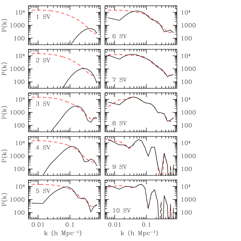
Figure 2: The evolution of $P(k)$ as we include smaller singular values. (solid) The results with $P_{\rm bias}=0$. (dashed) The results with $P_{\rm bias}=P_{\rm norm}$. The fact these two are identical with 8 SV shows that the resulting power spectrum is not being biased by the SVD reconstruction.

In Figure 2, we show how the reconstructed power spectrum develops as we add more SV modes. The largest $W_{j}$ contribute mostly small-scale power. With 6 or 8 modes, a fairly smooth shape appears that matches the expected form of $P(k)$. Adding smaller modes quickly makes the spectrum more oscillating, even with the artificial increase in the $W_{j}$. As Table 2 shows, these oscillations are not statistically significant.

Figure 2 also shows the reconstructed power spectrum if one chooses $P_{\rm bias}=P_{\rm norm}$. Recall that $P_{\rm norm}$ was chosen to have a large amount of power on large scales. This means that any bias in ${\mathbf{P}}^{\prime}$ due to the alteration of SV will pull the spectrum toward high $P$ rather than $P=0$. This allows us to determine how many SV must be included to avoid bias in the large-scale power spectrum. One sees that with 8 modes, the two power spectra are indistinguishable at $k>0.02h{\rm\,Mpc}^{-1}$. This demonstrates that the smooth portion of the power spectrum is being reconstructed in an unbiased way by the SVD method. In different words, the first 8 modes are all that is needed to describe a smooth power spectrum like $P_{\rm norm}$. Note that this does not mean that features in the resulting power spectrum are statistically significant; that depends on the covariance matrix $C_{P}$.

Table 3:

Reconstructed APM Power Spectrum
$k$ Range $P(k)$ $(C_{P})_{jj}^{1/2}$ $(C_{P}^{-1})_{jj}^{-1/2}$ 0.0000–0.0125 6088 22557 18091 0.012–0.016 3802 27469 24706 0.016–0.020 6127 26254 22338 0.020–0.025 9354 24806 19804 0.025–0.032 12891 22724 16836 0.031–0.040 15175 19909 13607 0.040–0.050 14625 17426 10874 0.050–0.063 11458 14855 8324 0.063–0.079 7724 11813 5643 0.079–0.100 5544 9155 3474 0.100–0.126 5077 6948 2061 0.126–0.159 4331 5151 1210 0.159–0.200 2394 3827 710 0.200–0.252 978 2731 417 0.252–0.317 936 2053 247 0.317–0.400 776 1438 147 0.400–0.504 206 1055 90.6 0.504–0.635 252 855 61.0 0.635–0.800 401 422 55.2

NOTES.—This is the best-fit power spectrum using 8 SV to construct ${\mathbf{P}}^{\prime}$ and $SV_{C}=0.5$ in $C_{w}$. The fit to the observed $P_{2}$ (eq. 27) was used to calculate $C_{w}$. The units on wavenumber are $h{\rm\,Mpc}^{-1}$ and on power are $h^{-3}{\rm\,Mpc^{3}}$. Also shown are the diagonal elements of $C_{P}$ and $C_{P}^{-1}$, converted to give a standard deviation on $P(k)$. These are not very useful without the correlations in Table 4. However, they do give the uncertainty on a single $k$ bin when marginalizing and not marginalizing, respectively, over all others. In detail, this is the power at $z=0.11$ in an $\Omega_{m}=1$ cosmology. The power spectrum (and errors) would increase by about $20\%$ in a $\Lambda=0.7$ cosmology due to extra dilution of the angular clustering caused by the additional volume at higher $z$. The corrections in an open cosmology are $\sim\!3\%$.

Table 4:

Reduced Covariance Matrix and Inverse Covariance Matrix for $P(k)$
1.00 -0.24 -0.27 -0.25 -0.15 0 0.10 0.08 0.01 -0.05 -0.02 0.03 0.01 -0.02 0 0.01 -0.01 0 0.01 1.00 -0.10 -0.09 -0.07 -0.03 0.01 0.02 0.01 -0.01 -0.01 0 0 0 0 0 0 0 0 1.00 1.00 -0.13 -0.11 -0.07 -0.02 0.01 0.02 0 -0.01 0 0.01 0 0 0 0 0 0 0.39 1.00 1.00 -0.16 -0.14 -0.08 -0.02 0.03 0.02 -0.01 -0.02 0.01 0.01 -0.01 0 0 -0.01 0 0.44 0.29 1.00 1.00 -0.24 -0.19 -0.08 0.03 0.06 0 -0.03 0.01 0.02 -0.01 0 0.01 0 0 0.43 0.30 0.38 1.00 1.00 -0.32 -0.19 -0.02 0.07 0.03 -0.04 -0.01 0.03 0 -0.02 0.01 0.01 -0.01 0.33 0.26 0.35 0.46 1.00 1.00 -0.32 -0.16 0.01 0.07 0 -0.04 0.01 0.02 -0.02 0 0.02 -0.02 0.18 0.17 0.27 0.41 0.56 1.00 1.00 -0.37 -0.16 0.06 0.08 -0.04 -0.03 0.03 0 -0.02 0.01 -0.01 0.05 0.09 0.18 0.33 0.50 0.65 1.00 1.00 -0.45 -0.13 0.11 0.06 -0.07 -0.02 0.05 -0.01 -0.03 0.04 -0.01 0.04 0.10 0.21 0.36 0.53 0.68 1.00 1.00 -0.51 -0.08 0.16 0.01 -0.08 0.05 0.02 -0.04 0.04 -0.02 0.01 0.04 0.09 0.19 0.32 0.50 0.72 1.00 1.00 -0.56 -0.04 0.17 -0.02 -0.08 0.04 0.03 -0.05 -0.01 0 0.01 0.03 0.07 0.14 0.29 0.53 0.79 1.00 1.00 -0.62 0.04 0.18 -0.11 -0.03 0.08 -0.08 0 0 0 0.01 0.02 0.05 0.12 0.30 0.57 0.83 1.00 1.00 -0.65 0.06 0.18 -0.08 -0.06 0.11 0 0 0 0 0.01 0.02 0.04 0.13 0.32 0.60 0.86 1.00 1.00 -0.68 0.20 0.11 -0.14 0.11 0 0 0 0 0 0.01 0.02 0.05 0.15 0.34 0.61 0.87 1.00 1.00 -0.76 0.17 0.19 -0.27 0 0 0 0 0 0 0.01 0.02 0.06 0.15 0.34 0.61 0.88 1.00 1.00 -0.66 0.17 0.04 0 0 0 0 0 0 0 0.01 0.02 0.06 0.16 0.34 0.61 0.88 1.00 1.00 -0.81 0.62 0 0 0 0 0 0 0 0 0.01 0.02 0.07 0.16 0.34 0.62 0.88 1.00 1.00 -0.95 0 0 0 0 0 0 0 0 0 0.01 0.02 0.07 0.16 0.35 0.62 0.89 1.00 1.00 0 0 0 0 0 0 0 0 0 0 0 0.02 0.06 0.17 0.36 0.64 0.90 1.00 0 0 0 0 0 0 0 0 0 -0.01 -0.01 -0.01 0.01 0.05 0.17 0.41 0.72 0.94 1.00

NOTES.—The upper triangle shows $C_{P}$ after we have divided each row and column by the square root of its respective diagonal element. The lower triangle shows $C_{P}^{-1}$ with its diagonal divided out. Both matrices are symmetric of course. The square root of the diagonal of $C_{P}$ is given as the third column of Table 3; the inverse of the square root of the diagonal of $C_{P}^{-1}$ is the last column in that chart. Please note that well-constrained directions have small eigenvalues in $C_{P}$ and large eigenvalues in $C_{P}^{-1}$. With only two significant figures, the small eigenvalues will be inaccurate. $C_{P}$ is quoted here only to show the correlation coefficients. If one wishes to fit smooth power spectrum models using the above matrices, one must use $C_{P}^{-1}$. To calculate the change in $\chi^{2}$ of a particular deviation in $P(k)$, divide each element of the vector of $\Delta P$’s by the corresponding number in the last column of Table 3 and then contract a symmetrized version of the lower triangle of the matrix above by the vector of fractional variations (i.e. $v^{T}Mv$). Note that the sense of the off-diagonal terms of $C_{P}^{-1}$ is to penalize non-oscillatory deviations in $P(k)$ more than the sum of the significance in each $k$ would suggest. Conversely, oscillatory fluctuations in power are more permitted than the sum of significances would suggest. We use $SV_{C}=0.5$ here. Contact the authors if more significant figures are needed.

We present the best-fit $P(k)$ using the largest 8 SV in Table 3. The reduced forms of $C_{P}$ and $C_{P}^{-1}$, using $SV_{C}=0.5$, are shown in Table 4, with the diagonal elements in Table 3. The reduced form of $C_{P}$ shows the correlation coefficients between the $k$ bins. Neighboring bins are anti-correlated with correlation coefficients ranging from -0.95 on small scales to -0.5 on moderate scales to -0.1 on the largest scales. While $C_{P}$ could be used to calculate the change in $\chi^{2}$ for particular excursions around ${\mathbf{P}}$, two significant figures is not enough to do so correctly. Instead, one should use the quoted $C_{P}^{-1}$. For smooth excursions around the best-fit $P(k)$, great accuracy in $C_{P}^{-1}$ is not required. However, because the oscillatory excursions are more singular, one should contact the authors for more significant figures if one wishes to manipulate these kinds of fluctuations.

The $w(\theta)$ using this best-fit power spectrum differs from the input $w(\theta)$ by $\chi^{2}=46$. There are 40 bins in $\theta$ and 19 bins in $k$, so the naive number of degrees of freedom is 21. However, we have included only 8 SV modes in constructing $P(k)$, so in this sense there are 32 degrees of freedom. If we include all 19 modes, $\chi^{2}$ drops to 41. This decrease is small because most of these modes have had their $W_{j}$ adjusted before use in ${\mathbf{P}}^{\prime}$. This causes the modes to be smaller in amplitude than $C_{w}$ would suggest. As we reduce $SV_{C}$, $\chi^{2}$ slowly drops as additional modes reach their “natural” scale.

With 32 degrees of freedom, a $\chi^{2}$ of 46 is 5% likely, and hence the fit is only marginal. This may indicate that our errors are underestimated. However, we find that changing the power on small scales makes a large difference to $\chi^{2}$, but almost no difference to the reconstruction on large scales or the fits to CDM models. For example, if we calculate $C_{w}$ using the 2-dimensional projection of a $\Gamma=0.25$ CDM model with $\sigma_{8}=0.89$ and the non-linear corrections of Peacock & Dodds (1996), $\chi^{2}$ drops to 22. Removing the non-linear corrections increases $\chi^{2}$ to 131. These two models bracket the observed $P_{2}$ on small scales. Neither change to $C_{w}$ affects large-scale model fits at all. We therefore conclude that it is our small-scale errors, not our large-scale ones, that are slightly underestimated.

5.2 Constraints on $P(k)$ at large scales

Having reconstructed the power spectrum and its covariance matrix, we wish to consider how the results constrain the large-scale power spectrum. Large scales are important because the spectral signatures that would identify particular cosmologies are strongest there. Moreover, non-linear evolution erases any residual features on small scales, at which point the potential problem of scale-dependent bias might further obscure the link to cosmology. While the small-scale power spectrum is certainly important, it is the large-scale power that can be most cleanly linked to cosmological parameters.

We begin by discussing two of the important phenomenological results that have been associated with the APM power spectrum. First, does the power reach a maximum at $k\approx 0.04h{\rm\,Mpc}^{-1}$ and drop at the larger scales (Gaztañaga & Baugh, 1998)? One can see from the comparison of the two curves in Figure 2 that any downturn in the power spectrum at $k<0.04h{\rm\,Mpc}^{-1}$ is only contributed by modes 7 and higher. With the first 6 modes, the situation at $k<0.04h{\rm\,Mpc}^{-1}$ is completely prior-dominated. Unfortunately, modes 7 and 8 have $U_{j}^{T}{\mathbf{w}}^{\prime}=-1.1$ and -0.56 (Table 2), respectively, and so they improve the $\chi^{2}$ of the fit to the $w(\theta)$ data by only 1.52. Modes 9 and higher produce oscillations in ${\mathbf{P}}$ that are inconsistent with small-scale data. Hence, we conclude that this suggestion of a downturn in $P(k)$ at $k<0.04h{\rm\,Mpc}^{-1}$ is not statistically significant.

Another way to quote this significance is to look at how well the covariance matrix constrains a constant power fluctuation in the first 6 $k$ bins ($k<0.04h{\rm\,Mpc}^{-1}$). Contracting this submatrix of $C_{P}^{-1}$ with the vector of 6 ones gives $3.4\times 10^{-8}$, which means that the 1-$\sigma$ limit on such an excursion is $4500h^{-3}{\rm\,Mpc^{3}}$. Using a submatrix of $C_{P}^{-1}$ corresponds to assuming perfect information about smaller scales; in other words, this fluctuation leaves the best-fit power at $k>0.04h{\rm\,Mpc}^{-1}$ unchanged. Allowing the smaller scales to vary within their errors increases $\sigma$ to $5200h^{-3}{\rm\,Mpc^{3}}$. Using a $\Gamma=0.25$, $\sigma_{8}=0.9$ CDM model for $P_{2}$ only increases these errors. Comparing to the best-fit ${\mathbf{P}}$, the hypothesis that $P(k)=15000h^{-3}{\rm\,Mpc^{3}}$ on all scales below $k=0.04h{\rm\,Mpc}^{-1}$ can only be rejected at 1.25- or 1.21-$\sigma$, using the assumptions of perfect and imperfect small-scale information, respectively. The 2-$\sigma$ upper bound on the power at $k<0.04h{\rm\,Mpc}^{-1}$ is roughly $2\times 10^{4}h^{-3}{\rm\,Mpc^{3}}$. Again we conclude that the downturn at $k<0.04h{\rm\,Mpc}^{-1}$ is not significant.

The shape of the APM power spectrum at $k\approx 0.1h{\rm\,Mpc}^{-1}$ scales has been noted for a sharp break that does not fit simple CDM models (Gaztañaga & Baugh, 1998; Gawiser & Silk, 1998). Using the covariance matrix in Table 4, we find that the BE93 power spectrum and a $\Gamma=0.25$, $\sigma_{8}=0.89$ CDM model differ by only 1.2-$\sigma$ at $k<0.2h{\rm\,Mpc}^{-1}$ even if smaller scales are held fixed. Alternatively, Table 3 shows that 20% fluctuations in power at $k\approx 0.1h{\rm\,Mpc}^{-1}$ are permitted. We therefore find that the shape of the BE93 power spectrum at these scales is not statistically different from that of the CDM model.

Unfortunately, the large anti-correlated errors in the spatial power spectrum makes it difficult to visualize the constraints at large scales. We therefore fit a set of theoretical power spectra to the power spectrum and study the resulting constraints on the parameter space. For this we consider a very restricted set, namely a scale-invariant CDM model specified by $\Gamma$ and an amplitude $\sigma_{8}$. We include non-linear evolution according to the formulae of Peacock & Dodds (1996), but one should note that this means that we have assumed that the galaxies are unbiased with respect to the mass. We include only wavenumbers less than $k<k_{c}$. We use $k_{c}=0.2h{\rm\,Mpc}^{-1}$ in most cases. This is roughly the transition point between the linear and non-linear regimes, which is where the problems of scale-dependent bias could appear and where our Gaussian assumption in computing the sample variance will begin to be overly optimistic. We have marginalized over the smaller scales when computing $\chi^{2}$; however, we get similar constraints on large scales if we hold the small-scale power spectrum equal to a power law $P\propto k^{-1.3}$ with unknown amplitude.

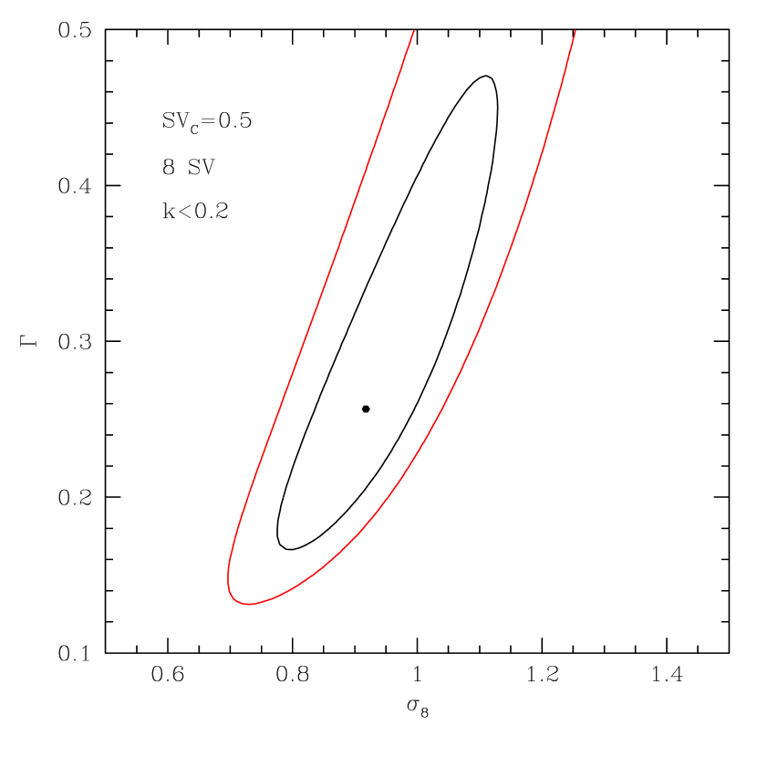
Figure 3: Constraints on a 2-parameter family of CDM power spectra when fit to the best-fit power spectrum of Table 3. Non-linear theoretical power spectra are used (Peacock & Dodds, 1996). ${\mathbf{P}}^{\prime}$ and $C_{w}$ are calculated using the observed $P_{2}$ values (eq. 27). $W_{j}$ less than $SV_{C}=0.5$ have been increased to 0.5 in constructing $C_{w}$, and only the first 8 SV modes have been included in ${\mathbf{P}}^{\prime}$. All SV modes are used in $C_{w}$. The difference between this reconstruction and the model is then used to find $\chi^{2}$. 68% and 95% contours ($\Delta\chi^{2}=2.30$ and 5.41) are shown. Only wavenumbers $k<0.2h{\rm\,Mpc}^{-1}$ are used; we marginalize over the uncertainty at larger wavenumbers.

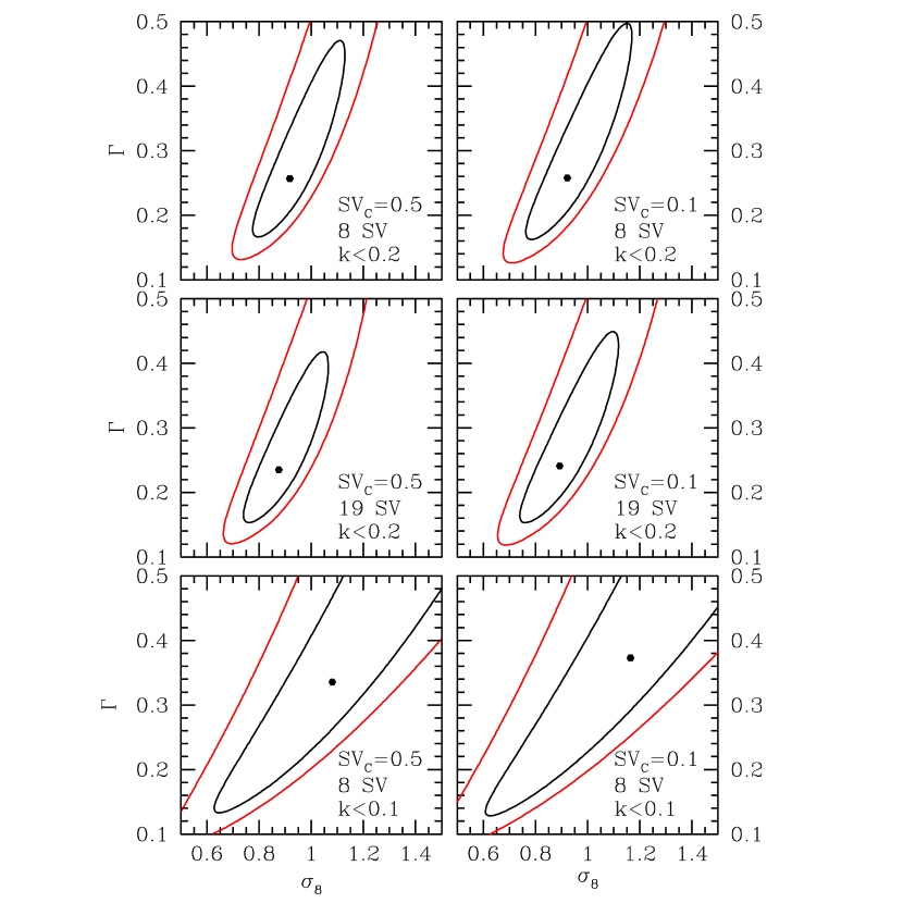
Figure 4: As Figure 3 but with changes to parameters of the reconstruction and fit. (left panels) $W_{j}$ less than $SV_{C}=0.5$ are increased to 0.5. (right panels) $W_{j}$ less than $SV_{C}=0.1$ are increased to 0.1. (top panels) Only the 8 modes with the largest $W_{j}$ are used in constructing the power spectrum. All modes are used in constructing the covariance matrix. Only wavenumbers $k<0.2h{\rm\,Mpc}^{-1}$ are used; we marginalize over the uncertainty at larger wavenumbers. (middle panels) As top, but all 19 SV are used in constructing the power spectrum. (bottom panels) As top, but only $k<0.1h{\rm\,Mpc}^{-1}$ is used.

In Figure 3, we show the constraints on these CDM models. We use $SV_{C}=0.5$ and include 8 modes in calculating ${\mathbf{P}}$. All modes are used in calculating $C_{P}$. The contours are drawn at $\Delta\chi^{2}=2.30$ and 5.41, which are the values for a 68% and 95% confidence region in a Gaussian ellipse. The constraints are rather loose. The most likely model has $\Gamma=0.26$ and $\sigma_{8}=0.92$. If we marginalize over $\sigma_{8}$, $\Gamma$ has a range of 0.19–0.37 (68%) and 0.15–0.58 (95%). The strong skewness of the constraint region towards higher $\Gamma$ is an artifact of using $\Gamma$ as a parameter. Increasing $\Gamma$ removes large-scale power, but since the error bars are not changing with $\Gamma$, eventually a small change in power maps to a large change in $\Gamma$. Because of this skew tendency, we are not generally concerned about modest changes in the upper limit on $\Gamma$ range, as they correspond to small changes in the actual power.

If we use all 19 SV modes in constructing ${\mathbf{P}}$, the $\chi^{2}$ for the best-fit CDM model is 6. This is based on 11 degrees of freedom, as calculated from 13 $k$ bins and 2 parameters. Alternatively, one can think of this as 19 $k$ bins and 8 parameters: the 2 CDM parameters at $k<0.2h{\rm\,Mpc}^{-1}$ and 6 bins of bandpower at $k>0.2h{\rm\,Mpc}^{-1}$ that have been marginalized over. $\chi^{2}=6$ on 11 degrees of freedom is small but not statistically abnormal. We would therefore say that the CDM model is an acceptable fit to the data.

If one uses only 8 SV modes to construct ${\mathbf{P}}$, the best-fit CDM model has $\chi^{2}=0.5$. One might imagine that with 8 modes and 8 parameters, one has zero degrees of freedom. However, the other 11 modes haven’t been removed from the $\chi^{2}$; they have simply had their amplitude in ${\mathbf{P}}$ set to zero. If all of the models had zero overlap with the omitted modes, then we would indeed lose one degree of freedom per frozen mode. However, the overlap is small—because the omitted modes are wiggly while the models are smooth—but non-zero. Hence, we do not find the small $\chi^{2}$ to be surprising, but it is difficult to say this quantitatively.

One might worry that allowing the power at $k>0.2h{\rm\,Mpc}^{-1}$ to vary within its errors could cause great uncertainty on large scales because we haven’t included any angular data on scales below $0^{\circ}.5$. One way to address this is to force the small-scale power spectrum to a smooth form. Holding the power at $k>0.36h{\rm\,Mpc}^{-1}$ equal to a $k^{-1.3}$ power law of unknown amplitude has only a small effect on the allowed region for $\Gamma$. Extending this power-law to $k=0.2h{\rm\,Mpc}^{-1}$ causes the confidence intervals on $\Gamma$ to be 0.19–0.33 (68%) and 0.155–0.50 (95%). This is a minor improvement for such a strong prior. As second test, we attempt to include our knowledge of the small-scale power spectrum directly in the inversion by replacing the DG99 $w(\theta)$ at $\theta<2^{\circ})$ with a finely-sampled representation of the BE93 fitting form to $w(\theta)$ that extends to $0^{\circ}.07$. This yields confidence regions on $\Gamma$ of 0.185-0.36 (68%) and 0.145-0.57 (95%). Hence, we conclude that the small scales are well-enough constrained by angular data at $\theta>0^{\circ}.5$ that their uncertainties do not affect the reconstruction of the power spectrum at $k<0.2h{\rm\,Mpc}^{-1}$.

In Figure 4, we vary some of the above assumptions. The top row of the Figure shows the results as we vary $SV_{C}$. The left panel is $SV_{C}=0.5$, as in Figure 3. In the right panel, we use $SV_{C}=0.1$. This gives the ill-constrained directions in the power spectrum fit 5 times more freedom. Indeed, their amplitudes will commonly exceed unity, which is unphysical for a positive-definite quantity like the power spectrum. The constraints on CDM parameters are slightly worse, but not considerably so. Reducing $SV_{C}$ even more makes little difference. Increasing $SV_{C}$ above 1.0 begins to shrink the allowed region and move the best-fit point to higher $\Gamma$. This is because the modes with $W_{j}\gtrsim 2$ contribute little large-scale power; if all the modes with smaller SV are suppressed by setting $W_{j}=SV_{C}$, then the result becomes biased toward zero power on large scales.

The middle row of Figure 4 shows the results when all SV are included in calculating the best-fit power spectrum. Generally the differences are small, showing that these smaller SV have little effect on fits to CDM models. Larger $\Gamma$ are slightly less favored, but the constraints are still very broad. One should remember that since the small $W_{j}$ have been increased to $SV_{C}$ before being added to ${\mathbf{P}}$, adding such modes is not more “correct” in the sense of yielding an unbiased estimator or returning the best-fit (and non-positive) power spectrum.

The bottom row of Figure 4 restricts the fit to even larger scales, $k_{c}=0.1h{\rm\,Mpc}^{-1}$. The constraints are considerably worse: in particular, no interesting upper bound can be set on $\Gamma$. The best-fit $\Gamma$ is also higher.

With $k_{c}=0.2h{\rm\,Mpc}^{-1}$, the tilt of the constraint region in the $\Gamma$–$\sigma_{8}$ plane is in the sense of a tight constraint on the rms fluctuations on a larger scale. That is, if we were to plot the constraint on the $\Gamma$–$\sigma_{24}$ plane, the region would be roughly perpendicular to the axes. This is not surprising, because $\sigma_{8}$ is dominated by $k\approx 0.2h{\rm\,Mpc}^{-1}$, and the fit should focus on larger scales.

Our fit to the observed $P_{2}$ approaches a constant as $K\rightarrow 0$, which means that it does not approach scale-invariance ($P_{2}\propto K$) on the largest scales. One might worry that this causes an overestimate of the errors on large scales. We can address this by using a CDM power spectrum when calculating $C_{w}$. We take a model with $\Gamma=0.25$ and $\sigma_{8}=0.89$ and project the non-linear $P_{3}$ to $P_{2}$. While the CDM $P_{2}$ does eventually go to zero at large scales, it actually exceeds our fit to observations at $K=10$. Using the CDM $P_{2}$ to calculate $C_{w}$, we find constraints in the $\Gamma$–$\sigma_{8}$ plane that are a very close match to those in Figure 4. In detail, the best-fit $\Gamma$ and the confidence intervals shift by only 0.01, which is far within the errors.

When fitting to cosmological models, one can include the fact that the sample-variance portion of the covariance matrix depends on the model itself. For example, one might worry that large $\Gamma$ models would predict smaller sample variance and hence be less favored than Figure 3 would suggest. We therefore repeat our fits to CDM models, using the model at each point to generate the covariance matrix and the best-fit power spectrum. We then calculate $\chi^{2}$ as before. We find that the confidence regions are essentially unchanged and that the best-fit $\Gamma$ moves by less that 0.01.

5.3 Higher-order terms in the Covariance

In our treatment so far, we have only included the Gaussian terms in the covariance matrix $C_{w}(\theta,\theta^{\prime})$. We want to estimate the size of the non-Gaussian terms and determine if their inclusion could substantially change our results. To do this, we will use the hierarchical ansatz for the higher-order moments of the density field. The four-point function is assumed to be

$$T_{4}({{\vec{K}}}_{1},{{\vec{K}}}_{2},{{\vec{K}}}_{3},{{\vec{K}}}_{4}) = r_{a}\left[P_{2}({\vec{k}}_{1})P_{2}({{\vec{K}}}_{2})P_{2}({{\vec{K}}}_{13})+{\rm cyc.}\right]+$$ (29)

$$r_{b}\left[P_{2}({\vec{k}}_{1})P_{2}({{\vec{K}}}_{2})P_{2}({{\vec{K}}}_{3})+{\rm cyc.}\right],$$

where $r_{a}$ and $r_{b}$ are constants describing the hierarchical amplitudes for the two different topologies of diagrams contributing to the four-point function. With the same set of approximations we used to obtain equation (21), the full covariance of $w(\theta)$ is

$$C_{w}(\theta,\theta^{\prime}) = {1\over A_{\Omega}}\left[\int_{0}^{\infty}{dK\,K\over 2\pi}\ 2\ P_{2}^{2}(K)J_{0}(K\theta)J_{0}(K\theta^{\prime})+\right.$$

$$\left.\int_{0}^{\infty}{dK\,K\over 2\pi}\int_{0}^{\infty}{dK^{\prime}\,K^{\prime}\over 2\pi}\bar{T}_{4}(K,K^{\prime})J_{0}(K\theta)J_{0}(K^{\prime}\theta^{\prime})\right],$$

$$\bar{T}_{4}(K,K^{\prime}) = \int{d^{2}K_{a}\over A_{r}}\int{d^{2}K_{b}\over A^{\prime}_{r}}T_{4}({{\vec{K}}}_{a},-{{\vec{K}}}_{a},{{\vec{K}}}_{b},-{{\vec{K}}}_{b}).$$ (30)

The last integral is an angular average of the four-point function over rings in $K$ space of area $A_{r}$ centered around $K$ and $K^{\prime}$.

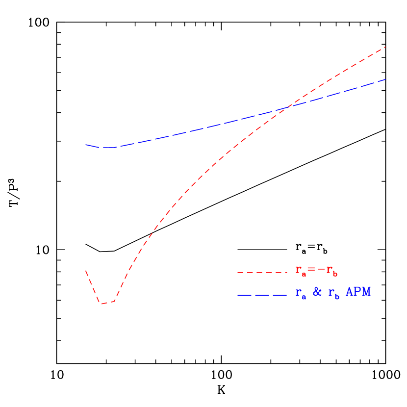
Figure 5: $T(K,K)/P_{2}^{3}(K)$ in the hierarchical model for different choices of $r_{a}$ and $r_{b}$. The hierarchical amplitudes measured from APM (Szapudy & Szalay, 1997) are expected to be larger than the amplitudes relevant for the configurations that determine the variance of the power spectrum. The curves for $r_{a}=\pm r_{b}$ are each normalized to the $T/P^{3}$ values ($R=4[2r_{a}+r_{b}]=12$) calculated when the spatial quantities obtained in $N$-body simulations were projected to the angular quantities using the APM selection function.

In order to estimate the size of this contributions we need to have an estimate of the hierarchical amplitudes $r_{a}$ and $r_{b}$. Szapudy & Szalay (1997) estimated these amplitudes for APM by measuring two different configurations of the four-point function. They obtained $r_{a}=1.15$ and $r_{b}=5.3$. The diagonal terms $\bar{T}_{4}(K,K)$ are determined mainly by the combination $R=4(2r_{a}+r_{b})=30.4$. In Scoccimarro et al. (1999), it was shown that the hierarchical ansatz is not a particularly good approximation for the configurations of the four-point function relevant for the variance of the power spectrum (or the two-point function), i.e. those configurations in which two pairs of ${\vec{K}}$ add up to zero. The amplitudes of the important configurations were roughly a factor of five smaller than one would naively expect. Therefore a smaller value of the hierarchical coefficients should be used for the variance calculation. The spatial statistics measured in particle-mesh $N$-body simulations imply after projection that the hierarchical coefficients for APM should satisfy $4(2r_{a}+r_{b})\approx 12$. Figure 5 shows the ratio of $T/P^{3}$ along the diagonal for the different choices of $r_{a}$ and $r_{b}$.

Figure 6: Cross-correlation coefficients between different $K$ shells of the angular power spectra for the choices of $r_{a}$ and $r_{b}$ listed in Figure 5. Each curve shows the cross-correlation coefficient between one $K$ shell (the one with $r_{ij}=1$) and all the rest.

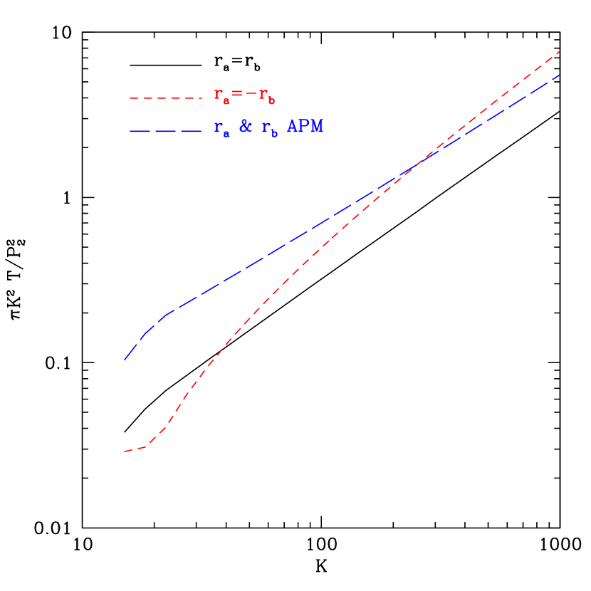
Figure 7: Ratio of the non-Gaussian terms to the Gaussian terms in the diagonal elements of the covariance matrix of the angular power spectra. We see that the non-Gaussian terms are subdominant for $K<100$.

In reality, the four-point function has other contributions due to shot noise, but in the case of APM they are subdominant for the scales of interest. The full four-point function can be written as

$$\bar{T}_{4}^{full}(K,K^{\prime})={1\over{\bar{n}}^{3}}+{2\over{\bar{n}}^{3}}[P_{2}(K)+P_{2}(K^{\prime})]+{\bar{B}(K,K^{\prime})\over{\bar{n}}}+\bar{T}_{4}(K,K^{\prime})$$ (31)

where $\bar{B}$ is the averaged bispectrum over the shells. The scaling of the three- and four-point functions with the power spectrum means that each of the additional terms coming from shot noise are down by a factor $P_{2}(K)\bar{n}$, which is smaller than one for the measured APM power spectra up to $K\approx 1000$.

In Figure 6, we show the correlation coefficients for the power spectra for the different choices of $r_{a}$ and $r_{b}$. The hierarchical model for the four-point function does not guarantee that the correlation coefficient stays smaller than unity, illustrating that this model cannot describe correctly the correlations induced by gravity. Only the case $r_{a}=-r_{b}$ makes the coefficients stay smaller than one, but Scoccimarro et al. (1999) show that the shape of the correlation coefficients in the simulations are not particularly well fitted by this choice. The hierarchical model does give a good estimate of the order of magnitude of the correlations but cannot account for their shape; this can also be seen in the results of Meiksin et al. (1999a). In summary, our calculation of the non-Gaussian effects should be taken as an order of magnitude estimate.

Figure 7 shows the ratio of the Gaussian to the non-Gaussian terms in the covariance of the angular power spectrum. We conclude that the two contributions are about equal at $K=100$, corresponding approximately to $1^{\circ}$. On the $10^{\circ}$ scale, we expect the inclusion of the four-point function in $C_{w}$ to alter the error bars by less than 10%.

A quick estimate of the effect of four-point terms on the errors of the correlation function can be obtained using a simple approximation. The four-point function scales as $P_{2}^{3}$, so we approximate $T_{4}(K,K^{\prime})$ as $R{\bar{P}_{2}}P_{2}(K)P_{2}(K^{\prime})$, where we have introduced a mean power ${\bar{P}_{2}}$. With this simplification, the non-Gaussian term in $C_{w}(\theta,\theta^{\prime})$ is $A_{\Omega}^{-1}R{\bar{P}_{2}}w(\theta)w(\theta^{\prime})$. In other words, we simply add a overall random fluctuation in the amplitude of the correlation function, $\hat{w}(\theta)=(1+\epsilon)w(\theta)$, with an rms amplitude of

$$\left<\epsilon^{2}\right>^{1/2}=0.05\left({R\over 12}\ {\bar{P}_{2}\over 2\times 10^{-4}}\ {1\ {\rm sr}\over A_{\Omega}}\right)^{1/2}.$$ (32)

This model reflects the tendency of modes to become extremely correlated in the non-linear regime, such that the shape of the power spectrum or correlation function becomes far better determined than the amplitude.

Taking $\sqrt{R{\bar{P}_{2}}}=0.05$, we add this additional correlation to $C_{w}$ and repeat the calculation of the power spectrum. The errors on $\Gamma$ increase by about 7%. If we double the amplitude of the effects to $\sqrt{R{\bar{P}_{2}}}=0.1$, the errors on $\Gamma$ increase by about 30%. We expect that this amplitude is an overestimation of the non-Gaussian corrections. The best-fit power spectra for these two cases yield fits to the observed $w(\theta)$ with $\chi^{2}=42$ and $34$, respectively, on 32 degrees of freedom. Weakening the off-diagonal terms of the non-Gaussian portion of $C_{w}$, so as to step away from total correlation between different $\theta$, causes a less severe degradation in the constraints on $\Gamma$. We therefore conclude that non-Gaussianity should have a relatively mild effect on our analysis of APM.

5.4 Lower Bound on Large-Scale Constraints from Angular Data

One can set a lower bound on the errors of an angular survey by working directly from the angular power spectrum. For a Gaussian random field with angular power spectrum $P_{2}(K)$, the covariance matrix of the angular power spectrum measured over the full sky is diagonal, with an variance equal to $2P_{2}^{2}(K)/2K\Delta K$ for a bin of width $K$. We take the optimistic assumption that a survey of sky coverage of $A_{\Omega}$ steradians will retain this variance with a scaling of $4\pi/A_{\Omega}$. We can use the transformation in equation (4) to convert the inverse covariance matrix of the angular power spectrum into that of the spatial power spectrum. The element relating two bins in spatial wavenumber is

$$C_{P}^{-1}(k,k^{\prime})=dk\,dk^{\prime}\int{dK\over K}{A_{\Omega}\over 4\pi}{1\over P_{2}^{2}(K)}f(K/k)f(K/k^{\prime}),$$ (33)

where $f(r_{a})$ is the survey projection kernel and the bins have width $dk$ and $dk^{\prime}$. To compare two spatial power spectra that differ by $\Delta P(k)$, we integrate $C_{P}^{-1}$ to find $\chi^{2}$:

$$\chi^{2}=\int dk\int dk^{\prime}\Delta P(k)\Delta P(k^{\prime})C_{P}^{-1}(k,k^{\prime}).$$ (34)

Defining

$$\Delta P_{2}(K)={1\over K}\int dkf(K/k)\Delta P(k)$$ (35)

as the angular power spectrum corresponding to the projection of the difference of the spatial power spectra, we find

$$\chi^{2}={A_{\Omega}\over 4\pi}\int dK\,K\left(\Delta P_{2}(K)\over P_{2}(K)\right)^{2}.$$ (36)

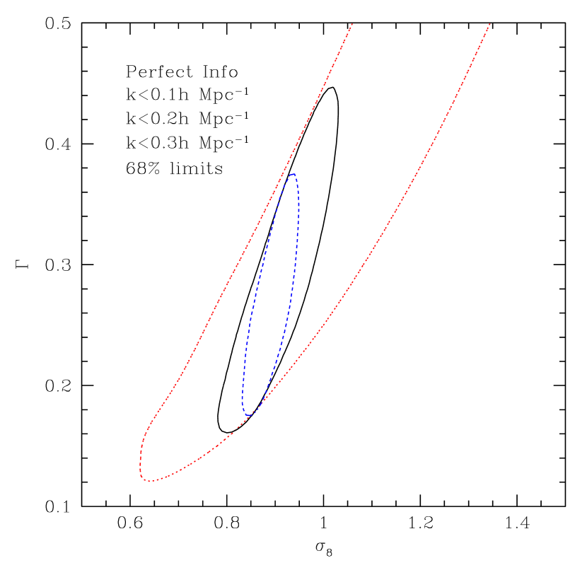
Figure 8: The constraints on CDM parameters within the APM survey if one adopts the optimistic assumptions of Equation (36). A $\Gamma=0.25$, $\sigma_{8}=0.89$ model is used to calculate the sample-variance, and the $\chi^{2}$ is calculated for the difference between this model and the grid of other models. We use non-linear spatial power spectra in all cases. We compare the CDM models only at scales larger than $0.1h{\rm\,Mpc}^{-1}$ (dotted), $0.2h{\rm\,Mpc}^{-1}$ (solid), and $0.3h{\rm\,Mpc}^{-1}$ (dashed); smaller scales are assumed to be known perfectly but to contain no extra cosmological information. This is the optimistic assumption for the extraction of the large-scale power spectrum; allowing the small scales to vary within their errors would worsen the constraints. We view the regions as lower limits on the uncertainty on the large-scale power spectrum from APM, save for the minor adjustments that would occur with a likelihood analysis on the actual data.

We now apply this limit to the CDM parameter space in the case of APM. We assume that the true clustering is given by a $\Gamma=0.25$, $\sigma_{8}=0.89$ model with non-linear evolution (Peacock & Dodds, 1996). We then consider how well one can constrain an excursion from this model on large scales. We therefore set $\Delta P(k)$ to be zero on scales $k>k_{c}$ and equal to the difference between two CDM models (the model to be tested and the $\Gamma=0.25$ model) on larger scales. This corresponds to the limit in which the small scales are considered to be perfectly known and not allowed to vary within their errors. Of course, it also assumes that this perfect knowledge on small scales says nothing to distinguish CDM models, but we are interested here in the cosmological information available in the large-scale clustering. The integral in $K$ is extended from 1 to 1000.

Figure 8 shows the constraints in the $\Gamma$–$\sigma_{8}$ plane available at scales $k<0.1h{\rm\,Mpc}^{-1}$, $k<0.2h{\rm\,Mpc}^{-1}$, and $k<0.3h{\rm\,Mpc}^{-1}$ using the sky coverage and redshift distribution of the APM survey. The ranges of allowed $\Gamma$ for the $k<0.2h{\rm\,Mpc}^{-1}$ case are 0.19–0.35 (68%) and 0.15-0.56 (95%); the best-fit is $\Gamma=0.25$ by construction. This is very similar to the limit assigned to the fit to the power spectrum reconstructed from the actual data if we use the same CDM model to generate $C_{w}$. We conclude that a survey with the sky coverage and selection function of APM has too much sample variance to place strong constraints on the shape of the power spectrum on scales greater than $k=0.1h{\rm\,Mpc}^{-1}$.

While one cannot prove it rigorously, we do not see how one could in practice achieve errors smaller than the limits implied by equation (36) and shown in Figure 8. The relevant assumptions of Gaussianity, freedom from boundary effects, infinitesimal bins in angle and wavenumber, total angular coverage, and perfect information at small scales are all optimistic. The only subtlety is that equation (36) is a statement about the $\chi^{2}$ difference between two models, whereas for the actual survey one is concerned with the likelihood function for model fits to the data. This can cause small differences if the likelihood function is non-Gaussian; in this case, the tendency would be to shift the allowed region towards larger power, i.e. smaller $\Gamma$ and larger $\sigma_{8}$.

5.5 Comparison to Previous Work

Despite the limit described in the last section, previous analyses have found substantially smaller error bars on the large-scale power spectrum. In this section, we describe how neglect of correlations and improper use of smoothing have led to these underestimates.

We would like to compare the covariance matrix derived from theory in § 3 to that used in previous analyses of the power spectra inferred from APM angular clustering. Generally, the errors for large-scale correlations have been estimated as the deviation between four subsamples of the APM survey (Maddox et al., 1996; Baugh & Efstathiou, 1993). This procedure is at best marginal for estimating even the diagonal elements of the covariance matrix, but it is completely inadequate for estimating the full covariance matrix. Indeed, one could only generate four non-zero eigenvalues! Therefore, the covariance matrices of either the angular correlations or the spatial power spectra have been assumed to be diagonal. Neither of these approximations is correct or, as we will see, particularly good.

We begin with the angular correlation function. Without the correlations between bins, it is very easy to overestimate the power of the data set by using too fine a binning in $\theta$. Neighboring bins that are highly correlated will show the same dispersion between the subsamples, but one will count this as two independent measurements rather than one. The errors on any fit will improve by $\sqrt{2}$. The visual cue that this is occurring is when the subsamples show coherent fluctuations around the mean rather than rapid bin-to-bin scatter. This is clearly occurring in Figure 27 of Maddox et al. (1996).

We can compare our calculation of $C_{w}$ to the quoted observational errors by setting all of our off-diagonal terms to zero. We then substitute this new $C_{w}$ and recalculate limits on $\Gamma$ and amplitude in the manner described in the previous section. We do the same for a diagonal $C_{w}$ that uses the errors on $w(\theta)$ based on the dispersion between 4 subsamples of APM (Maddox et al., 1996; Dodelson & Gaztañaga, 1999). As shown in Figure 9, these two choices give constraint regions that are quite similar to one another. The fact that these two treatments give similar results is evidence that sample variance in the Gaussian limit does explain most of the observed scatter in $w(\theta)$ on large angular scales in APM and further justifies the approximations that underlie our estimation of $C_{w}$.

Importantly, both diagonal treatments give constraints on CDM parameters that are a factor of two tighter than those found when using the theoretical covariance matrix with its off-diagonal terms. For example, comparing the 68% semi-range on $\Gamma$, we find 0.09 in the full $C_{w}$ case and 0.043 in either of the diagonal counterparts. The best-fit $\Gamma$ in the diagonal cases are around 0.3, somewhat higher than in the analysis with non-zero correlations in $w(\theta)$ and suggesting a bias in the reconstruction.

It should also be noted that when either of these diagonal covariance matrices are used, the $\chi^{2}$ for the $w(\theta)$ of the best-fit power spectra is less than 3 for 32 degrees of freedom. This is another indication that these matrices do not properly describe the error properties of the data.

DG99 reconstruct the power spectrum based on a diagonal covariance matrix. However, they obtain limits using $k<0.124h{\rm\,Mpc}^{-1}$ that are tighter than what we show for $k<0.2h{\rm\,Mpc}^{-1}$ in Figure 9. We believe that this is caused by the way in which their smoothing prior enters the calculation of the covariance matrix, namely that the quoted covariance matrix is for the smoothed estimator of the power not the actual power itself. On scales where the constraints from the data are poor, the smoothing prior will choose a value of the power based on an extrapolation from the wavenumbers with stronger measures of the power. The variance between samples of this extrapolated power will be far smaller than the true uncertainty in the power. We think that this underestimate of the errors at large scales is responsible for the discrepancy between the SVD treatment and the method of DG99. Indeed, DG99 found that the errors on cosmological parameters increase as they relaxed the smoothing prior.

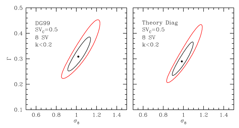
Figure 9: Constraints when the covariance matrix $C_{w}$ is assumed to be diagonal. (left panel) Observed APM error bars (Maddox et al., 1996; Dodelson & Gaztañaga, 1999) formed into a diagonal covariance matrix. (right panel) Covariance matrix from § 3, but with the off-diagonal terms set to zero. In each case, we use $SV_{C}=0.5$, consider only the largest 7 SV when constructing ${\mathbf{P}}^{\prime}$, and use only wavenumbers $k<0.2h{\rm\,Mpc}^{-1}$ in the fit. These constraints should be compared to those of Figure 3.

Baugh & Efstathiou (1993, 1994) did not use the covariance on $C_{w}$; instead they estimated errors on $P(k)$ directly by using the variance of the power spectra of the 4 subsamples, having inverted each separately. Again, 4 subsamples was too few to estimate the off-diagonal terms of $C_{P}$. It is clear, however, that these terms are important, as Figure 9 of BE93 reveals that the $P(k)$ from the 4 subsamples do show obvious correlations in their differences from the mean. The tests on simulations in Gaztañaga & Baugh (1998) also neglect the correlations between different bins in the reconstructed power spectra.

Unfortunately, we cannot simply use the diagonal terms of our $C_{P}$ matrix to compare to the BE93 results, because the inversion procedure of BE93 includes an implicit smoothing prescription. In order to compare to their estimate of the errors on the smoothed power spectrum, we would need to project our $C_{P}$ matrix onto their allowed basis, removing the variance in any disallowed directions in $P$-space. Without this step, the large variances we included for the ill-constrained directions will give enormous variance to individual $k$ bins when the detailed correlations between bins are discarded.

One must be especially wary of estimating error bars from the variance between subsamples when a smoothing prior has been applied to a wavenumber or angle where the data is not constraining. In the present context, the Lucy inversion method employed by BE93 contained a smoothing step that pushed $P(k)$ to a particular functional form. When such a method is used on large scales where the power is not well-constrained, then all subsamples will tend to reconstruct a power spectrum value on large scales that is simply an extrapolation of the smaller scale result. The dispersion between the subsamples will not grow with scale as fast as they would in the absence of smoothing, causing the resulting error bars to be significantly underestimated on large scales. We suspect that this effect is a significant contribution to why Baugh & Efstathiou (1993) find near constant power and small errors at $k<0.05h{\rm\,Mpc}^{-1}$.

6 Conclusion

Both the angular correlation function and the spatial power spectrum inferred from angular clustering have important correlations between different bins of angle and wavenumber even if the fluctuations are Gaussian. Previous analyses of the deprojection of angular clustering have neglected these effects. In this paper, we have shown how to include sample variance in the covariance matrix for the angular correlation function $w(\theta)$ under a Gaussian, wide-field approximation. We have then described how one may invert $w(\theta)$ to find the spatial power spectrum using singular value decomposition in such a way as to retain the full covariance matrix. The method allows one to handle the near-singularity of the projection kernel without numerical difficulty and can yield a smoothed version of the deprojected power spectrum without sacrificing the covariances of unsmoothed spectrum.

Using the large-angle galaxy correlations of the APM survey as an example, we have shown that correlations between different bins in $\theta$ and in $k$ are critical for quoting accurate statistical limits on the power spectrum and model fits thereto. With the sample variance properly included, we find that APM does not detect a downturn in $P(k)$ at $k<0.04h{\rm\,Mpc}^{-1}$; the significance is only 1–$\sigma$. Fitting non-linearly extrapolated, scale-invariant CDM power spectra to the power spectrum at large scales ($k<0.2h{\rm\,Mpc}^{-1}$), we find that APM constrains the CDM parameter $\Gamma$ to be 0.19–0.37 (68%). We have investigated a wide range of alterations to the method in the hopes of shrinking this range but have found nothing that makes a significant difference. Indeed, in § 5.4, we showed that the above constraints already approach the best available to a survey with the sky coverage and selection function of APM. Extending the CDM fits to smaller scales would improve the constraints, but this depends entirely on the modeling of galaxy bias and non-linear gravitational evolution. Moreover, such a fit wouldn’t validate this particular set of CDM models because many other models would look similar in the non-linear regime. To confirm a model from galaxy clustering, one would like to see the characteristic features of the model directly rather than attempt to leverage a measurement of the slope in the non-linear regime onto a cosmological parameter space.

We have made a number of approximations in our analysis. In our treatment of large scales, we have ignored the ability of boundaries to alias power from one scale to another and used Limber’s equation even for modes with wavelengths similar to the scale of the survey. On small scales, we have ignored three-point and four-point contributions to the covariance matrix of the angular statistics. In general, we have treated the likelihood of the correlation function as a Gaussian and ignored the fine details of how cosmology or evolution of clustering might enter. We have argued that the above approximations are likely to be reasonably accurate for an analysis of the large-angle clustering of APM. We also have not questioned the redshift distribution function that has been used in past APM analyses nor included any systematic errors. Conservatively, therefore, one can regard our results as the optimistic limits, because it is very unlikely that the breakdown of any of the above assumptions would actually improve the constraints!

Surveys such as DPOSS and SDSS will be substantially deeper and wider than the APM survey. We repeat the analysis of § 5.4 for parameters suggestive of SDSS, namely 3.1 steradians of sky coverage to a median redshift of 0.35. This yields an error on $\Gamma$ of 0.017 (1–$\sigma$) about a fiducial model of $\Gamma=0.25$. Remember that this is an optimistic limit on the error, that we have assumed perfect knowledge of the selection function, and that we have only allowed one other parameter, the amplitude, to vary! With analogous assumptions, the limit on $\Gamma$ from the SDSS redshift survey of bright red galaxies is roughly 0.007. The redshift survey would be more strongly preferred if one were interested in narrower features in the power spectrum (Meiksin et al., 1999b), such as would be needed to separate effects in a larger parameter space (Eisenstein et al., 1999). As regards systematic errors, the angular survey suffers from its dependence on purely tangential modes, while the redshift survey must contend with redshift-space distortions.

If one could use color information to select a clean, high-redshift sample of galaxies, the prospects for interpreting angular correlations improve. For example, using only those galaxies with $z>0.45$ in the above SDSS example drops the limiting errors on $\Gamma$ to 0.010. This occurs because the obscuring effects of smaller-scale clustering from lower redshift galaxies have been removed; moreover, the projection from three dimensions to two becomes significantly sharper. This performance is comparable to that of the redshift survey and would allow measurement of the large-scale power spectrum in a range of redshifts disjoint from the spectroscopic survey, thereby allowing one to study the evolution of large-scale clustering.

The results of this paper, and particularly the limits set in § 5.4, provide a cautionary note for the interpretation of large angular surveys. Even at the depths of the SDSS imaging, the constraints on large-scale clustering from angular correlations alone are not strong. The inclusion of photometric redshifts to separate the sample into multiple (or even continuous) radial shells could provide a significant improvement to this state of affairs.

References

- Baugh & Efstathiou (1993) Baugh, C.M., & Efstathiou, G. 1993, MNRAS, 265, 145 (BE93)
- Baugh & Efstathiou (1994) Baugh, C.M., & Efstathiou, G. 1994, MNRAS, 267, 323
- Dodelson & Gaztañaga (1999) Dodelson, S., & Gaztañaga, E. 1999, preprint [astro-ph/9706018] (DG99)
- Djorgovski et al. (1998) Djorgovski, S.G., Gal, R.R., Odewahn, S.C., de Carvalho, R.R., Brunner, R., Longo, G., & Scaramella, R. 1998, Wide Field Surveys in Cosmology, eds. S. Colombi & Y. Mellier [astro-ph/9809187]
- Eisenstein et al. (1999) Eisenstein, D.J., Hu, W., & Tegmark, M. 1999, ApJ, 518, 2
- Gawiser & Silk (1998) Gawiser, E., & Silk, J. 1998, Science, 280, 1405
- Gaztañaga & Baugh (1998) Gaztañaga, E., & Baugh, C.M. 1998, MNRAS, 294, 229 [astro-ph/9704246]
- Groth & Peebles (1977) Groth, E.J., & Peebles, P.J.E., 1977, ApJ, 217, 592
- Hamilton (1999) Hamilton, A.J.S., 1999, MNRAS, in press [astro-ph/9905192]
- Limber (1953) Limber, D.N. 1953, ApJ, 117, 134
- Maddox et al. (1990) Maddox, S.J., Sutherland, W.J., Efstathiou, G., & Loveday, J. 1990, MNRAS, 242, 43p
- Maddox et al. (1996) Maddox, S.J., Efstathiou, G., & Sutherland, W.J. 1996, MNRAS, 283, 1227
- Meiksin et al. (1999a) Meiksin, A., & White, M., 1999, MNRAS, 308, 1179
- Meiksin et al. (1999b) Meiksin, A., White, M., & Peacock, J.A., 1999, MNRAS, 304, 851
- Peacock & Dodds (1996) Peacock, J.A., & Dodds, S.J., 1996, MNRAS, 280, L19
- Peebles (1973) Peebles, P.J.E. 1973, ApJ, 185, 413
- Phillips et al. (1978) Phillips, S., Fong, R., Ellis, R.S., Fall, S.M., MacGillivray, H.T. 1978, MNRAS, 182, 673
- Press et al. (1992) Press, W.H., Teukolsky, S.A., Vetterling, W.T., & Flannery, B.P. 1992, Numerical Recipes, 2nd edition (Cambridge: Cambridge Univ. Press), §§2.6, 15.6
- Scoccimarro et al. (1999) Scoccimarro, R., Zaldarriaga, M., & Hui, L., 1999, preprint [astro-ph/9901099]
- Scott et al. (1994) Scott, D., Srednicki, M., & White, M., 1994, 421, L5
- Szapudy & Szalay (1997) Szapudi I. & Szalay A., 1997, ApJ, 481, L1