CMB Anisotropy in Compact Hyperbolic universes I: Computing Correlation Functions

Abstract

CMB anisotropy measurements have brought the issue of global topology of the universe from the realm of theoretical possibility to within the grasp of observations. The global topology of the universe modifies the correlation properties of cosmic fields. In particular, strong correlations are predicted in CMB anisotropy patterns on the largest observable scales if the size of the Universe is comparable to the distance to the CMB last scattering surface. We describe in detail our completely general scheme using a regularized method of images for calculating such correlation functions in models with nontrivial topology, and apply it to the computationally challenging compact hyperbolic spaces [1, 2]. Our procedure directly sums over images within a specified radius, ideally many times the diameter of the space, effectively treats more distant images in a continuous approximation, and uses Cesaro resummation to further sharpen the results. At all levels of approximation the symmetries of the space are preserved in the correlation function. This new technique eliminates the need for the difficult task of spatial eigenmode decomposition on these spaces. Although the eigenspectrum can be obtained by this method if desired, at a given level of approximation the correlation functions are more accurately determined. We use the 3-torus example to demonstrate that the method works very well. We apply it to power spectrum as well as correlation function evaluations in a number of compact hyperbolic (CH) spaces. Application to the computation of CMB anisotropy correlations on CH spaces, and the observational constraints following from them, are given in a companion paper.

I Introduction

The remarkable degree of isotropy of the cosmic microwave background (CMB) points to homogeneous and isotropic Freidmann-Robertson-Walker (FRW) models for the universe. The underlying Einstein’s equations of gravitation are purely local, completely unaffected by the global topological structure of space-time. In fact, in the absence of spatially inhomogeneous perturbations, a FRW model predicts an isotropic CMB regardless of the global topology.

Flat or ‘open’ FRW models adequately describe the observed average local properties of our Universe. Much of recent astrophysical data suggest the cosmological density parameter in nonrelativistic matter, $\Omega_{m}$, is subcritical [3]. The total density parameter $\Omega_{0}$ includes relativistic particles and vacuum, scalar field or cosmological constant, contributions, as well as $\Omega_{m}$. If a cosmological constant (or some other exotic smooth matter component) does not compensate for the deficit from unity, this would imply a hyperbolic spatial geometry (uniform negative curvature), commonly referred to as an ‘open’ universe in the cosmological literature. The simply connected (topologically trivial) hyperbolic 3-space ${\cal H}^{3}$ and the flat Euclidean 3-space ${\cal E}^{3}$ are non-compact and have infinite volume. There are numerous theoretical motivations, however, to favor a spatially compact universe [4, 5, 6, 7, 8]. To reconcile a compact universe with a flat or hyperbolic geometry, consideration of multiply connected (topologically non-trivial) spaces is required. (Inhomogeneous simply connected models are another way out; e.g., a hyperbolic bubble could be embedded in a highly inhomogeneous space and if the bubble is much larger than the Hubble radius we would not know.) Compact hyperbolic spaces have been recently used to construct cosmological models within the framework of string theory [9]. A compilation of recent articles describing various aspects of current research in compact cosmologies can be found in [10].

The realization that the universe with the same local geometry has many different choices of global topology is as old as modern cosmology – De Sitter was quick to point out that Einstein’s closed static universe model with spherical geometry ${\cal S}^{3}$ could equally well correspond to a multiply connected Elliptical universe model where the antipodal points of ${\cal S}^{3}$ are topologically identified. The possibility of a multiply connected universe has lingered on the fringes of cosmology largely as a theoretical curiosity (e.g., in [4]), but was sometimes invoked to explain puzzling cosmological observations (e.g., as a possible explanation for the isotropy of the CMB radiation [7], and for the (controversial) observations of periodic or discordant quasar redshifts  [11]). There is a long history of attempts to search for signatures of non-trivial global topology by identifying ghost images of local galaxies, clusters or quasars at higher redshifts [5, 6, 12]. The search for signatures of global topology in the distribution of luminous matter can probe the topology of the universe only on scales substantially smaller than the apparent radius of the observable universe. Another avenue in the search for global topology of the universe is through the effect on the power spectrum of cosmic density perturbation fields, reflected in observables such as the distribution of matter in the universe and the CMB anisotropy.

The observed large scale structure in the universe implies spatially inhomogeneous primordial perturbations existed which gave rise to the observed anisotropy of the CMB. The global topology of the universe also modifies the local observable properties of the CMB anisotropy on length scales up to a few times the horizon size. In compact universe models, the finite spatial size usually precludes the existence of primordial fluctuations with wavelengths above a characteristic scale related to the size. As a result, the power in CMB anisotropy is suppressed on large angular scales. Another consequence is the breaking of statistical isotropy in characteristic patterns determined by the photon geodesic structure of the manifold. One can search for such patterns statistically in CMB anisotropy maps. Full-sky CMB data, such as from the cobe–dmr experiment, can constrain the size of the universe and its topology to the extent that such correlation patterns are absent in the data [2, 16].

For Gaussian perturbations, the angular correlation function, $C(\hat{q},\hat{q}^{\prime})$, of the CMB temperature fluctuations in two directions $\hat{q}$ and $\hat{q}^{\prime}$ in the sky completely encodes the CMB anisotropy predictions of a model. For adiabatic perturbations, the dominant contribution to the anisotropy in the CMB temperature measured with a wide-angle beam ($\theta_{\sc fwhm}\mathrel{\hbox to0.0pt{\lower 3.0pt\hbox{$\mathchar 536\relax$}\hss}\raise 2.0pt\hbox{$\mathchar 318\relax$}}2^{\circ}~{}\Omega_{0}^{1/2}$) comes from the cosmological metric perturbations through the Sachs-Wolfe effect. The angular correlation function $C(\hat{q},\hat{q}^{\prime})$ then depends on the spatial two point correlation function, $\xi_{\Phi}\equiv\langle\Phi({\bf x},\tau_{\sc ls})\Phi({\bf x^{\prime}},\tau_{\sc ls})\rangle$, of the gravitational potential, $\Phi$, on the three-hypersurface of last scattering along the lines-of-sight, ${\hat{q}}$ and ${\hat{q}}^{\prime}$. Thus we need to learn how to compute spatial correlation functions on compact spaces.

When the eigenfunctions of the Laplacian on the space are known, the correlation function can be readily obtained via a mode sum. For this to be tractable the known eigenfunctions would, preferably, be expressed in a reasonably simple closed form. However, obtaining closed form expressions for eigenfunctions may not be possible beyond the simplest topologies. Some examples where explicit eigenfunctions have been used include flat models [17, 18, 19, 20] and a non-compact hyperbolic space with a horn topology [21]. In this paper we provide a detailed description of our regularized method of images for computing correlation functions, which does not require any prior knowledge of the eigenfunctions on the compact spaces [2, 1]. The method allows us to accurately compute the correlation function on compact spaces where eigenfunctions are not available. Most notorious in this respect are compact spaces with uniform negative curvature, the Compact Hyperbolic (CH) spaces, for which even numerical estimation of the eigenfunctions is believed to be a challenging task (for recent progress see [13, 14, 15]). A novel feature of our scheme is the regularization procedure that we devise in order to successfully implement the method of images for the power spectra of cosmological perturbations expected from early universe physics. As an additional bonus, this regularization scheme enhances the convergence properties of the method, which proves to be very useful for tackling CH spaces.

In $\S$II, we introduce compact spaces and briefly review the aspects that are relevant for our work. The method of images is derived in $\S$III. As a simple illustrative example, we apply the method of images to the case of a simple flat torus in $\S$IV. The implementation of the method in CH spaces is presented in $\S$V. The gross properties of the power spectrum in CH spaces that can be inferred from our computation is discussed in $\S$V C. We derive the properties of the correlation function in CH space in $\S$VI. In $\S$VII, we discuss our results and point to our companion paper describing our detailed CMB anisotropy calculations [16].

II Primer on Compact spaces

A Mathematical Preliminaries

A compact cosmological model ${\cal M}$ is a Quotient Space constructed by identifying points on the standard FRW spaces under the action of a suitable  discrete subgroup of motions, $\Gamma$, of the full isometry group $G$, of the FRW space (see [4, 22]). The isometry group $G$ is the group of motions which preserves the distances between points. The infinite FRW spatial hypersurface is the universal cover, ${\cal M}^{u}$, tiled by copies of the compact space, ${\cal M}$. Cosmological postulates of local homogeneity and isotropy restrict ${\cal M}^{u}$ to be a space of constant curvature – Hyperbolic ${\cal H}^{3}$, with negative curvature, Spherical ${\cal S}^{3}$, with positive curvature, or flat Euclidean ${\cal E}^{3}$, with zero curvature. The compact space for a given location of the observer is represented as the Dirichlet domain with the observer at its basepoint. Every point ${{\bf x}}$ of the compact space has an image ${{\bf x}}_{i}=\gamma_{i}{{\bf x}}$ in each copy of the Dirichlet domain on the universal cover, where $\gamma_{i}\in\Gamma$. The tiling of the universal cover with Dirichlet domains is a Voronoi tessellation (a familiar concept in cosmology that has been used in modeling the large scale structure in the universe), with the seeds being the basepoint and its images. The Dirichlet domain represents the compact space as a convex polyhedron with an even number of faces, with congruent pairs of faces identified (glued) under $\Gamma$. For more details, see e.g.,  [4, 22, 23, 6].

More explicitly, the Dirichlet domain around the basepoint, ${\bf x}_{0}$, is the set of all points on the universal cover which are closer (or equidistant) to ${\bf x}_{0}$ than to any of the images $\gamma{\bf x}_{0}$ ($\gamma\in\Gamma$) of the basepoint. The hyperplane that bisects the segment joining ${\bf x_{0}}$ to $\gamma{\bf x_{0}}$ divides ${\cal M}^{u}$ into two parts; let $H_{\gamma}$ denote that half that contains the basepoint. By definition, the Dirichlet domain around ${\bf x}_{0}$ is ${\cal D}_{{\bf x}_{0}}=\bigcap_{\gamma}H_{\gamma}$. Thus, the Dirichlet domain is bounded by hyperplanes bisecting the (geodesic) segments joining the basepoint ${\bf x}_{0}$ to a set of adjacent images. (The corresponding set of motions is called the set of adjacency transformations.) The faces of the polyhedron are identified pairwise; the one formed by the hyperplane bisecting the segment joining ${\bf x_{0}}$ to $\gamma{\bf x_{0}}$ is identified with the corresponding one bisecting the segment joining ${\bf x_{0}}$ to $\gamma^{-1}{\bf x_{0}}$. The adjacency transformations generate the group $\Gamma$ and hence are also known as the face generators.

In the context of cosmology, the Dirichlet domain constructed around the observer represents the universe as ‘seen’ by the observer. (In our papers, we will often loosely use the same notation ${\cal M}$ to refer to the compact space as well as one of its Dirichlet domain representations whose basepoint is clear from the context.) It proves useful then to define the outradius $R_{>}$ and the inradius $R_{<}$ of the Dirichlet domain [5]: the radius of the smallest sphere around the observer which encloses the Dirichlet domain and that of the largest sphere around the observer which can be enclosed within the Dirichlet domain, respectively . The ratio $R_{>}/R_{<}$ is a good indicator of the shape of the Dirichlet domain.

In cosmology, distances are inferred from the cosmological redshift which is related to the light travel time. Consequently, in compact spaces, and, more generally, in multiply connected spaces, light from the same source seems to arrive from points at different locations – the source and its images on the universal cover. Any source inferred to be at a distance greater than $R_{>}$ from the observer is bound to be the image of a point which is physically closer. On the other hand, a source closer than $R_{<}$ is definitely at its true physical distance. Note that $R_{>}$ and $R_{<}$ are specific to the location of the observer within the compact space since the Dirichlet domain around different observers can, in general, vary. An observer (and Dirichlet domain) independent linear measure of the size of the compact space is given by the diameter of the space, $d_{\!\cal M}\equiv\sup_{x,y\in{\cal M}}d(x,y)$, i.e., the maximum separation between two points in the compact space.

The isometry group $G$ defining the global symmetries of ${\cal M}$ is the centralizer of $\Gamma$ in the isometry group $G^{u}$ of its universal cover, ${\cal M}^{u}$; i.e., $G=\{g\in G^{u}|g\gamma=\gamma g\,\forall\gamma\in\Gamma\}$. In general, ${\cal M}$ respects less symmetries than ${\cal M}^{u}$; consequently, $G$ is of lower dimension than $G^{u}$. ${\cal M}$ is (globally) homogeneous if and only if $G$ is transitive on ${\cal M}$: i.e., for any two points ${\bf x},{\bf y}\in{\cal M}$, there exists a $g\in G$ such that ${\bf y}=g{\bf x}$ (an equivalent statement is that a compact space is globally homogeneous if and only if every element of $\gamma\in\Gamma$ is a Clifford translation, i.e., the displacement function, $d_{\gamma}(x)\equiv d({\bf x},\gamma{\bf x})$, is independent of ${\bf x}$ for all points ${\bf x}\in{\cal M}^{u}$). Space is isotropic (around a point, or observer, ${\bf x_{o}}$) if $G$ contains a subgroup of rotations around ${\bf x_{o}}$. The only example of a multiply connected compact universe which retains all the symmetries of its universal cover is the Elliptic space (${\cal S}^{3}/Z_{2}$) with spherical geometry; the simple flat torus is anisotropic, and all others (including the entire class of CH manifolds) break global homogeneity as well. As the result, the two-point correlation functions $\xi({\bf x,y})$ in CH spaces depend separately on both points ${\bf x}$ and ${\bf y}$, and not only on the distance $d({\bf x,y,})$ as in the familiar FRW spaces.

B Compact Euclidean spaces

The compact spaces with Euclidean geometry (zero curvature) have been completely classified. In three dimensions, there are known to be six possible topologies that lead to orientable spaces [4, 22, 23]: the simple flat torus where ${\cal E}^{3}$ is identified under a discrete group of translations; three other flat tori where the identification is under a screw motion, i.e., translation accompanied by a rotation about the direction of the translation, namely, rotation by $\pi$ or $\pi/2$ in one component of the translations, and rotation by $\pi$ in all three directions; and finally, two topologies made by identifying the planar hexagonal lattice under a screw motion perpendicular to the plane with rotation of $\pi/3$ and $2\pi/3$, respectively.

C Compact Hyperbolic spaces

For cosmological CH models, ${\cal M}^{u}\equiv{\cal H}^{3}$, the three dimensional hyperbolic (uniform negative curvature) manifold with line element

$$ds^{2}=d\chi^{2}+\sinh^{2}\chi\,(d\theta^{2}+\sin^{2}\theta d\phi^{2})\,,$$ (1)

where $\chi=(\tau_{0}-\tau)/d_{c}$ is the affine distance, $\tau$ is the conformal time and $d_{c}=cH_{0}^{-1}/\sqrt{1-\Omega_{0}}$ is the curvature radius set by the present cosmological density parameter $\Omega_{0}$ and the Hubble constant $H_{0}$. For a universe with hyperbolic geometry, $0<\Omega_{0}<1$; thus the size of $d_{c}$ ranges from $cH_{0}^{-1}$ as $\Omega_{0}\to 0$ to infinity as $\Omega_{0}\to 1$.

${\cal H}^{3}$ can be viewed as a hyperbolic section embedded in four dimensional flat Lorentzian (Minkowski) space, by representing each point on ${\cal H}^{3}$ as a unit four vector, ${\bf X}\equiv(\zeta({\bf x}),{\bf x})$, normalized by $d_{c}$ in Minkowski space ($\zeta^{2}-|{\bf x}|^{2}=d_{c}^{2}$). The distance between two points on ${\cal H}^{3}$ is given by the dot product of the corresponding four vectors. The isometry group of ${\cal H}^{3}$ is then the group of rotations in the four space, the proper Lorentz group $SO(3,1)$. A CH manifold is completely described by a discrete subgroup, $\Gamma$, of the proper Lorentz group $SO(3,1)$.

There are two remarkable features of tessellating ${\cal H}^{3}$ under a discrete group of motions that are absent in the flat geometry. Firstly, whereas in flat geometry all finite volume Quotient Spaces obtained are necessarily compact, one can tessellate ${\cal H}^{3}$ with tiles of finite volume which are non-compact, giving rise to a class of non-compact finite-volume hyperbolic universe models. Typically, these spaces have cusp-like extensions to infinity. Secondly, a given CH topological structure fits only for a specific volume of the space. This is in contrast to flat compact spaces, in which the same topological structure can be imposed on any scales. In particular, all simple flat tori with different identification lengths are homeomorphic to each other, i.e., one can be obtained from the other by a continuous mapping/deformation, but are not isometric to each other, i.e., the distance between the mapped points are not the same. Two hyperbolic spaces of finite volume which are homeomorphic are necessarily isometric (in three dimensions and above). This result, known in mathematics literature as the strong rigidity theorem, can be attributed to the existence of the intrinsic length scale on ${\cal H}^{3}$ – the curvature radius, $d_{c}$. It not difficult to convince oneself that the Dirichlet domain has to have a fixed size relative to $d_{c}$ in order to tile ${\cal H}^{3}$ – if one were to scale the polygon size (relative to $d_{c}$) then the scaled tiles will no longer fit together at the vertices.

Thus, a CH manifold, ${\cal M}$, is characterized by a dimensionless number, ${\cal V}_{\!\cal M}\equiv V_{\!\cal M}/d_{c}^{3}$, where $V_{\!\cal M}$ is the volume of the space and $d_{c}$ is the curvature radius [24]. There are a countably infinite number of CH manifolds, and no upper bound on ${\cal V}_{\!\cal M}$. The theoretical lower bound stands at ${\cal V}_{\!\cal M}\geq 5/(2\sqrt{3}){\rm Arcsinh}^{2}\left(\sqrt{3}/5\right)\approx 0.167$ [25]. The smallest CH manifold discovered so far has ${\cal V}_{\!\cal M}=0.94$ and it has been conjectured that this is, in fact, the smallest possible [26, 27]. The physical volume of the CH universe with a given topology, i.e., a fixed value of $V_{\!\cal M}/d_{c}^{3}$, is then set by $d_{c}$ and is thus related to cosmological parameters. The Geometry Center at the University of Minnesota has a large census of CH manifolds in its public domain. This census was created using the SnapPea computer software which is also freely available at the website [28]. The Minnesota census lists several thousands of these manifolds with ${\cal V}_{\!\cal M}$ up to $\sim 7$ and the SnapPea software can be used to obtain various characteristic properties of these CH manifolds such as the ones listed in Table I and also the generators of the discrete group motion $\Gamma$ that we need for our computational method.

The sequences of CH manifolds are closed well-ordered sets of order type $\omega^{\omega}$, i.e., are arranged in a countably infinite number of countably infinite sequences (in increasing volume), with each sequence having a non-compact finite volume hyperbolic space as its limit. These limit spaces of finite volume have cusps extending to infinity. The cusps are homeomorphic to $T^{2}\times R^{+}$, the product of a $2$-torus and the positive real line. The sequence of CH spaces arises through Dehn filling, a procedure which truncates the cusps of the limit space along a closed curve on $T^{2}$ (with allowed pair of winding numbers) and glues in a solid torus (by identifying the closed curve along a meridian of the solid torus). The nomenclature of CH spaces in the Minnesota census, which we follow in this work, identifies a sequence by the limit space and specifies a CH space belonging to it by two (coprime) integer indices in parenthesis correspond to the winding numbers, $m$ and $n$, which characterize the closed curve on the torus; e.g., m004(-5,1) refers to the CH manifold obtained by Dehn-filling the single cusp of the non-compact space m004 by a torus glued along a closed curve with winding numbers $(-5,1)$. The limit non-compact space is achieved as a limit of large values of the winding numbers in the corresponding sequence of CH manifolds. From the observational perspective, the CH spaces with high winding numbers should be practically indistinguishable from the limit non-compact space. The space with winding numbers $(m,n)$ is equivalent to the space $(-m,-n)$ in the same sequence. Not all integer values of $m$ and $n$ lead to a CH space, there are bounded forbidden gap regions in the $m$–$n$ lattice. One should note that the volume does not uniquely characterize a space; there can be a finite number of distinct CH spaces with the same volume (besides the mirror image pairs for chiral CH spaces such as m004(-5, 1) & m004(5, 1)). Also, the nomenclature described above is not unique: the same CH space may belong to two different sequences, e.g., the space m003(-2,3) is equivalent to m004(5,1). (See [27] for details.)

All CH hyperbolic spaces are necessarily globally inhomogeneous since the only element of $SO(3,1)$ which is a Clifford translation is the identity [22]. A short proof follows. Assume that $g\in SO(3,1)$ is a Clifford translation. Then $d({\bf x}_{1},g{\bf x}_{1})=d({\bf x}_{2},g{\bf x}_{2})$ for any two points ${\bf x}_{1}$ and ${\bf x}_{2}$ on ${\cal H}^{3}$. Since $SO(3,1)$ is the isometry group of the homogeneous space ${\cal H}^{3}$, there exists a Lorentz transformation $\Lambda\in SO(3,1)$ such that ${\bf x}_{2}=\Lambda{\bf x}_{1}$. Consequently, $d({\bf x}_{1},g{\bf x}_{1})=d(\Lambda{\bf x}_{1},g\Lambda{\bf x}_{1})$, implying that $g=\Lambda^{-1}g\Lambda$  $\forall\Lambda\in SO(3,1)$. Since the Lorentz group is non-Abelian (i.e., actions of the group elements do not commute), $g$ must be the identity.

FIG. 1.: The Dirichlet domains of two of the compact hyperbolic (CH) spaces that we have studied are shown. On the left is a small CH space, m004(-5,1), and on the right is a large CH space, v3543(2,3).

TABLE I.: The characteristics of some of the compact hyperbolic (CH) manifolds that we have studied. The nomenclature of the spaces conforms to the Minnesota census. The volume and diameter (expressed in the units of curvature radius) are topological invariants which relate to the density of states in those spaces. The specifications have been obtained from the Minnesota census using SnapPea. The exception is the diameter which is our estimate using a simple random sampling algorithm. However, in the context of cosmology, the observer specific characterization of the Dirichlet domain (around the observer) proves useful. The m003 models correspond to spaces obtained by different Dehn fillings on a (non-compact) cusped manifold, m003. The CH space m003(-3,1) has the smallest volume in the m003 series and is also currently the smallest CH space known. The m004(-5,1) has the smallest volume in the m004 series. The v3543(2,3) space is a relatively large one.

Properties	m003(-3,1)	m003(-4,3)	m003(-4,1)	m003(2,3)	m003(-5,4)	m004(-5,1)	v3543(2,3)
Topological invariants:
Volume: ${\cal V}_{\!\cal M}$	0.94	1.26	1.42	1.54	1.59	0.98	6.45
diameter: $d_{\!\cal M}$	0.84	1.01	1.10	1.16	1.21	0.86	1.90
First Homology group	$Z_{5}\oplus Z_{5}$	$Z_{5}\oplus Z_{5}$	$Z_{35}$	$Z_{35}$	$Z_{30}$	$Z_{5}$	$Z_{93}$
Dirichlet domain specific:
outradius: $R_{>}/d_{c}$	0.75	0.84	1.07	0.83	0.94	0.75	1.33
inradius: $R_{<}/d_{c}$	0.52	0.55	0.54	0.59	0.57	0.53	0.89
No. of faces	18	22	24	26	28	16	38
No. of vertices	26	40	44	48	52	16	72

III Method of Images

A The correlation function

The correlation function $\xi_{\Phi}({\bf x},{\bf x}^{\prime})$ of a scalar field, $\Phi$, can be expressed formally in terms of the orthonormal set of eigenfunctions $\Psi_{i}$ of the Laplace operator, $\nabla^{2}$, on the hypersurface (with positive eigenvalues $k_{i}^{2}\geq 0$), as [29]

$$\xi_{\Phi}({\bf x},{\bf x}^{\prime})=\sum_{i}P_{\Phi}(k_{i})\sum_{j=1}^{m_{i}}\Psi_{ij}({\bf x})\Psi_{ij}^{*}({\bf x}^{\prime})\,,\ {\rm where}\ (\nabla^{2}+k_{i}^{2})\Psi_{ij}=0\,.$$ (2)

The spectrum of the Laplacian on a compact space (thus with closed boundary conditions) is a discrete ordered set of eigenvalues $\{k^{2}_{i}\}$ ($k_{0}^{2}=0$ and $k_{i}^{2}<k^{2}_{i+1}$) with multiplicities $m_{i}$. The function $P_{\Phi}(k_{i})$ describes the rms amplitude of the eigenmode expansion of the field $\Phi$, determined in the context of cosmology by the physical mechanism responsible for the generation of $\Phi$.

Except in simple cases, neither the spectrum of the Laplacian $\{k^{2}_{i}\}$ nor the eigenfunctions $\Psi_{ij}^{c}({\bf x})$ are known for compact manifolds, so eq.(2) cannot be used to calculate the correlation function $\xi^{c}_{\Phi}({\bf x},{\bf x}^{\prime})$ on a compact manifold ${\cal M}$ directly. In contrast, the universal cover ${\cal M}^{u}$ for the compact manifold is usually simple enough (e.g., ${\cal H}^{3}$, ${\cal S}^{3}$ or ${\cal E}^{3}$) that the eigenfunctions $\Psi^{u}_{j}(k,{\bf x})$ are known and the correlation functions $\xi^{u}_{\Phi}({\bf x},{\bf x}^{\prime})$ are easily computable. We consider ${\cal H}^{3}$ and ${\cal E}^{3}$ geometries where the spectrum of eigenvalues on the universal cover ${\cal M}^{u}$ is continuous, reflected in the notation $\Psi^{u}_{j}(k,{\bf x})$ replacing the discrete index $i$ with a functional dependence on $k$.

The regularized method of images we developed in [1] allows computation of the correlation function $\xi^{c}_{\Phi}({\bf x},{\bf x}^{\prime})$ on a compact (more generally, a multiply connected) manifold ${\cal M}={\cal M}^{u}/\Gamma$ from the correlation function, $\xi^{u}_{\Phi}({\bf x},{\bf x}^{\prime})$, on ${\cal M}^{u}$. We now give the explicit derivation of the relation between $\xi^{c}_{\Phi}({\bf x},{\bf x}^{\prime})$ and $\xi^{u}_{\Phi}({\bf x},{\bf x}^{\prime})$, calculated with the same form of the power spectrum $P_{\Phi}(k)$. The method solely relies on the knowledge of the action of elements of the discrete group, $\Gamma$, and requires no information regarding the eigenvalues and eigenmodes of the Laplacian on ${\cal M}$. The expansion (2) is equivalent to the system of integral equations on the correlation functions, $\xi^{c}_{\Phi}$ and $\xi^{u}_{\Phi}$,

$$\int_{{\cal M}}d{\bf x^{\prime}}~{}\xi^{c}_{\Phi}({\bf x},{\bf x}^{\prime})~{}\Psi^{c}_{ij}({\bf x}^{\prime})=P_{\Phi}(k_{i})\Psi^{c}_{ij}({\bf x})\,,$$ (4)

$$\int_{{\cal M}^{u}}d{\bf x^{\prime}}~{}\xi^{u}_{\Phi}({\bf x},{\bf x}^{\prime})~{}\Psi^{u}_{j}({k,\bf x^{\prime}})=P_{\Phi}(k)\Psi^{u}_{j}(k,{\bf x})\,.$$ (5)

Eq.(5) is a consequence of the homogeneity of ${\cal M}^{u}$ through a theorem [29] which states that the eigenfunctions of the Laplacian are also the eigenfunctions of the integral operator corresponding to any two-point function which is point-pair invariant, i.e., depends only the distance between the points. The orthonormality of the eigenfunctions leads to the expansion (4) for $\xi^{c}_{\Phi}$.

Every eigenfunction $\Psi^{c}_{ij}({\bf x})$ on ${\cal M}$ is also an eigenfunction of the Laplacian on the universal cover ${\cal M}^{u}$ with eigenvalue $k_{i}^{2}$, hence is a linear combination of degenerate eigenfunctions $\Psi^{u}_{j}(k_{i},{\bf x})$ on ${\cal M}^{u}$ with eigenvalue $k_{i}^{2}$, i.e., $\Psi^{c}_{ij}({\bf x})=\sum_{j^{\prime}}a_{i,jj^{\prime}}\Psi^{u}_{j^{\prime}}(k_{i},{\bf x})$. Thus a subset of equations (5) can be written as

$$\int_{{\cal M}^{u}}d{\bf x^{\prime}}~{}\xi^{u}_{\Phi}({\bf x},{\bf x}^{\prime})~{}\Psi^{c}_{ij}({\bf x}^{\prime}) = P_{\Phi}(k_{i})\Psi^{c}_{ij}({\bf x})$$ (6)

$$= \int_{{\cal M}}d{\bf x^{\prime}}~{}\xi^{c}_{\Phi}({\bf x},{\bf x}^{\prime})~{}\Psi^{c}_{ij}({\bf x}^{\prime})\,.$$ (7)

Using automorphism of $\Psi^{c}_{ij}$ with respect to $\Gamma$, $\Psi^{c}_{ij}(\gamma{\bf x})=\Psi^{c}_{ij}({\bf x})\,\forall\gamma\in\Gamma$, and the fact that ${\cal M}$ tessellates ${\cal M}^{u}$,

$$\int_{{\cal M}}d{\bf x^{\prime}}~{}\xi^{c}_{\Phi}({\bf x},{\bf x}^{\prime})~{}\Psi^{c}_{ij}({\bf x}^{\prime}) = \int_{{\cal M}^{u}}d{\bf x^{\prime}}~{}\xi^{u}_{\Phi}({\bf x},{\bf x}^{\prime})\Psi^{c}_{ij}({\bf x^{\prime}})=\sum_{\gamma\in\Gamma}\int_{\cal M}d{\bf x^{\prime}}~{}\xi^{u}_{\Phi}({\bf x},\gamma{\bf x}^{\prime})~{}\Psi^{c}_{ij}({\bf x^{\prime}})$$ (9)

$$= \int_{\cal M}d{\bf x^{\prime}}~{}\left[~{}\widetilde{\sum_{\gamma\in\Gamma}}\xi^{u}_{\Phi}({\bf x},\gamma{\bf x}^{\prime})~{}\right]\Psi^{c}_{ij}({\bf x^{\prime}}),$$ (10)

where $\widetilde{\sum}$ denotes a possible need for regularization at the last step when the order of integration and summation is reversed. Since eq.(10) is satisfied for all $\Psi^{c}_{ij}$, comparison with eq. (4) implies that

$$\xi^{c}_{\Phi}({\bf x},{\bf x}^{\prime})=\widetilde{\sum_{\gamma\in\Gamma}}\xi^{u}_{\Phi}({\bf x},\gamma{\bf x}^{\prime})\,.$$ (11)

This is the main equation of our method of images, which expresses the correlation function on a compact space (and more generally, any non-simply connected space) as a sum over the correlation function on its universal cover calculated between ${\bf x}$ and the images $\gamma{\bf x}^{\prime}$ ($\gamma\in\Gamma$) of ${\bf x^{\prime}}$.

Regularization in eq.(10) is required when the correlation function on the universal cover does not have a compact support, $\int_{{\cal M}^{u}}\xi^{u}_{\Phi}({\bf x},{\bf x}^{\prime})d{\bf x^{\prime}}=\infty$. Let us consider a new two-point function on ${\cal M}^{u}$ defined by

$$\tilde{\xi}^{u}_{\Phi}({\bf x,x^{\prime}})\stackrel{{\scriptstyle\mathrm{def}}}{{=}}\xi^{u}_{\Phi}({\bf x},{\bf x}^{\prime})-\frac{1}{V_{\!\cal M}}\int_{\gamma{\cal M}}d{\bf x}^{\prime\prime}~{}\xi^{u}_{\Phi}({\bf x},{\bf x^{\prime\prime}}),$$ (12)

for $\gamma$ such that ${\bf x}^{\prime}$ lies in $\gamma{\cal M}$. Replacing $\xi^{u}_{\Phi}({\bf x},{\bf x}^{\prime})$ by its regularized version $\tilde{\xi}^{u}_{\Phi}({\bf x,x^{\prime}})$ in eq.(9) gives the same integral equation on $\xi^{c}_{\Phi}({\bf x},{\bf x}^{\prime})$ as the original one for every eigenfunction $\Psi^{c}_{ij}$ with the exception of that for the zero mode $k^{2}=0$. For the zero mode, $\Psi^{c}_{0}=\mathrm{const}$, for which the right-hand side of eq. (12) is now zero . Also, $\int_{{\cal M}^{u}}\tilde{\xi}^{u}_{\Phi}({\bf x,x^{\prime}})d{\bf x^{\prime}}=0$. Thus, the regularized sum over images is

$$\xi^{c}_{\Phi}({\bf x},{\bf x}^{\prime})=\sum_{\gamma\in\Gamma}\tilde{\xi}^{u}_{\Phi}({\bf x},\gamma{\bf x^{\prime}})=\sum_{\gamma\in\Gamma}\xi^{u}_{\Phi}({\bf x},\gamma{\bf x}^{\prime})-\frac{1}{V_{\!\cal M}}\int_{{\cal M}^{u}}d{\bf x^{\prime\prime}}~{}\xi_{\Phi}^{u}({\bf x},{\bf x^{\prime\prime}})\,.$$ (13)

One can verify that $\xi^{c}_{\Phi}({\bf x},{\bf x}^{\prime})$ is biautomorphic with respect to $\Gamma$, i.e., $\xi_{\Phi}^{c}({\bf x},{\bf x}^{\prime})=\xi_{\Phi}^{c}(\gamma_{1}{\bf x},\gamma_{2}{\bf x}^{\prime})~{}\forall\gamma_{1},\gamma_{2}\in\Gamma$. In addition, $\xi_{\Phi}^{c}$ is smooth and symmetric, $\xi_{\Phi}^{c}({\bf x},{\bf x}^{\prime})=\xi_{\Phi}^{c}({\bf x}^{\prime},{\bf x})$, since $\xi^{u}_{\Phi}$ is smooth and point-pair invariant. With these conditions satisfied, the correlation function then qualifies to be the kernel of an integral operator on square integrable functions on ${\cal M}$.

The sum in eq. (13) can be obtained analytically in a closed form only in a few cases, e.g., the simple flat torus (see section  IV). For a numerical implementation of the sum over images, it is useful to present the formal expression (13) as the limit of a sequence of partial sums

$$\xi^{c}_{\Phi}({\bf x},{\bf x}^{\prime})=\lim_{N\to\infty}\sum_{i=0}^{N}\left[\xi_{\Phi}^{u}({\bf x},\gamma_{i}{\bf x^{\prime}})-\frac{1}{V_{\!\cal M}}\int_{{\cal M}}d{\bf x^{\prime\prime}}~{}\xi_{\Phi}^{u}({\bf x},\gamma_{i}{\bf x^{\prime\prime}})\right]\,,$$ (14)

with the discrete motions $\gamma_{i}$ sorted in increasing separation, $d({\bf x},\gamma_{i}{\bf x^{\prime}})\leq d({\bf x},\gamma_{i+1}{\bf x^{\prime}})$. In practice, the summation over images is carried out over a sufficiently large but finite number of images, from which the limit $N\to\infty$ is estimated. Accuracy is enhanced if the $\gamma_{i}$ used correspond to a tessellation of ${\cal M}^{u}$ with the basepoint of the Dirichlet domain shifted to ${\bf x}$.

A more effective and simpler limiting procedure for implementing the regularized method of images is to explicitly sum images up to a radius $r_{*}$ and regularize by subtracting the integral $\xi^{u}_{\Phi}(r)$ over a spherical ball of radius $r_{*}$. This further eliminates the need to know the precise shape of Dirichlet domains (and integrate $\xi_{\Phi}^{u}$ over potentially complicated shapes). We use this limiting procedure when dealing with CH spaces (see eq. (36) in $\S$V B). The example of the simple flat torus discussed in $\S$IV shows that the radial limiting procedure does better in eliminating unwanted low $k$ power than eq. (14). On the other hand, the radial limiting procedure cannot be applied unambiguously if the number of images used is small whereas eq.(14) holds at all values of $N$.

As we see, the need for regularization is strictly dictated by the form of $\xi^{u}$, which encodes how modes are excited, and is not specific to CH spaces. Some authors [30] have incorrectly attributed the need for the regularization that we invoke in  [1, 2] to the exponential proliferation of periodic orbits or the chaotic nature of classical trajectories in CH spaces. Regularization is required in flat compact spaces too (see $\S$IV) if the $\xi^{u}$ mode expansion contains the zero mode $k^{2}=0$. On the other hand, if $\xi^{u}$ has compact support there is no need for regularization even in CH space; this, in fact, holds under weaker conditions.

The counter term in eq.(14) significantly improves the convergence of the sum over images, even if in the limit $N\to\infty$ the term is zero ( i.e., $\int_{{\cal M}^{u}}\xi^{u}_{\Phi}({\bf x},{\bf x}^{\prime})d{\bf x^{\prime}}=0$) and regularization is formally not required. Indeed, in this case the $N$th partial term of eq.(14) is equal to

$$\xi_{\Phi}^{c}({\bf x,x^{\prime}})_{|_{N}}=\sum_{i=0}^{N}\xi_{\Phi}^{u}({\bf x},\gamma_{i}{\bf x^{\prime}})+\frac{1}{V_{\!\cal M}}\int_{\bar{\cal M}_{N}}d{\bf x^{\prime\prime}}~{}\xi_{\Phi}^{u}({\bf x,x^{\prime\prime}})\,.$$ (15)

where $\bar{\cal M}_{N}={\cal M}^{u}-\cup_{i=0}^{N}\{\gamma_{i}{\cal M}\}$ is the complement relative to ${\cal M}^{u}$ of the domains from which the image contribution has been explicitly summed. Thus, $\xi_{\Phi}^{c}({\bf x,x^{\prime}})_{|_{N}}$ corresponds to the approximation where the first $N$ images up to the distance $d\leq d({\bf x},\gamma_{N}{\bf x^{\prime}})$ are summed explicitly and the contribution of the rest of the images is estimated as the integral. The latter estimation is quite natural, since the sum over densely packed distant images is similar to a Monte-Carlo expression for the integral.

Finally, we note that the regularization term is certainly not unique. In fact, instead of starting with a regularized correlation function on the universal cover as in eq. (12), we could have started with a regularized scalar field, $\tilde{\Phi}=\Phi-\int_{\cal M}dV\Phi/V_{\cal M}$. This gives rises to different regularizing counterterms that might possibly be more effective but are also more complicated. In the same spirit of viewing the field as the primary starting point, the sum-over-images representation for $\xi^{c}_{\Phi}({\bf x},{\bf x}^{\prime})$ can be viewed as a double sum $\sum_{\gamma}\sum_{\gamma^{\prime}}\xi^{u}_{\Phi}(\gamma{\bf x},\gamma^{\prime}{\bf x}^{\prime})$. In general this is computationally more expensive. However, for the case of the simple flat torus, the double sum can be expressed as a single summation over appropriately weighted image contributions and has a significantly faster convergence.

B The Power Spectrum

An illuminating way to present the power spectrum of fluctuations in compact spaces is to separate the density of states (the spectrum of eigenvalues weighted with multiplicity), solely determined by the geometry and topology of the space, from the occupation number (rms amplitudes of the eigenmodes) determined by the physics invoked to excite the available modes. This allows a discussion of the effect of non-trivial topology independent of the generation mechanism and the resultant statistical nature and spectrum of the initial perturbations.

We define the power spectrum ${\cal P}_{\Phi}^{c}(k,{\bf x})$ of the scalar field $\Phi$ to be the function which describes the contribution to the variance of the field $\sigma_{\Phi}^{2}({\bf x})$ from the modes in a logarithmic interval of eigenvalues $d\ln k$. The variance is given by the correlation function at zero lag, thus our definition satisfies $\xi^{c}_{\Phi}({\bf x},{\bf x})=\int_{0}^{\infty}d\ln(k){\cal P}_{\Phi}^{c}(k,{\bf x})$. The power spectrum depends both on the eigenvalue spectrum of the Laplacian, described through a collapsed two point function, $n^{c}(k,{\bf x},{\bf x})$, as well as on the rms amplitudes $P_{\Phi}(k)$ of the eigenmode expansion of the field on the universal cover:

$${\cal P}_{\Phi}^{c}(k,{\bf x})\,d\ln(k)=P_{\Phi}(k)\,n^{c}(k,{\bf x},{\bf x})\,d\ln(k)\,,$$ (17)

$$n^{c}(k,{\bf x},{\bf x})=k\sum_{i}\,\delta(k-k_{i})S_{k_{i}}({\bf x}),$$ (18)

$$S_{k_{i}}({\bf x})=\sum_{j}{\left|\Psi^{c}_{ij}({\bf x})\right|}^{2}\,.$$ (19)

The function $n^{c}(k,{\bf x},{\bf x})$ itself may be interpreted as the local density of states (per $d\ln k$) per unit volume at the point ${\bf x}$. The notation $n^{c}(k,{\bf x},{\bf x})$ explicitly retains the intimate connection to a two-point kernel. Indeed, $S_{k_{i}}({\bf x})$ is related to the imaginary part of the Green function [21]

$$S_{k_{i}}({\bf x})=-\frac{2k_{i}}{\pi}~{}{\mathrm{I}m}[G_{k_{i}}({\bf x},{\bf x})]\,.$$ (20)

The dependence on the position is a manifestation of the global inhomogeneity of the space. In the case of a globally homogeneous space, $G_{k_{i}}({\bf x},{\bf x}^{\prime})=G_{k_{i}}({\bf x}-{\bf x}^{\prime})$, implying that $S_{k_{i}}({\bf x})$ and $n(k,{\bf x})$ are position independent. We shall denote mean density of states by $n^{c}(k)$, just omitting spatial dependence. Integrating $S_{k_{i}}({\bf x})$ over the volume of the manifold ${\cal M}$ gives the multiplicity of the $i$th eigenvalue $\int_{\cal M}S_{k_{i}}({\bf x})d{\bf x}=m_{i}$, hence

$$n^{c}(k)=\frac{1}{{\cal V}_{\cal M}}\int_{\cal M}n^{c}(k,{\bf x},{\bf x})\;d{\bf x}=\frac{1}{{\cal V}_{\cal M}}\sum_{i}k\,\delta(k-k_{i})m_{i}\,.$$ (21)

Thus we factor the power spectrum in a compact space into a rms amplitude of modes and the density of states:

$${\cal P}_{\Phi}^{c}(k)=\frac{1}{{\cal V}_{\cal M}}\int_{\cal M}{\cal P}_{\Phi}^{c}(k,{\bf x})\;d{\bf x}=P_{\Phi}(k)\,n^{c}(k)\,.$$ (22)

In the universal covering space ${\cal M}^{u}$ with a continuous spectrum of eigenstates, the density of states kernel is given by

$$n^{u}(k,{\bf x},{\bf x}^{\prime})=\frac{k^{3}}{(2\pi)^{3}}\sum_{j}\Psi^{u}_{j}(k,{\bf x})\Psi^{u*}_{j}(k,{\bf x}^{\prime})\,.$$ (23)

The homogeneity of ${\cal M}^{u}$ implies that $n^{u}(k,{\bf x},{\bf x})=n^{u}(k)=k^{3}/(2\pi^{2})$ is independent of ${\bf x}$. Akin to the correlation function, the method of images can be used to establish the connection between the local density of states kernel on the compact manifold ${\cal M}^{c}$ and on its universal covering space ${\cal M}^{u}$:

$$n^{c}(k,{\bf x},{\bf x})=\sum_{\gamma}n^{u}(k,{\bf x},\gamma{\bf x})\,.$$ (24)

The method of images applied to the density of states, together with the connection to the trace of the Green function from eq.(20), is what is essentially embodied in the celebrated Selberg trace formula [29]. We emphasize that, although the basic ideas are similar, the computation of the correlation function and the density of states $n^{c}(k)$ in a compact space are distinct problems. Getting the density of states is computationally more challenging since the aim is to recover a singular function (string of delta functions) by superposing smooth functions. For computing correlations of the CMB anisotropy in compact spaces, we only need to apply the method of images to the correlation function. Also, the pairwise correlation function at distinct points ${\bf x}\neq{\bf x^{\prime}}$, calculated by the method of images at any level of approximation, satisfies exactly the periodicity of the space, which the density of states does only if determined with absolute precision.

IV Flat torus model: a simple example

The simple flat torus model, $T^{3}$, is the compactification of the 3-dimensional Euclidean space which identifies points under a discrete set of translations, ${\bf x}\to{\bf x}+{\bf n}L$, where $L$ is the size of the torus and ${\bf n}$ is a vector with integer components. The corresponding Dirichlet domain is a cube (more generally, a parallelepiped) with opposite faces identified (glued together). This is, in fact, the model one is studying when one simulates the universe in a finite box with periodic boundary conditions.

Since the eigenfunctions of the Laplacian on $T^{3}$ are simply the discrete plane waves, the evaluation of $\xi^{c}_{\Phi}({\bf x},{\bf x}^{\prime})$ on $T^{3}$ as a sum over modes functions (see eq.(13)) using Fast Fourier Transforms is a preferred technique, one we have used extensively to constrain the size of such models using the cobe–dmr data. However, we revisit this simple case to illustrate the various steps and clarify subtleties involved in the calculation of $\xi^{c}_{\Phi}({\bf x},{\bf x}^{\prime})$ in a multiply connected universe using the method of images. The toroidal case also provides a good benchmark for evaluating the efficiency of the method of images.

The correlation function in the periodic box implied by the $T^{3}$ topology is

$$\xi_{\Phi}^{T^{3}}({\bf x,x^{\prime}})=\frac{1}{L^{3}}\sum_{{\bf n}}P_{\Phi}(k_{\bf n})\exp\left[-i\frac{2\pi{\bf n}}{L}\cdot({\bf x}-{\bf x}^{\prime})\right]$$ (25)

where ${\bf n}\equiv(n_{x},n_{y},n_{z})$ is 3-tuple of integers, $k^{2}_{\bf n}=(2\pi/L)^{2}({\bf n}\cdot{\bf n})$, and the term with ${\bf n}\cdot{\bf n}=0$ is excluded from the summation. This is a direct consequence of substituting the known eigenmode functions of the Laplacian on $T^{3}$, $\Psi_{\bf n}({\bf x})=\exp(i2\pi{\bf n}\cdot{\bf x}/L)$, into eq. (2) for the correlation function.

The method of images leads to the following alternative derivation of (25). The correlation function on ${\cal E}^{3}$ is given by

$$\xi^{u}_{\Phi}({\bf x},{\bf x}^{\prime})=\frac{1}{(2\pi)^{3}}\int d^{3}k~{}P_{\Phi}(k)e^{i{\bf k}\cdot({\bf x}-{\bf x}\prime)}\,.\\$$ (26)

Assume, without loss of generality, that ${\bf x^{\prime}}$ lies in the Dirichlet domain with ${\bf x}$ as the basepoint. The contribution of each image has the form

$$\xi^{u}_{\Phi}({\bf x},\gamma_{j}{\bf x}^{\prime})=\frac{1}{(2\pi)^{3}}\int d^{3}kP_{\Phi}(k)e^{i{\bf k}\cdot({\bf x}-{\bf x}\prime)}~{}\exp\left[i(k_{x}n^{j}_{x}+k_{y}n^{j}_{y}+k_{z}n^{j}_{z})\right]\,.$$ (27)

from images $\gamma_{i}{\bf x}^{\prime}={\bf x}^{\prime}+{\bf n}^{j}L$. Summing over the contribution from the images, the correlation function on $T^{3}$ is

$$\xi_{\Phi}^{T^{3}}({\bf x,x^{\prime}}) = \lim_{N\to\infty}\frac{1}{(2\pi)^{3}}\int d^{3}kP_{\Phi}(k)e^{i{\bf k}\cdot({\bf x}-{\bf x}\prime)}\sum_{n_{x}=-N}^{N}\sum_{n_{y}=-N}^{N}\sum_{n_{z}=-N}^{N}e^{i{\bf k}{\bf n}L}$$ (29)

$$= \frac{1}{(2\pi)^{3}}\int d^{3}kP_{\Phi}(k)e^{i{\bf k}({\bf x}-{\bf x}\prime)}\lim_{N\to\infty}\left[\frac{\sin\left[(N+1/2)k_{x}L\right]}{\sin(k_{x}L/2)}\frac{\sin\left[(N+1/2)k_{y}L\right]}{\sin(k_{y}L/2)}\frac{\sin\left[(N+1/2)k_{z}L\right]}{\sin(k_{z}L/2)}\right]$$ (30)

$$= \int d^{3}kP_{\Phi}(k)e^{i{\bf k}({\bf x}-{\bf x}\prime)}\sum_{j=0}^{\infty}\delta({\bf k}L-2\pi{\bf n}_{j})$$ (31)

$$= \frac{1}{L^{3}}\sum_{{\bf n}}P_{\Phi}(\frac{2\pi}{L}{\bf n})\exp\left[-i\frac{2\pi{\bf n}}{L}({\bf x}-{\bf x}\prime)\right]\,.$$ (32)

The final eq.(32) is the same as (25) except that it contains a term $P({\bf n}=0)$ which is infinite for a wide class of power spectra; e.g., $P(k)\propto k^{\alpha}$, $\alpha<0$, including those $\alpha$ for which the integral $\int_{0}^{\infty}dkk^{2}P(k)$ is convergent at $k=0$, i.e., $\alpha>-3$.

The regularizing term can be easily calculated as well. Subtraction of the volume integral over $N$ domains as in eq.(14) is described by the following substitution in eq. (32)

$$\lim_{N\to\infty}\sum_{n_{x}=-N}^{N}\sum_{n_{y}=-N}^{N}\sum_{n_{z}=-N}^{N}e^{i{\bf k}{\bf n}L}\rightarrow\lim_{N\to\infty}\left[1-j_{0}(k_{x}L/2)j_{0}(k_{y}L/2)j_{0}(k_{z}L/2)\right]\sum_{n_{x}=-N}^{N}\sum_{n_{y}=-N}^{N}\sum_{n_{z}=-N}^{N}e^{i{\bf k}{\bf n}L}$$ (33)

(where $j_{0}(x)$ is the zeroth order spherical Bessel function) which leads to the following form for the regularized correlation function

$$\tilde{\xi}_{\Phi}^{T^{3}}({\bf x,x^{\prime}})=\frac{1}{(2\pi)^{3}}\int d^{3}kP_{\Phi}(k)e^{i{\bf k}({\bf x}-{\bf x}\prime)}\left[\sum_{|{\bf n}_{j}|\neq 0}^{\infty}\delta({\bf k}L-2\pi{\bf n}_{j})+\frac{(kL)^{2}}{24}\delta({\bf k}L)\right]\,.$$ (34)

As long as the power spectrum $P_{\Phi}(k)$ does not blow up faster that $k^{-2}$ as $k\to 0$, the above regularization removes the zero mode contribution completely. In the case of the Harrison-Zeldovich spectrum (equal power per logarithm of $k$), where formally $P_{\Phi}(k)\sim k^{-3}$ as $k\to 0$, the regularization suppresses the $k=0$ contribution but does not eliminate it completely. However, any physically motivated origin of $P_{\Phi}(k)$ such as from inflation does have an infrared cut-off, and all that is required of the regularization scheme is suppression of $k=0$ power.

Ability to perform an analytic summation over all the images in $T^{3}$ would lead to the exact recovery of the positions of the discrete eigenvalues, $2\pi|{\bf n}|/L$, and the eigenfunctions in this compact space. In more complex topologies (e.g., the CH spaces) one can only sum over a finite number of images and estimate the limit from that. If one tiles the universal cover out to $N$ layers, one recovers the delta functions at ${\bf k}=2\pi{\bf n}/L$ only approximately in the partial sum over images. The power of each discrete mode is aliased to a cubic cell of the reciprocal lattice. In each cell, the kernel within square brackets in eq. (30) has a peak at $k=2\pi|{\bf n}|/L$ of height $(2N+1)^{3}$ and width $\approx 1/N$, with damped oscillatory wings. Accurate regularization of the partial sum then consists of subtracting the total power in the reciprocal lattice cell around ${\bf k}=0$.

The left panels of Figure  2 show the number density of states $n^{T^{3}}(k)/k^{3}$ obtained by summation over $N=9$ layers of images. The topmost panel shows the direct sum while the middle panel illustrates the effect of the regularizing term. The regularization procedure drastically reduces the spurious power below the fundamental frequency. The oscillatory wings of power aliasing inside each reciprocal cell can be eliminated if one averages over the results at each $k$ obtained at different values of $N$. We found it is most effective to do it by Cesaro resummation: the effect is shown in the bottom panel. The result is a smoothed approximation to the underlying discrete spectrum (marked by arrows in the figure) with negligible contribution below the fundamental frequency and a positively defined spectrum.

The plots of the right panel of Figure 2 are analogous to those of the left panel except that they use the radial limiting procedure described in eq. (36) below, with $r_{*}=9L$. The radial limiting procedure does better at eliminating the unwanted low $k$ power at the resummation stage. The spectral lines are somewhat broader solely due to the fact that there are about $\pi/6$ times fewer images within a sphere of radius $r_{*}=9L$ than in the $N=9$ layers.

As we mentioned above, the regularization is not strictly complete for Harrison-Zeldovich like spectra, so the question of the numerically superior technique does arise. The resummation procedure effectively averages the sequence of partial sums up to a given distance. The superior low $k$ power elimination of the radial limiting procedure is related to the fact that the product of the volume $L^{3}$ and the number of images within a radius $r$ jitters around the volume $4\pi r^{3}/3$ on very short scales. The unwanted residual power in low $k$ modes is distributed in this jitter, and is more readily removed by Cesaro resummation even if one does not go far in $r$. In the other case, the residual power in low $k$ modes is distributed in a more orderly wave of wavelength $\sim k^{-1}$ in the sequence of partial sums. Hence, when one is summing images up to a finite distance $d$ the residual power in modes with $kd\ll 1$ is not averaged out.

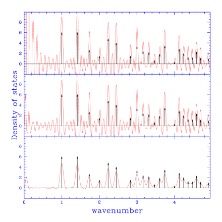
FIG. 2.: This illustrates the recovery of the known discrete spectrum in the $T^{3}$ model of size $L=2\pi$ using the method of images. Plots of $(2\pi^{2}/k^{3})~{}n^{T^{3}}(k)$ in the three panels show the density of states obtained at different stages of our method. The left panels implement the limiting procedure of eq.(14), varying the number of shells $N$ of images that are summed. Images up to $N=9$ layers ($=19^{3}$ images ) are used. The right panels use the radial limiting procedure of eq.(36), with a cut-off radius $r_{*}$ that we use for CH spaces; here, $r_{*}=9L$, with only $3071$ nearest images used. The vertical arrows mark the location of the discrete eigenvalues with the height proportional to the occupation number. The topmost panel shows the unregularized spectrum. Note the huge spurious contribution from the $k=0$ mode below the fundamental mode at $k=1$. The middle panel shows the result of regularization. At this stage most of the spurious power is removed. The result of Cesaro resummation shown in the bottom panel demonstrates that our method finally recovers a smoothed power spectrum with negligible spurious long wavelength power. Note that the radial limiting procedure does better in terms of removing spurious power at low $k$.

It is important to realize that at a given partial image sum the correlation function is obtained to far better accuracy than the power spectrum. The correlation function is a $k$-space integral over the power spectrum and is accurately reproduced as long as power is sufficiently peaked around the correct eigenvalues and there is not much overlap between the adjacent peaks. The partial image sum generates a spectrum which can be approximated as the true spectrum convolved with a smearing function, $W((k-k_{i})^{2}/(\Delta k)_{s}^{2})$, around the true eigenvalues. Here $(\Delta k)_{s}$ quantifies the width of the smoothing. In a compact space no two points are physically separated by more than the diameter of the space. Hence, to get a reasonably accurate estimation of the correlation function, it is sufficient to ensure that $R_{s}\sim 1/(\Delta k)_{s}$ is larger than the diameter of the space. In the case of the simple $T^{3}$ model, in the Gaussian approximation to the smearing function $W$, the method of images with $N$ layers gives $R_{s}=(2/3)d_{T}\sqrt{N(N+1)}$ where $d_{T}=L\sqrt{3}/2$ is the diameter of the simple $T^{3}$. Hence, the second layer ($N=2$) approximation satisfies the $R_{s}>d_{T}$ condition by a comfortable margin, and even the first layer comes fairly close.

The above estimate of the spread in the peaks around eigenvalues is based solely on the regularized spectrum done with summation in layers up to $N$ layers. We also carry out a Cesaro resummation to remove remaining spurious low $k$ power. The resummation procedure effectively averages the cumulative results at each layer. It is not difficult to see that this reduces the amplitude of the peak by a factor of two and broadens the spectrum by the same factor. Thus to reach the same spectral resolution after Cesaro resummation one need to go to $N_{c}\approx 2N$ layers. We prefer to implement the radial limiting procedure, which is simpler and does better at the resummation stage in suppressing residual low $k$ power. Equating the number of images of the radial limiting procedure to that in $N_{c}$ layers implies choosing $r_{*}/L\approx(3/4\pi)^{1\over 3}(2N_{c}+1)$. Hence, for the resummed spectrum obtained with the radial limiting procedure, the comfortable margin of $N=2$ (which translates to $N_{c}=4$) estimated above for obtaining accurate correlation functions translates to $r_{*}\approx 5.6L$. In the second panel of Figure 3, we show the spectrum recovered at $r_{*}=5.5L$.

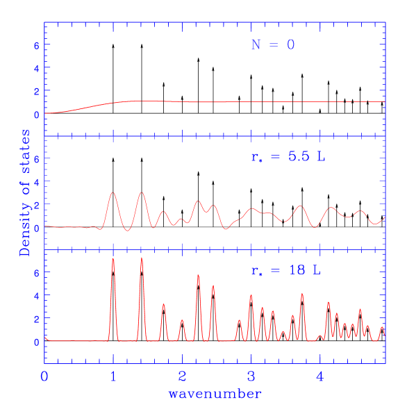
FIG. 3.: The recovery of the known discrete spectrum $(2\pi^{2}/k^{3})~{}n^{T^{3}}(k)$ in the $T^{3}$ model of size $L=2\pi$ using the method of images. The top panel shows the regularized spectrum obtained at the lowest level approximation ($N=0$, nearest image): only the low $k$ cutoff is recovered. The second panel is the spectrum recovered after summing images up to a distance of $r_{*}=5.5L$, a level of approximation which should (and does) recover the correlation function quite well, although the spectrum is coarse. The bottom panel demonstrates the convergence of the regularized method of images: with a large enough number of images, the spectrum is also recovered with precision. In the lower two panels, Cesaro resummation has been carried out on the regularized spectrum.

Another important remark is in order. In application to CMB, the positions of points ${\bf x},{\bf x}^{\prime}$, between which the correlation function is to be calculated, are given by the length and directions of the photon path from the observer, i.e., correspond to the coordinates on the universal cover ${\cal M}^{u}$. In the method of images, the value of $\xi^{c}_{\Phi}({\bf x},{\bf x}^{\prime})$ for the pairs of points belonging to separate domains is found by symmetric replication of the correlation value computed after ${\bf x}^{\prime}$ is mapped back into the Dirichlet domain around ${\bf x}$. Thus, the method of images applied to the correlation function preserves at all levels of approximation the exact periodicity of the $\xi^{c}_{\Phi}({\bf x},{\bf x}^{\prime})$ viewed as being defined on the universal cover. This periodicity is the major distinction between $\xi^{c}_{\Phi}({\bf x},{\bf x}^{\prime})$ and the correlation function $\xi^{u}_{\Phi}({\bf x},{\bf x}^{\prime})$ in the simply connected universal cover space. In contrast, a correlation function determined as the inverse transform with respect to the universal cover eigenmodes of the approximate power spectrum will fail to obey the symmetries of the compact tiling strictly. This failure is greater the cruder the level of approximation used for computing the power spectrum.

The success at reconstructing the correlation function by the method of images with even just a few layers of summation is demonstrated in Figure 4. In accordance with the estimate of the convergence of the method, summation over 5 layers (N=5.5) and above produces a correlation function almost indistinguishable from the exact result. $N=3.5$ is already very good and even $N=1.5$ is an adequate approximation of the result. Even from the very beginning, with only the nearest image used, the method of images correctly catches the qualitative behavior of the correlation function in the compact space, which is dramatically different from the corresponding correlation function in non-compact flat space.

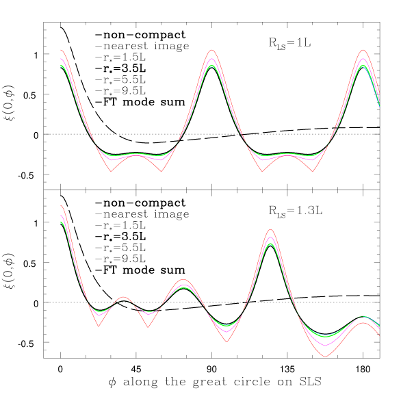
FIG. 4.: Correlation function in $T^{3}$, calculated by the method of images with successively increasing number of images, is compared with the exact summation of eigenmodes of the Laplacian via Fourier transformation. Anticipating application to the CMB, we plot the correlation values between the points along the great circle of radius $R_{\sc ls}$ and one fixed point on the circle at $(R_{\sc ls},0,0)$. The orientation of Cartesian coordinates coincides with directions of periodicity of the torus, so $\phi$ is the polar angle. Monopole and dipole contributions along the circles (i.e., different on each circle) are subtracted. The results are shown for two values of $R_{\sc ls}$: The first case when $R_{\sc ls}=1$ is a very symmetric one where points at $0,90,180,\ldots$ degrees on the great circle are exact images of the point at the origin. The second case is a more general one. Labels mark the curves from top to bottom at zero lag, $\phi=0$.

V Compact Hyperbolic spaces

A Correlation function on ${\cal H}^{3}$

The local isotropy and homogeneity of ${\cal H}^{3}$ implies $\xi^{u}_{\Phi}({\bf x},{\bf x}^{\prime})$ depends only on the proper distance, $r\equiv d({\bf x},{\bf x^{\prime}})$, between the points ${\bf x}$ and ${\bf x^{\prime}}$. The eigenfunctions on the universal cover are of course well known for all homogeneous and isotropic models [31]. Consequently $\xi^{u}_{\Phi}({\bf x},{\bf x}^{\prime})$ can be obtained through eq. (2). The role of $\xi^{u}_{\Phi}(r)$ in the compact space calculation is to impose the desired power spectrum of $\Phi$. In line with the application for which we developed our method, we now specialize to the scalar field $\Phi$ being the one describing cosmological gravitational potential fluctuations.

The initial power spectrum of the gravitational potential $P_{\Phi}(k)$ is believed to be dictated by an early universe scenario for the generation of primordial perturbations. We assume that the initial perturbations are generated by quantum vacuum fluctuations during inflation. This leads to

$$\xi^{u}_{\Phi}({\bf x},{\bf x}^{\prime})\equiv\xi^{u}_{\Phi}(r)=\int_{0}^{\infty}\frac{d\beta~{}\beta}{(\beta^{2}+1)}~{}\frac{\sin(\beta r)}{\beta\sinh r}~{}~{}{\cal P}_{\Phi}(\beta)\,,$$ (35)

where $\beta\equiv\sqrt{(kd_{c})^{2}-1}$, ${\cal P}_{\Phi}(\beta)\equiv\beta(\beta^{2}+1)P_{\Phi}(k)/(2\pi^{2})$ and, as before, $r$ is in units of $d_{c}$. In the simplest inflation models, the power per logarithmic interval of $k$, i.e., ${\cal P}_{\Phi}$, is approximately constant in the “subcurvature sector”, defined by $kd_{c}>1$. This is the generalization of the Harrison-Zeldovich spectrum in spatially flat models to hyperbolic spaces [32, 33]. In appendix A, we outline a simplified calculation of the initial inflationary perturbation spectra ${\cal P}_{\Phi}$ in hyperbolic geometry and derive a broader class of “tilted” spectra. Sub-horizon vacuum fluctuations during inflation are not expected to generate supercurvature modes, those with $kd_{c}<1$, which is why they are not included in eq.(35). Indeed, since $H^{2}>1/(ad_{c})^{2}$, for modes with $kd_{c}<1$ we always have $k/(aH)<1$ so inflation by itself does not provide a causal mechanism for their excitation. Moreover, the lowest non-zero eigenvalue, $k_{1}>0$ in compact spaces provides an infra-red cutoff in the spectrum which can be large enough in many CH spaces to exclude the supercurvature sector entirely ($k_{1}d_{c}>1$). (See $\S$V C.) Even if the space does support supercurvature modes, some physical mechanism needs to be invoked to excite them, e.g., as a byproduct of the creation of the compact space itself, but which could be accompanied by complex non-perturbative structure as well. To have quantitative predictions for $P_{\Phi}(k)$ would require addressing this possibility in a full quantum cosmological context. For a recent discussion of the creation of hyperbolic universes within a quantum cosmological framework see [34].

B Numerical implementation of the method of images

Equation (13) encodes the basic formula for calculating the correlation function using the method of images. For a numerical estimate, a limiting procedure such as eq. (14) has to be used. In this form, the regularization term involves integrating $\xi^{u}_{\Phi}({\bf x},{\bf x}^{\prime})$ over a Dirichlet domain. Such terms can be numerically computed given the discrete group of motion, $\Gamma$, but it is usually cumbersome since the Dirichlet domains of CH spaces have complicated shapes which vary depending on the basepoint.

A more effective and simpler radial limiting procedure in implementing the regularized method of images is to explicitly sum images up to a radius $r_{*}$ and regularize by subtracting the integral $\xi^{u}_{\Phi}(r)$ over a spherical ball of finite radius $r_{*}$:

$$\xi^{c}_{\Phi}({\bf x},{\bf x}^{\prime})=\lim_{r_{*}\to\infty}\left[\sum_{r_{j}<r_{*}}\xi^{u}_{\Phi}(r_{j})-\frac{4\pi}{V_{\!\cal M}}\int_{0}^{r_{*}}dr~{}\sinh^{2}r~{}\xi^{u}_{\Phi}(r)\right],~{}~{}~{}~{}r_{j}=d({\bf x},\gamma_{j}{\bf x}^{\prime})\leq r_{j+1}\,.$$ (36)

The volume element in the integral is the one for ${\cal H}^{3}$. We have shown for the flat torus that this scheme works better numerically than formal regularization which subtracts integrals over Dirichlet domains.

The plot on the left in Figure 5 illustrates the steps involved in implementing the regularized method of images. The value of $\xi^{c}_{\Phi}$ as a function of $r_{*}$ has some residual jitter, which arises because of the boundary effects due to the sharp “top-hat”averaging over a spherical ball chosen for the counterterm in eq.(36). This can be smoothed out by resummation techniques [35]. We use Cesaro resummation for this purpose.

In hyperbolic spaces, the number of images within a radius $r_{*}$ grows exponentially for $r_{*}/d_{c}>1$ and it is not numerically feasible to extend direct summation to large values of $r_{*}/d_{c}$. The presence of the counterterm, however, besides regularizing, significantly improves convergence. This can be intuitively understood as follows: $\xi^{u}_{\Phi}(r_{j})$ represents a sampling of a smooth function at discrete points $r_{j}$. In a distant radial interval $[r,r+dr],~{}r\gg R_{>},~{}dr\sim R_{>}$, there are approximately $(4\pi/V_{\!\cal M})~{}\sinh^{2}r~{}dr$ images. The sum, $\sum_{r_{j}}\xi^{u}_{\Phi}(r_{j})$, within this interval is similar to the (Monte-Carlo type) estimation of the integral, therefore one may approximate the sum over all distant images beyond a radius $r_{*}$ by an integral to obtain

$$\tilde{\xi}^{c}_{\Phi}({\bf x},{\bf x}^{\prime})=\sum_{r_{j}<r_{*}}\xi^{u}_{\Phi}(r_{j})+\frac{4\pi}{V_{\!\cal M}}\int_{r_{*}}^{\infty}dr~{}\sinh^{2}r~{}\xi^{u}_{\Phi}(r)\,.$$ (37)

The tilde on $\xi^{c}_{\Phi}({\bf x},{\bf x}^{\prime})$ denotes the fact that it is approximate and unregularized. Subtracting the integral $(4\pi/V_{\!\cal M})\int_{0}^{\infty}dr~{}\sinh^{2}r~{}\xi^{u}_{\Phi}(r)$ as dictated by the regularization eq.(13), we recover the finite $r_{*}$ term of the limiting sequence in eq.(36). This demonstrates that even at a finite $r_{*}$, in addition to the explicit sum over images with $r_{j}<r_{*}$, the expression for $\xi^{c}_{\Phi}$ in eq.(36) contains the gross contribution from all distant images with $r_{j}>r_{*}$. Numerically we have found it suffices to evaluate the above expression up to $r_{*}$ about $4$ to $5$ times the domain size $R_{>}$ to obtain a convergent result for $\xi^{c}_{\Phi}({\bf x},{\bf x}^{\prime})$.

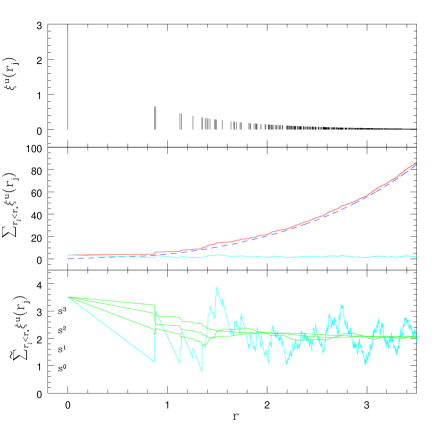
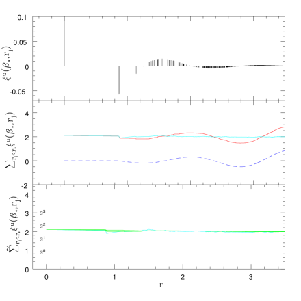
FIG. 5.: The two plots illustrate the regularization of the correlation functions with and without an infrared cut-off at $\beta_{*}>0$. The example shown is the correlation function at zero-point separation at some point on the CH manifold m004(-5,1). The plot on the left corresponds to $\xi^{c}_{\Phi}({\bf x},{\bf x}^{\prime})$ where there is no $\beta$ cut-off. The topmost panel shows the sampled values of $\xi^{u}_{\Phi}(r)$ which contribute to the sum over images. The upper solid curve in the middle panel shows the divergent cumulative build up of the partial sum over images with successive addition of distant images. The dashed curve is the regularizing counterterm required to remove the zero-mode contribution and the lower solid curve is the cumulative value of the regularized partial sum $\tilde{\xi}^{c}_{\Phi}({\bf x},{\bf x}^{\prime})$, which fluctuates around the true value once a sufficient number of images have been added. In the bottom panel this residual jitter ($s^{0}$) in the estimate of the correlation is removed by Cesaro resummation. The sequence of lines, $s^{1},s^{2}$ and $s^{3}$ shows the result of applying first, second and third order Cesaro resummation. The accuracy at the second order is usually sufficient. The plot on the right is analogous to the left but for the auxiliary correlation function $\xi^{c}_{\Phi}(\beta_{*},{\bf x},{\bf x}^{\prime})$ with an infrared cut-off at $\beta_{*}=4.0$ below the first eigenvalue in the CH space. In contrast to the left panels, the cumulative sum over images is oscillatory which is more easily regularized, leading to much smaller residual jitter around the true value.

Eq. (37) provides the simplest interpretation of our regularization procedure as an integral approximation to the total contribution of all distant images outside the region over which direct summation has been carried out. However, this interpretation may not be obvious in all cases. In fact, for the spectrum ${\cal P}(\beta)\equiv\mathrm{const}$ that we use here, the correlation function on the universal cover ${\cal H}^{3}$ is given in terms of the hyperbolic sine and cosine integral functions, ${\rm Shi}(r)$ and ${\rm Chi}(r)$, respectively, by

$$\xi^{u}_{\Phi}(r)={\rm Chi}(r)-\coth(r)\,{\rm Shi}(r)\,.$$ (38)

This is positive definite and does not fall off fast enough with $r$ for its volume integral to converge. As a result, the integral in eq.(37) is not defined and the step from eq.(36) to eq.(37) is nontrivial, involving the regularization of an infinity which can be traced to the $\beta=0$ mode. To reinstate the intuitive interpretation in this case, we first show that it is valid for an auxiliary correlation function, $\xi^{u}_{\Phi}(\beta_{*},r)$, which has an explicit infrared cutoff at $\beta_{*}>0$. The auxiliary correlation function

$$\xi^{u}_{\Phi}(\beta_{*},r) = \int_{\beta_{*}}^{\infty}\frac{d\beta~{}\beta}{(\beta^{2}+1)}~{}\frac{\sin(\beta r)}{\beta\sinh r}~{}~{}{\cal P}(\beta)$$ (39)

$$= -{\rm Re}\left\{\left[{\rm Ci}\left((i-\beta_{*})r\right)+{\rm Ci}\left((i+\beta_{*})r\right)\right]/2+i\left[{\rm Si}\left((i+\beta_{*})r\right)+{\rm Si}\left((i-\beta_{*})r\right)\right]/2\coth r\right\},$$ (40)

where ${\rm Si}(r)$ and ${\rm Ci}(r)$ are the sine and cosine integral functions, respectively. This function, $\xi^{u}_{\Phi}(\beta_{*},r)$, is no longer positive definite and its volume integral, although an improper integral, can be shown to be zero.

The contribution to $\xi^{c}_{\Phi}(\beta_{*},{\bf x},{\bf x}^{\prime})$ of the distant images with $R\gg\beta_{*}^{-1}$ can now be evaluated explicitly:

$$4\pi\int_{R}^{\infty}dr~{}\sinh^{2}r~{}\xi^{u}_{\Phi}(\beta_{*},r)\stackrel{{\scriptstyle R\gg\beta_{*}^{-1}}}{{\longrightarrow}}-\frac{4\pi}{V_{D}k_{*}^{3}}\sin\left(\beta_{*}R+\sin^{-1}(k_{*}^{-1})\right)~{}\frac{\sinh R}{R}\,.$$ (41)

This is purely oscillatory with a zero mean. The plot on the right in Figure 5 shows that these oscillations of the regularization term precisely cancel out the oscillations (with growing amplitude) of the image sum, with no net effect on the limiting value of $\xi^{c}_{\Phi}(\beta_{*},{\bf x},{\bf x}^{\prime})$.

Having established that eq. (37) makes sense for $\xi^{c}_{\Phi}(\beta_{*},{\bf x},{\bf x}^{\prime})$, where $\beta_{*}>0$, the interpretation may now easily be extended to $\xi^{c}_{\Phi}({\bf x},{\bf x}^{\prime})$ by simply noting that given $0<\beta_{*}\ll\beta_{1}$, where $\beta_{1}$ is the wavenumber corresponding to the first eigenvalue of the Laplacian in the CH space, the method of images applied to the auxiliary $\xi^{u}_{\Phi}(\beta_{*},r)$ and $\xi^{u}_{\Phi}({\bf x},{\bf x}^{\prime})$ must converge to the same value. This result is demonstrated in Figure 6.

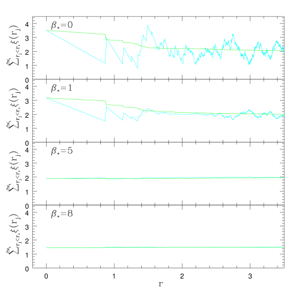
FIG. 6.: The analog of the bottom panels of Figure 5 for three values of the cut-off $\beta_{*}$. The more jagged curve is a regularized sequence of partial sums and the smoother curve is the result of a third order Cesaro resummation on the regularized result. The effectiveness of regularization is enhanced (reflected in the smaller amplitude of jitter) as one increases the value of $\beta_{*}$ by directly cutting out more of the zero-mode contamination. The computation is robust and converges to the correct value as long as $\beta_{*}\ll\beta_{1}$. For the CH manifold m004(-5,1) used in this figure, we estimate $\beta_{1}\mathrel{\hbox to0.0pt{\lower 3.0pt\hbox{$\mathchar 536\relax$}\hss}\raise 2.0pt\hbox{$\mathchar 318\relax$}}5$ (see Figure 7). In the top three cases, $\beta_{*}\leq 5$, and the computed correlation converges to $\xi^{c}(0)=2$ with high accuracy, independent of $\beta_{*}$. When $\beta_{*}>\beta_{1}$, the value of $\xi^{c}(0)$ is underestimated, as is seen in the bottom most panel where $\beta_{*}=8$.

C Power spectrum

In this section, we present our results on the power spectrum of CH manifolds obtained by applying the method of images to the density of states kernel $n^{u}(k,{\bf x},{\bf x}^{\prime})$ discussed in $\S$III B. We emphasize that evaluating the density of states numerically in CH spaces is not our primary goal. What we present is a rough estimate of the power spectra in CH spaces that can be readily obtained as a ‘byproduct’ of our primary goal of computing correlation functions in CH spaces.

Indeed, in the formalism of images, the singular delta-functions in $n^{c}(k)$ (see eq (19)) are recovered, in principle, by the precise cancellation of the smooth contributions from all images. The volume of a sphere in ${\cal H}^{3}$, and consequently the number of images (of the Dirichlet domain of a CH space on the universal cover), grows exponentially with radius beyond $r\sim d_{c}$. This is the primary constraint on the success of applying the method of images to the density of states.

Our approximation for computing the CH space correlation function includes the gross integral estimate of the impact of distant images which results in a spread-out convolved density of states distribution. Increasing $r_{*}$ progressively sharpens spectral profiles near the true positions of the discrete eigenvalues [36]. Figure 7 shows a sample $n^{c}(k,{\bf x},{\bf x})$ for some of the CH manifolds at two random positions ${\bf x}$ in the first two columns. The third column shows the smoothed out estimation of the actual density of states, $n^{c}(k)$, for the CH manifolds that one can obtain by averaging $n^{c}(k,{\bf x},{\bf x})$ over $\sim 10^{3}$ points on the manifold.

There is a definite signature of strong suppression of power at small $\beta$ in all the cases that we have explored. This is qualitatively similar to the infrared cutoff known for the compact manifolds with flat and spherical topology. Quantitatively, the break appears around $k\sim{\cal O}\left(d_{\!\cal M}^{-1}\right)$, consistent with the intuitive expectations.

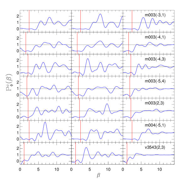
FIG. 7.: The density of states exhibits suppression of long-wave power if the Universe has compact topology. Each row corresponds to one compact hyperbolic space, indicated by the label in the last column. Left and middle columns show $n^{c}(k,{\bf x,x})/k^{3}$ computed with the method of images at two randomly selected points ${\bf x}$. The last column shows the spatial averaged $n^{c}(k)/k^{3}$ obtained by Monte-Carlo integration of $n^{c}(k,{\bf x,x})/k^{3}$ over the Dirichlet domain. The normalization is chosen such that the functions are equal to unity for the topologically trivial infinite open Universe. Vertical lines illustrate naive estimation of the cutoff at $k\sim\pi/d_{\cal M}$ which holds surprisingly well for the cases checked. The first 6 examples of the CH space have about the same value of $d_{\cal M}$. These spaces have volumes $V/d_{c}^{3}$ around unity. The sixth space is m004(-5,1), the “small”space used in many of our examples. The seventh space is v3543(2,3), with volume $V_{\!\cal M}/d_{c}^{3}=6.45$, used as an example of a “large”space in this paper.

An infra-red cutoff at the lowest non-zero eigenvalue, $k_{1}>0$, exists for all compact spaces. Cheeger’s inequality [37] provides a lower bound on $k_{1}^{2}$ for a compact Riemannian manifold, $M$:

$$k_{1}\geq\frac{h_{C}}{2},~{}~{}~{}~{}h_{C}=\inf_{S}~{}\frac{A(S)}{min\{V(M_{1}),V(M_{2})\}}\,,$$ (42)

where the infimum is taken over all possible surfaces, $S$, that partition the space, $M$, into two subspaces, $M_{1}$ and $M_{2}$, i.e., $M=M_{1}\cup M_{2}$ and $S=\partial M_{1}=\partial M_{2}$ ($S$ is the boundary of $M_{1}$ and $M_{2}$). Cheeger’s isoperimetric constant $h_{C}$ depends more on the geometry than the topology of the space, with small values of $h_{C}$ achieved for spaces having a “dumbbell-like”structure – a thin bottleneck which allows a partition of the space into two large volumes by a small-area surface [37, 38]. Regular shaped compact spaces do not allow eigenvalues which are too small. For example, the Cheeger limit for all flat $T^{3}$ manifolds is $k_{1}\geq 2/L$, where $L$ is the longest side of the torus. Although the direct estimation of $h_{C}$ is not simple, for any compact space ${\cal M}$ with curvature bounded from below there exists a lower bound on $h_{C}$ in terms of the diameter of ${\cal M}$ [39, 29]; for a 3-dimensional CH space,

$$k_{1}\geq h_{C}/2\geq\frac{1}{d_{\!\cal M}}~{}{\left[2\int_{0}^{1/2}\!\!dt\cosh^{2}(t)\right]}^{-1}=0.92/d_{\!\cal M}.$$ (43)

This result prohibits supercurvature modes for all CH spaces with $d_{\!\cal M}<0.92\,d_{c}$.

There are other lower bounds on $k_{1}$ that exist in the literature. In terms of the diameter alone, the bound $k_{1}^{2}\geq\pi^{2}/(2d_{\!\cal M})^{2}-{\mathrm{m}ax}\{-(n-1)K,0\}$ has been derived for any compact $n$ dimensional space, with $K=0$ for flat geometry and $K=\pm d_{c}^{-2}$ for spherical and hyperbolic geometries, respectively [40]. For hyperbolic spaces, this bound is sharper than the one above for $d_{\!\cal M}\mathrel{\hbox to0.0pt{\lower 3.0pt\hbox{$\mathchar 536\relax$}\hss}\raise 2.0pt\hbox{$\mathchar 316\relax$}}0.9\,d_{c}$. There is another lower bound on $k_{1}$ in terms of the volume as well as the diameter [41]; for CH spaces $k_{1}\geq{\cal V}_{\!\cal M}/[2\pi d_{\!\cal M}(\sinh(2d_{\!\cal M}/d_{c})-2d_{\!\cal M}/d_{c})]$. This lower bound dominates in the supercurvature sector for volumes larger than $\approx 7d_{c}^{3}$.

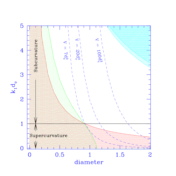
FIG. 8.: Some known bounds on the first non-zero eigenvalue in CH spaces are shown. The heavily shaded region is the lower bound in eq. (43). The lightly shaded region is the lower bound derived in [40]. The dashed lines show the lower bound which depends on volume as well for three values of the volume. The shaded regions in the top right corner define two upper bounds on $k_{1}$. The horizontally shaded region is the upper bound coming from comparison with Dirichlet eigenvalues [42]. The other region is the sharpest possible bound that can arise using the upper bound in terms of $h_{C}$ [43] and the lower bound on $h_{C}$ in eq. (43).

There are also upper bounds on $k_{1}$. The bound, $k_{1}^{2}\leq 4h_{C}/d_{c}+10h_{C}^{2}$ [43], does not allow for a firm conclusion that the space supports supercurvature modes, $k_{1}d_{c}<1$, unless $d_{\!\cal M}\geq 10.6\,d_{c}$ (using eq. (43)). Upper bounds based on comparison with the first Dirichlet eigenvalue [42] on a subdomain of ${\cal M}$ cannot impose $k_{1}d_{c}<1$, since Dirichlet eigenvalues cannot be less than $d_{c}^{-1}$.

The density of states $n^{c}(k)$ defines the eigenvalue spectrum of the Laplacian on a compact space. It is well known that there exist very strong connections between the geometry and the topology of the space and the spectral properties of the Laplacian. As discussed above, the infra-red cut off in the spectrum is broadly determined by the size (diameter) of the space and its volume.

The Weyl formula is an example of a general and powerful result connecting number of states to the topology of the compact space: for large $k$, the number of eigenvalues $N(k)\equiv\#\{j|k_{j}<k\}$ up to a given value $k$, in an $n$ dimensional compact space of volume $V_{\!\cal M}$, is given by [29]

$$N(k)\equiv\#\{j|k_{j}<k\}\approx c(n)V_{\!\cal M}k^{n}+{\cal O}(k^{(n-1)})\,,~{}~{}~{}~{}~{}~{}~{}~{}~{}c(n)=V(unit~{}ball)/(2\pi)^{n}\,.$$ (44)

The constant $c(n)$ is related to the volume within a unit sphere, set by the geometry of the space. In eq.(44), $j$ counts the eigenvalues, including multiplicity. As a corollary, the eigenvalues asymptotically can be estimated:

$$k_{j}\sim c(n)^{-1/n}(j/V_{\!\cal M})^{1/n}\ {\rm as}\ j\to\infty\,.$$ (45)

The corrections to Weyl’s asymptotic formula are ${\cal O}(k^{(n-2)+2/(n+1)})$ for flat tori and ${\cal O}(k^{(n-1)}/\ln(k^{2}))$ for manifolds with negative curvature.

Weyl’s formula also points to the dependence of the infra-red cut off on size: the smaller the space, the larger the infra-red cutoff. Eq. (45) shows that in the limit of large eigenvalues the typical spacing between distinct eigenvalues is given by the inverse of its linear size. These are familiar and intuitive facts in Euclidean compact spaces such as the simple tori. Weyl’s formula encourages the view that these broad features in the spectra of the compact manifolds transcend the geometry. Another important point of Weyl’s formula relevant for our work is that the cumulative number of eigenstates asymptotically depends only on the volume of the manifold and not on its exact topology. Thus, the gross properties of the spectrum are shared by spaces with comparable volumes, and quantities which are fairly democratically weighted integrals of the power spectrum can be expected to be similar.

VI Correlations in Compact Hyperbolic spaces

As a prelude to our computation of CMB temperature anisotropy correlations for CH spaces in [16], we focus our attention in this section on the $\Phi$-correlation function $\xi^{c}_{\Phi}({\bf x},{\bf x}^{\prime})$ between points ${\bf x}$ and ${\bf x}^{\prime}$ that belong to a $2$-sphere around the origin in ${\cal M}^{u}$ — i.e., there exist discrete motions $\gamma,\gamma^{\prime}\in\Gamma$ such that the points $\gamma{\bf x},\gamma^{\prime}{\bf x}^{\prime}\in{\cal M}^{u}$ are equidistant from the origin.

Correlation functions of this kind arise in evaluating large angle CMB anisotropies associated with the gravitational potential on the sphere of last scattering (SLS) – the Naive Sachs-Wolfe (NSW) effect. (The radius of the SLS, $R_{\sc LS}\approx 2\tanh^{-1}\sqrt{1-\Omega_{0}}$, is related to the density parameter, $\Omega_{0}$.) The angular correlation $C(\hat{q},\hat{q}^{\prime})$ between the NSW CMB anisotropy in two directions $\hat{q}$ and $\hat{q}^{\prime}$ is given by

$$C(\hat{q},\hat{q}^{\prime})\equiv\left\langle\frac{\Delta T}{T}(\hat{q})\frac{\Delta T}{T}(\hat{q}^{\prime})\right\rangle {}=\frac{1}{9}\langle\Phi(\hat{q}{\chi_{\!{}_{\rm H}}},\tau_{\sc ls})\Phi(\hat{q}^{\prime}{\chi_{\!{}_{\rm H}}},\tau_{\sc ls})\rangle~{}.$$ (46)

In simply connected universes, $C(\hat{q},\hat{q}^{\prime})\equiv C(\hat{q}\cdot\hat{q}^{\prime})$ is statistically isotropic. In contrast, for all compact universe models with Euclidean or Hyperbolic geometry, $C(\hat{q},\hat{q}^{\prime})$ is statistically anisotropic. The breakdown of isotropy leads to characteristic patterns in the predicted CMB anisotropy determined by the shape of the Dirichlet domain around the observer. Moreover, except for the simple flat torus, the global inhomogeneity implies that the variance $C(\hat{q},\hat{q})$ varies with direction $\hat{q}$. This implies that the CMB sky would be a realization of an inhomogeneous field that would have characteristic patterns of ‘loud’ and ‘quiet’ regions. These two effects constitute two aspects of the signature of a compact universe.

There are three distinct regimes for the correlation patterns on the sky in a compact space. For $R_{\sc LS}>R_{>}$, the patterns are mainly dominated by the mapping of the SLS into the compact space. The NSW-CMB patterns are characterized by spikes of positive correlation when the neighborhood of one point on the SLS is multiply-imaged on the SLS. For $R_{\sc LS}\ll R_{<}$, i.e., the SLS is well within a single domain, the compact space is indistinguishable from a simply-connected space with the same geometry. In the intermediate $R_{<}\mathrel{\hbox to0.0pt{\lower 3.0pt\hbox{$\mathchar 536\relax$}\hss}\raise 2.0pt\hbox{$\mathchar 316\relax$}}R_{\sc LS}\mathrel{\hbox to0.0pt{\lower 3.0pt\hbox{$\mathchar 536\relax$}\hss}\raise 2.0pt\hbox{$\mathchar 316\relax$}}R_{>}$ regime, there is very little multiple imaging; nevertheless, the SLS is large enough to feel the compactness of the space. Typically the correlation pattern retains the structure of correlation in the simply connected space, but is significantly deformed.

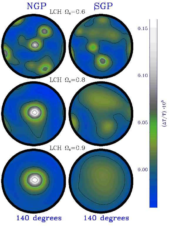
FIG. 9.: Typical angular correlation patterns $C(\hat{q}_{0},\hat{q})$ of the naive (or surface) Sachs-Wolfe effect on CMB anisotropy around a fixed direction $\hat{q}_{0}$ in the L(arge)CH model are shown as full-sky maps at the angular resolution of $5.2^{\circ}\times 5.2^{\circ}$ pixels. The full-sky maps are plotted as pairs of $180^{\circ}$ diameter hemispherical caps, one centered on the South Galactic Pole (SGP) and one on the North (NGP). $\hat{q}_{0}$ points to the NGP. In a simply connected universe, the contours of equal correlation would be concentric circles around $\hat{q}_{0}$, due to the global isotropy. The three values of $\Omega_{0}$ are representative of the three regimes. In the top panel, the radius of the SLS, $R_{\sc LS}$, is greater than $R_{>}$ and one sees multiple imaging. In the second, with $R_{<}<R_{\sc LS}<R_{>}$, there are significant distortions but no multiple imaging. The bottom panel has $R_{<}\ll R_{\sc LS}$, and no observable correlation signatures of compactness. In all the maps, the dipole component of the correlation function has been subtracted. The maps have also been smoothed by a $1.66^{\circ}$ Gaussian filter.

Figure 9 illustrates the typical correlation pattern $C({\hat{q}_{0}},{\hat{q}})$ in the large CH model v3543(5,1) around a fixed direction, ${\hat{q}_{0}}$, which we chose to correspond to a fiducial “North Galactic Pole”(NGP). Of course, the global anisotropy implies that this pattern will differ for different choices of ${\hat{q}_{0}}$. At $\Omega_{0}=0.6$, the SLS is larger ($R_{\sc ls}=1.44$) than the domain ($R_{>}=1.32$), and spikes of enhanced correlation are seen with widely separated directions when the fixed point on the sphere, or points physically close to it, are multiply imaged on the SLS. At $\Omega_{0}=0.8$, the SLS is smaller ($R_{<}<R_{\sc ls}=0.93<R_{>}$) and high correlation spikes due to multiple imaging are absent. Nevertheless, the compactness of the space is evident in the distorted contours around ${\hat{q}_{0}}$. At $\Omega_{0}=0.9$, the SLS is completely contained within the domain, and the correlation around the NGP is circularly symmetric. As expected, in this regime the compactness of the space on scales much larger than the horizon has very little observational signal. The contours show only slight, observationally insignificant, distortions.

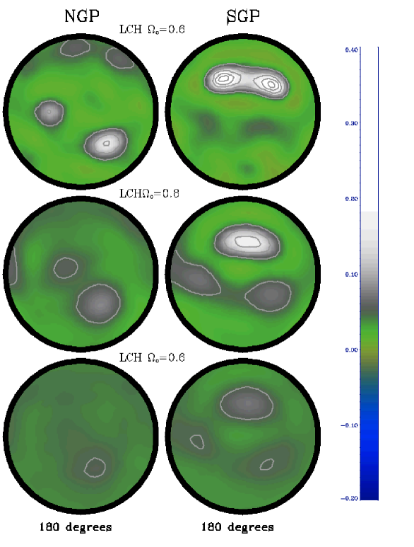
FIG. 10.: The variations in the variance $C(\hat{q},\hat{q})$ of a scalar field on three concentric spheres around the same basepoint. The radius of the spheres correspond to $R_{\sc LS}$ at the values of the density parameter $\Omega_{0}$ shown. The variance is shown in full-sky maps plotted as pairs of $180^{\circ}$ diameter hemispherical caps, one centered on the South Galactic Pole (SGP) and one on the North (NGP). In addition to the cobe–dmr beam smoothing, the maps have been smoothed by a $1.66^{\circ}$ Gaussian filter. The loud feature seen at $\Omega_{0}=0.8$ ($R_{<}<R_{\sc LS}<R_{>}$) corresponds to $\approx 100\%$ excess in the variance over its mean. At $\Omega_{0}=0.6$, the spot is multiply-imaged since the sphere is larger than the domain $R_{\sc LS}>R_{>}$. At $\Omega_{0}=0.9$ there is very little variation over the small sphere $R_{\sc LS}\ll R_{<}$.

Figure 10 plots the variance in the NSW-CMB temperature, $C(\hat{q},\hat{q})$, in the large CH model v3543(5,1) for three values of $\Omega_{0}$. The first two maps show a significant loud feature at $\Omega_{0}=0.6$ and $\Omega_{0}=0.8$, corresponding to the radii $R_{\sc LS}=1.44$ and $R_{\sc LS}=0.93$, respectively. The loud spot on the sphere at $\Omega_{0}=0.8$ is within the domain. At $\Omega_{0}=0.6$, the sphere is larger than the domain ($R_{>}=1.32$), and the loud spot is multiply imaged on the sky. The third map has $\Omega_{0}=0.9$, corresponding to a sphere of radius $R_{\sc LS}=0.63$, which is significantly smaller than the inradius, $R_{<}=0.89$. The variance does not show much variation over this small sphere around the observer.

The CMB anisotropy has contributions other than the NSW term in eq. (46). In particular, there is an integrated Sachs-Wolfe contribution (ISW), with the integration along the line of sight from the SLS to the observer. The NSW term dominates when the density parameter $\Omega_{0}$ is close to unity. When the ISW contribution is important, it significantly modifies the correlation patterns, as discussed in our companion paper [16].

VII Discussion

The computation of the angular correlation function of the CMB anisotropy requires machinery to compute spatial correlation functions on equal-time spatial 3-hypersurfaces. We have presented a general method of calculating these for multiply connected spatial sections which evades the task of eigenmode decomposition. This is particularly useful when considering compact hyperbolic models of the universe for which rather little is known about the spectrum of the Laplacian, and eigenmode decomposition is known to be difficult to obtain.

We summarize here the basic knowledge we require of a given manifold to use our method and the steps to be followed to obtain a given accuracy level for the correlation functions.

For the selected compact model ${\cal M}={\cal M}^{u}/\Gamma$ of interest, we must be able to construct the tiling of the universal cover ${\cal M}^{u}$ from the generators of group $\Gamma$ (§ II) up to some distance $r_{*}$ from the origin, which will be determined by the required level of accuracy. This is in itself a daunting mathematical task, but, fortunately, for many thousand compact hyperbolic models, the Snappea package [28] gives enough information for us to carry out this step.

Given the tiling, we perform our correlation function calculation in a sequence of radial shells of size $r$, testing whether a stopping criterion based on a desired level of convergence in the regularized summation over images (§ V B) is satisfied; if so, this defines $r_{*}$. It may be that the required $r_{*}$ is beyond the computational power at hand. For the correlation function calculations of interest for the CMB problem in the compact hyperbolic spaces we have tried, $10^{5}$ images are computationally very feasible (less than a day on a 433 MHz alpha workstation). This allows us to go out to $r_{*}\approx 5d_{\!\cal M}$, more than adequate for convergence.

It may be for manifolds with very many faces, the number of images required to converge could be prohibitive. Even if this is so, we obtain useful results out to the radius we can achieve because at each shell $r$ the symmetries of the manifold are preserved in the correlation function. Indeed even the nearest few shells of images are enough for a qualitatively correct result on the basic pattern of correlations, which is also quantitatively not too bad. We showed explicitly for the flat torus (§ IV) that the correlation function is well determined as long as the density of states calculated for that number of shells has the power in each discrete mode localized to within $\Delta k_{i}\sim 1/d_{\!\cal M}$ around the true eigenvalue $k_{i}$. Since the line of argument leading to this result is independent of the local geometry of the compact space, it applies to CH spaces as well.

Our method has the merit of avoiding explicit eigenmode decomposition. Recently progress has been reported in directly computing the low-$k$ eigenmodes of the Laplacian for selected compact hyperbolic spaces [14]. It has proved necessary to use spectral line “deblending” techniques in conjunction with these methods to get the eigenvalue spectrum accurately [15]. As we showed in § III B, we can also use the method of images to calculate the spectrum of eigenvalues, though this is more difficult than correlation function evaluation since it requires longer summations to get narrow spectral lines, as is evident from Fig. 3 and [2]. These figures immediately suggesting deblending, but at this stage, only for the torus case do we explicitly know the shapes of the broadened spectral lines obtained by sequential image addition. One of the manifolds in which the low-$k$ eigenvalues were determined by Inoue [14] is in common with those we have computed the spectrum for. We find his results agree with ours.

The goals of this paper were to provide a detailed description of our regularized method of images, demonstrate that it works extremely well, and more generally show the basic effects of compactness on the correlation function of a scalar field and the density of states of the Laplacian. The computation of large angle CMB anisotropy, the features that arise in the CMB correlation that are characteristic of compact spaces, the detailed comparison with the cobe–dmr data and the constraints that follow using large and small CH space examples are presented in the companion paper [16]. A compilation of the constraints from the all sky cobe–dmr data on a large selection of CH spaces will be presented in [45].

VIII Acknowledgements

We acknowledge the use of the SnapPea package and related material on compact hyperbolic spaces available at the public website of the Geometry center at the University of Minnesota. TS acknowledges support during the final stages of this work from NSF grant EPS-9550487 with matching support from the state of Kansas. In the course of this project we had enjoyable interactions with J. Levin, N. Cornish, D. Spergel, I. Sokolov, G. Starkman and J. Weeks.

A Inflationary perturbations in a Hyperbolic universe

It is widely accepted that the large scale structures in the present Universe grew out of small initial metric perturbations via the mechanism of gravitational instability. The inflationary epoch in the Universe provides us with a setting for the generation of fluctuations with power on large scales. Cosmological perturbations are effectively massless (light) scalar fields residing on a background FRW space-time and the large scale power is related to the infra-red behavior of the light scalar field propagator in the inflationary epoch. In this Appendix, we present a simplified calculation of the initial power spectra for open inflation (hyperbolic geometry) to place the spectrum that we use in our work within a broad class of “tilted” inflationary spectra which are “scale free” on scales much smaller than $d_{c}$ and are analogous to the well-known tilted spectra in Euclidean (flat) inflationary universe. The scope of our analysis is limited by the particular choice of the vacuum state, as discussed below.

Inflationary scenarios that lead to a simply connected hyperbolic universe generally require two stages [46]. This is because a single stage of inflation cannot provide homogeneity across the Hubble patch without inflating the local curvature in the patch to negligible values. A widely prescribed solution is to invoke a “creation stage” involving the creation of a universe with homogeneous hyperbolic spatial sections which is then followed by a sufficiently short inflationary stage (so as not to expand the curvature away) inflationary stage responsible for generating the primordial perturbations at cosmological scales. Since the second epoch of inflation cannot be long, the specifics of the first stage of creation of ${\cal H}^{3}$ spatial sections could influence the spectrum of generation of perturbations at supercurvature scales. The possible effects on the spectrum have been extensively studied in recent literature [47] in the context of open-bubble models in which the open universe resides in the interior of the bubble nucleated in the first-order phase transition from a larger inflating universe. It is doubtful, however, that the bubble mechanism can be used to produce compact hyperbolic spaces. More relevant is probably the mechanism of quantum creation of the universe “from nothing” where the topology of the created space is related to the topological properties of the instanton solution in the Euclidian section [34]. Proper quantization of the fluctuations in such a scenario is, however, still a matter for the future.

We assume that at the beginning of the second (inflationary) stage all quantum fields on the hyperbolic hypersurface are in the vacuum state and the vacuum modes in eq. (A8) are chosen by identifying the positive frequency part of the general solution to the mode evolution equation. This choice of the initial state sets the boundary of applicability for our considerations . It is important to bear in mind that, in general, the creation stage could modify the proper choice of the vacuum state and consequently the predicted spectrum eqs. (A9) and (A10).

We outline the derivation of the power spectrum for a free scalar field $\psi$ which will be appropriately identified with metric perturbations subsequently. The scalar field equation allows the spatial and temporal dependence to be separated: $\psi({\bf x},\tau)=\psi_{k}(\tau)~{}G_{\bf k}({\bf x})$. The rapid expansion of the space-time during inflation would redshift away to insignificance the number density of any pre-inflationary quanta within the first few e-folds of expansion. As a result, it is a good approximation to assume that all the fields are in their vacuum state i.e., $\psi_{k}(\tau)\equiv\psi^{(+)}_{k}(\tau)$. The vacuum expectation value of the field, $\langle\psi^{2}(\tau)\rangle$, is the coincidence limit (${\bf x}^{\prime}\to{\bf x}$) of the equal-time two-point function, $\langle\psi({\bf x}^{\prime},\tau)\psi({\bf x},\tau)\rangle$, and, hence, can be expressed as a mode-sum over the mode functions:

$$\langle\psi^{2}\rangle = \frac{1}{(2\pi)^{3}}~{}\int d^{3}k~{}\psi_{k}(\tau)~{}\psi^{*}_{k}(\tau)$$ (A1)

$$\equiv \int\frac{dk}{k}~{}\left[{k^{3}\over 2\pi^{2}}~{}\psi_{k}(\tau)~{}\psi^{*}_{k}(\tau)\right]~{}.$$ (A2)

The quantity within the square brackets represents the contribution per logarithmic $k-$ interval to the total power at a given time, $\tau$. We usually define the power spectrum by evaluating this quantity at some convenient time, $\tau_{*}$, during inflation. For instance, $\tau_{*}$ could correspond to the time during the inflationary epoch when the comoving scale, $k_{0}$, corresponding to the observed horizon was equal to the Hubble radius ($k_{0}|\tau_{1}|=k_{0}\tau_{0}$). The power spectrum, $P_{\psi}(k/k_{0})$, of the field, $\psi$, is defined to be

$$P_{\psi}(k/k_{0}) \equiv {k^{3}\over 2\pi^{2}}~{}\psi_{k}(\tau_{1})~{}\psi^{*}_{k}(\tau_{1})~{}.$$ (A3)

The present astrophysical comoving scales correspond to physical scales which were much larger than the Hubble radius at the end of inflation, hence it suffices to evaluate the amplitude of modes in the expression for the power spectrum, $P_{\psi}(k/k_{0})$, in the limit, $k\tau\to 0$.

We now compute the spectrum of initial perturbations generated in the second inflationary stage on a FRW model with ${\cal H}^{3}$ spatial sections.

The spatial modes of a scalar field on ${\cal H}^{3}$ are given by orthonormal eigenfunctions of the Laplacian in spherical coordinates:[48]

$$G_{\bf k}({\bf x})=\sum_{\ell=0}^{\infty}\sum_{m=-\ell}^{m=\ell}{\cal G}_{k}^{\ell}(r)\,\,Y_{lm}(\hat{x});~{}~{}~{}~{}~{}~{}~{}~{}{\cal G}_{k}^{\ell}(r)=\sqrt{\frac{N_{\ell}(\beta)}{\sinh r}}\,\,P^{-\ell-{\textstyle{1\over 2}}}_{-{\textstyle{1\over 2}}+i\beta}(\cosh r),$$ (A4)

$$\beta=\sqrt{|{\bf k}|^{2}-1},\,r=|{\bf x}|,~{}~{}~{}\hat{x}={\bf x}/r,~{}~{}~{}N_{\ell}(\beta)=\bigg{|}\frac{\Gamma(i\beta+\ell+1)}{\Gamma(i\beta+1)}\bigg{|}^{2}.$$ (A5)

In the above equation, the $P^{\mu}_{\nu}(x)$ are the associated Legendre functions and $\Gamma(\nu)$ is the Euler-Gamma function [49]. Owing to the isotropy of ${\cal H}^{3}$, the modes depend only $k=|{\bf k}|$. Moreover, modes with $kd_{c}\geq 1$, (i.e., , $\beta$ real and positive) form a complete orthonormal basis for free fields on ${\cal H}^{3}$, and it is convenient to use the wavenumber, $\beta$, to label these modes.

The temporal modes of the scalar field, $\psi_{\beta}$, on a hyperbolic universe, obey the equation

$$\psi_{\beta}^{\prime\prime}+2\frac{a^{\prime}}{a}\psi_{\beta}^{\prime}+\left[(\beta^{2}+1)+a^{2}m_{\rm eff}^{2}\right]\psi_{\beta}=0\,,$$ (A6)

where $m_{\rm eff}^{2}$ is the effective mass of the field and the prime denotes density derivatives with conformal time. We now consider the scalar field $\psi$ to be the fluctuations, $\delta\phi$, of the inflaton field [50, 51] and then $m_{\rm eff}^{2}$ is related to the quantities set by the evolution of the background inflaton field and the metric.

The above setting allows us to investigate quantum fluctuations during inflation in some well defined regimes. The classification here closely follows that of inflation in a flat universe. We consider the following cases:

• uniform inflationary (deSitter) expansion and $m_{\rm eff}^{2}=0$. This is the analog of standard slow-roll inflation;

• uniform inflationary expansion with a constant value of $m_{\rm eff}^{2}/H^{2}\neq 0$. This is the analog of the class of models with inverted harmonic oscillator like potentials, such as natural inflation; and

• constant equation of state during inflation. This is an abstraction of the power-law models of inflation.

In each of the above, the conditions are meant to hold in an approximate fashion over the relevant range of astrophysical scales, just as for the flat inflation analogs.

In the case of deSitter expansion, the scale factor is $a=\sinh(Ht)/H=-{\rm cosech}\tau/H$, expressed as a function of cosmic time $t$ and conformal time $\tau$. Eq. (A6) then reduces to

$$\psi_{\beta}^{\prime\prime}-2\coth\tau\,\psi_{\beta}^{\prime}+\left[(\beta^{2}+1)+(m_{\rm eff}/H)^{2}/\sinh\tau\right]\psi_{\beta}=0\,.$$ (A7)

The general solution involves associated Legendre functions $Q^{-\mu}_{-{\textstyle{1\over 2}}+i\beta}(\cosh\tau)$ and $P^{-\mu}_{-{\textstyle{1\over 2}}+i\beta}(\cosh\tau)$, multiplied by a factor $\sinh^{\frac{3}{2}}\tau$. The index $\mu=\sqrt{9/4-m^{2}_{\rm eff}/H^{2}}$. The positive frequency (vacuum mode) solution is identified with the late time asymptotics $\sim e^{-ik\tau}$. The normalized vacuum mode solution, $\psi_{\beta}^{(+)}$, is

$$\psi_{\beta}^{(+)}=H^{2}\sqrt{\frac{\Gamma({\textstyle{1\over 2}}+\mu+i\beta)}{i\Gamma({\textstyle{1\over 2}}-\mu+i\beta)}}\sinh^{2}\tau\,\,Q^{-\mu}_{-{\textstyle{1\over 2}}+i\beta}(\cosh\tau)\,,$$ (A8)

where the overall normalization is determined by normalizing the probability current, i.e., setting the Wronskian of $\psi_{\beta}^{(+)}$ equal to $ia^{-2}$.

The spectrum of initial perturbations in the inflaton field can be calculated from the vacuum mode solution through eq. (A3):

$$P_{\psi}(\beta)=\left|i\frac{\Gamma({\textstyle{1\over 2}}-\mu+i\beta)}{\Gamma({\textstyle{1\over 2}}+\mu+i\beta)}\right|^{2}\,.$$ (A9)

If $m^{2}_{\rm eff}=0$, the spectrum of initial perturbations in the inflaton field reduces to

$$P_{\psi}(\beta)=\frac{1}{\beta(\beta^{2}+1)}.$$ (A10)

This is the analog of the Harrison-Zeldovich spectrum for hyperbolic models derived in [32, 33]. In the limit $\beta\gg 1$, the spectrum goes over to the well-known flat “flicker noise”result. This is also the power spectrum which implies equal power per logarithmic interval in $|{\bf k}|$ that we use in our work on CH spaces (see $\S$V A).

The power spectrum in eq. (A9) is best numerically computed by using Lancoz’s formula for Gamma functions. Using the Stirling approximation to Gamma functions for $\beta\gg 1$, one recovers the standard tilted flat space spectrum from eq. (A9), ${\cal P}_{\Phi}\sim k^{3/2-\mu}$.

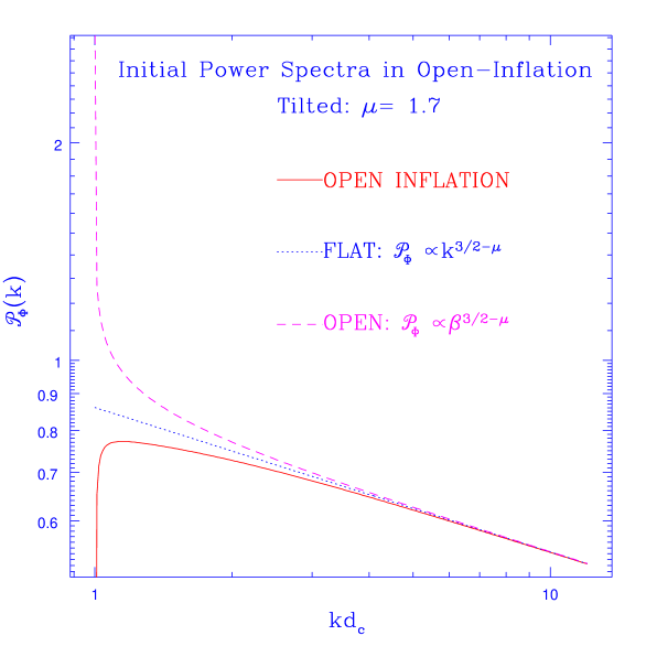
FIG. 11.: The initial power spectrum expected from inflation in a hyperbolic universe with a small tilt is shown as the solid curve (OPEN INFLATION). There is a sharp cutoff below $kd_{c}=1$ since the quantum fluctuations during inflation cannot excite supercurvature modes. The curve labeled FLAT shows the analogous tilted spectrum in a flat universe. The open inflation and the flat curves match at $kd_{c}\gg 1$. Tilted initial spectra in Hyperbolic universes have often been taken to be a power law in $kd_{c}$ or $\beta$. Although equivalent at $kd_{c}\gg 1$, these differ at small $kd_{c}$ from the inflationary prediction; the former is labeled FLAT while the latter is depicted by the dashed curve labeled OPEN. The open inflation spectrum that we use in our paper corresponds to no-tilt, $\mu=3/2$, is flat with a sharp cutoff at $kd_{c}=1$.

In the more general case of constant equation of state, $w\equiv P/\rho$, during inflation, the scale factor obeys $a=\sinh^{\alpha}(\tau/\alpha)$ where $\alpha=2/(3w+1)$. The deSitter expansion corresponds to the case $w=-1$. The eq.(A6) for the temporal modes reduces to the form

$$\psi_{\beta}^{\prime\prime}+2\coth(\tau/\alpha)\,\psi_{\beta}^{\prime}+(\beta^{2}+1)\psi_{\beta}=0~{}.$$ (A11)

The general solution of the above equation involves the same associated Legendre functions as the solution for equation (A7) with index $\mu=1/2-\alpha$, rescaled wavenumber $\tilde{\beta}^{2}=\alpha^{2}\beta^{2}=(k^{2}-1)\alpha^{2}$, rescaled time $\tilde{\tau}=\tau/\alpha$, and multiplication by a factor of $\sinh^{\mu}\tilde{\tau}$.

The positive frequency (vacuum mode) solution is identified again with the late time asymptotics $\sim e^{-ik\tilde{\tau}}$. The normalized vacuum mode solution, $\psi_{\beta}^{(+)}$, is

$$\psi_{\beta}^{(+)}=H^{2}\sqrt{\frac{\Gamma({\textstyle{1\over 2}}+\mu+i\tilde{\beta})}{i\Gamma({\textstyle{1\over 2}}-\mu+i\tilde{\beta})}}\sinh^{2}\tau\,\,Q^{-\mu}_{-{\textstyle{1\over 2}}+i\tilde{\beta}}(\cosh\tilde{\tau}).$$ (A12)

The spectrum of perturbations is of the same form as (A9) with rescaled wavenumber $\tilde{\beta}$ and $\mu=1/2-2/(3w+1)$. The spectra given by (A9) are hyperbolic universe analogs of tilted spectra generated in flat universe inflation models such as power-law inflation.

REFERENCES

- [1] J. R. Bond, D. Pogosyan and T. Souradeep, in: Proceedings of the XVIIIth Texas Symposium on Relativistic Astrophysics, ed. A. Olinto, J. Frieman, and D. N. Schramm, (World Scientific, 1997).
- [2] J. R. Bond, D. Pogosyan and T. Souradeep, Class. Quant. Grav. 15, 2671, (1998).
- [3] A. Dekel, D. Burstein and S. D. M. White, 1996, in Critical Dialogues in Cosmology, ed. N.Turok, World Scientific; D. N. Spergel, Class. Quant. Grav. 15, 2589, (1998); N. Bahcall and X. Fan, preprint (astro-ph/9804082).
- [4] G. F. R. Ellis, Gen. Rel. Grav. 2, 7,(1971).
- [5] D. D. Sokolov and V. F. Shvartsman, Zh. Eksp. Theor. Fiz. 66, 412, (1974) [JETP, 39, 196 (1974)] and references therein to the early papers on ghost searches.
- [6] M. Lachieze-Rey and J. -P. Luminet, Phys. Rep. 25, 136, (1995).
- [7] J. R. Gott, Mon. Not. R. Astr. Soc. 193, 153, (1980).
- [8] N.J. Cornish, D. N. Spergel and G. D. Starkman, Phys. Rev. Lett. 77, 215, (1996).
- [9] G. T. Horowitz and D. Marolf, J.High Energy Phys. 9807, 014, (1998).
- [10] G. Starkman, Class. Quantum Grav. 15, 2529, (1998); and other articles in the same issue: Proceedings of Topology and Cosmology, CWRU, Cleveland, Oct. 17-19, 1997 .
- [11] L. Z. Fang and H. Sato, Comm. Theor. Phys, (China) 2, 1055, (1983); H. V. Fagundes, Astrophys. J. 291, 450, (1985); ibid., Astrophys. J. 338 , 618, (1989); H. V. Fagundes and U. F. Wichoski, Astrophys. J. Lett. 322, L5, (1987).
- [12] H. V. Fagundes, Phys. Rev. Lett. 70, 1579, (1993); R. Lehoucq, M. Lachiese-Rey and J. -P. Luminet, Astron. Astrophys. 313, 339, (1996); B. F. Roukema and A. C. Edge, Mon. Not. Roy. Astron. Soc. 292, 105, (1997); B. F. Roukema and V. Blanloeil, Class. Quantum Grav. 15, 2645, (1998); J. -P. Luminet and B. F. Roukema, preprint, (astro-ph/9801364) and references therein.
- [13] R. Aurich and F. Steiner, Physica D 39, 169, (1989); R. Aurich and J. Marklof, Physica D 92, 101, (1996); R. Aurich, preprint, (astro-ph/9903032).
- [14] K. Inoue, Class. Quant. Grav. 16, 3071, (1999).
- [15] N. J. Cornish and D. Spergel, preprint, (math.DG/9906017).
- [16] J. R. Bond, D. Pogosyan, and T. Souradeep in this volume (paper-II), (1999).
- [17] A. A. Starobinsky, JETP Lett. 57, 622, (1993); A. de Oliveira Costa, G. F. Smoot and A. A. Starobinsky, Astrophys. J. 468, 457, (1996).
- [18] I. Y. Sokolov, JETP Lett. 57, 617, (1993); D. Stevens, D. Scott and J. Silk, Phys. Rev. Lett. 71, 20, (1993); A. de Oliveira Costa and G. F. Smoot, Astrophys. J. 448 477, (1995).
- [19] J. R.Bond, in Proc. of the XVIth Moriond Astrophysics Meeting, ed. F. R. Bouchet et al. ., (Editions Frontieres, France, 1997); J. R. Bond, Proc. Natl. Acad. Sci. USA, 95, 35, (1998).
- [20] J. Levin, J. D. Barrow, E. F. Bunn and J. Silk, Phys. Rev. Lett. 79, 974, (1997).
- [21] D. D. Sokoloff and A. A. Starobinski, Sov. Astron. 19, 629, (1975).
- [22] J. A. Wolf, Space of Constant Curvature (5th ed.), (Publish or Perish, Inc., 1994).
- [23] E. B. Vinberg, Geometry II – Spaces of constant curvature, (Springer-Verlag, 1993).
- [24] W. P. Thurston, The Geometry of 3-Manifolds, lecture notes, Princeton University (1979); W.P. Thurston and J. R. Weeks, Sci. Am. 251, 108, (1984).
- [25] D. Gabai, R. G. Meyerhoff and N. Thurston, preprint MSRI 1996-058, (1996).
- [26] J. R. Weeks,Ph.D. Thesis, (Princeton, 1985).
- [27] S. V. Matveev and A. T. Fomenko, Usp. Mat. Nauk. 43, 5, (1988) [ Russ. Math. Surv. 43, 3, (1988)].
- [28] J. R. Weeks, SnapPea: A computer program for creating and studying hyperbolic 3-manifolds, Univ. of Minnesota Geometry Center (freely available at http://www.geom.umn.edu).
- [29] I. Chavel, Eigenvalues in Riemannian geometry, (Academic Press, 1984).
- [30] G. Starkman, Class. Quantum. Grav. 15, 2529, (1998); J. Levin, E. Scannapieco, G. Gasperis, J. Silk and J. D. Barrow, preprint, astro-ph/9807206 (1998); J. Levin, E. Scannapieco and J. Silk, Class. Quant. Grav. 15, 2689, (1998).
- [31] E. Harrison, Rev. Mod. Phys. 39, 862, (1967).
- [32] D. H. Lyth and E. D. Stewart, Phys. Lett. B252, 336, (1990).
- [33] B. Ratra and P. J. E. Peebles, Astrophys. J. Lett. 432, L5, (1994).
- [34] G. W. Gibbons, Nucl. Phys. bf B 472, 683, (1996); G. W. Gibbons, Class. Quantum Grav. 15, 2605, (1998); S. S. e Costa and H. V. Fagundes, preprint, gr-qc/9801066, (1998).
- [35] G. H. Hardy, Divergent Series, (Oxford University Press, London, 1956).
- [36] N. L. Balazs and A. Voros, Phys. Rep. 143, 109, (1986).
- [37] J. Cheeger, in Problems in Analysis, (A Symposium in honor of S. Bochner), (Princeton University Press, 1970).
- [38] P. Buser, Proc. Symp. Pure Math. 36, 29, (1980).
- [39] P. H. Berard, Spectral Geometry: Direct and Inverse Problems, Lec. Notes in Mathematics, 1207, (Springer-Verlag, Berlin, 1980).
- [40] P. Li and S. T. Yau, Proc. Symp. Pure Math. 36, 205, (1980).
- [41] S. T. Yau, Ann. scient. Ec. Norm. Sup. 8, 487, (1975).
- [42] S. Y. Cheng, Math. Z. 143, 289, (1975).
- [43] P. Buser, Ann. scient. Ec. Norm. Sup. 15, 213, (1982).
- [44] D. Gurarie, in Forty More Years of Ramifications: Spectral Asymptotics, ed. by S. A. Fulling and F.J. Narcowich, (Texas A&M University, College Station, Texas, 1991).
- [45] J. R. Bond, D. Pogosyan and T. Souradeep, in preparation.
- [46] J. R. Gott, Nature, 295, 30, (1982); A. H. Guth, and E. J. Weinberg, Nucl. Phys. B, 212, 321, (1983); M. Bucher and N. Turok, Phys. Rev., D 52, 5538, (1995).
- [47] M. Sasaki, T. Tanaka, K. Yamamoto, and J. Yokoyama, Prog. Theor. Phys. 90, 1019, (1993); K. Yamamoto, M. Sasaki, and T. Tanaka, Astrophys. J. 455, 412, (1995); M. Bucher, A. S. Goldhaber and N. Turok, Phys. Rev. D52, 3314, (1995); K. Gorski, et al. , Astrophys J. Suppl., 114, 1, (1998).
- [48] L.F. Abbott, and R. K. Schaeffer, Astrophys. J. 308, 546, (1986).
- [49] M. Abramowitz and I. A. Stegun, Handbook of Mathematical Functions, (Dover, New York, 1970).
- [50] V. F. Mukhanov, H. A. Feldman and R. H. Brandenberger, Phys. Rep. 215, 203, (1992).
- [51] J. R. Bond, Theory and Observations of the Cosmic Background Radiation, in Cosmology and Large Scale Structure, Les Houches Session LX, August 1993, ed. R. Schaeffer, (Elsevier Science Press, 1996).