A Parallel Tree-SPH Code for Galaxy Formation

Abstract

We describe a new implementation of a parallel Tree-SPH code with the aim to simulate Galaxy Formation and Evolution. The code has been parallelized using SHMEM, a Cray proprietary library to handle communications between the 256 processors of the Silicon Graphics T3E massively parallel supercomputer hosted by the Cineca Super-computing Center (Bologna, Italy).
The code combines the Smoothed Particle Hydrodynamics (SPH) method to solve hydro-dynamical equations with the popular Barnes and Hut (1986) tree-code to perform gravity calculation with a $N\times logN$ scaling, and it is based on the scalar Tree-SPH code developed by Carraro et al (1998)[MNRAS 297, 1021].
Parallelization is achieved distributing particles along processors according to a work-load criterion.
Benchmarks, in terms of load-balance and scalability, of the code are analyzed and critically discussed against the adiabatic collapse of an isothermal gas sphere test using $2\times 10^{4}$ particles on 8 processors. The code results balanced at more than $95\%$ level. Increasing the number of processors, the load balance slightly worsens. The deviation from perfect scalability at increasing number of processors is almost negligible up to 32 processors. Finally we present a simulation of the formation of an X-ray galaxy cluster in a flat cold dark matter cosmology, using $2\times 10^{5}$ particles and 32 processors, and compare our results with Evrard (1988) P3M-SPH simulations.
Additionally we have incorporated radiative cooling, star formation, feed-back from SNæ of type II and Ia, stellar winds and UV flux from massive stars, and an algorithm to follow the chemical enrichment of the inter-stellar medium. Simulations with some of these ingredients are also presented.

A parallel Tree-SPH code for Galaxy Formation

1 Introduction

Galaxies and clusters of galaxies are believed to result from the gravitational instability of density fluctuations existing in the matter distribution of the primordial Universe. These fluctuations in the earliest phases grow linearly, and the evolution of the Universe in this linear or quasi-linear regime is generally studied by means of analytical tools (Peebles 1993). Galaxies and clusters however are clumpy and highly non-linear systems, and cannot be studied analytically; their formation and evolution must be modelled and followed numerically. The standard procedure is to consider the matter density distribution emerging from different cosmological models, and then to simulate the non-linear regime of structure formations using numerical simulations. The most widely accepted cosmological scenario is the hierarchical Cold Dark Matter (CDM) model, which is based on two ideas. The first one is that the Universe for most of its life has been dominated by an unknown kind of collision-less material, called Dark Matter (DM), and the second one is that the structures growth proceeds hierarchically (White & Rees 1978), the less massive objects forming before the most massive ones, which are assembled through the merging of smaller more ancient objects. The so-called Dark era has been widely studied starting from the pioneering work of Davis et al (1985), who compared the DM spatial distribution emerging from N-body simulations, with the galaxies catalogues available at that time. When more powerful computers were available, the properties of individual galaxy halos have been studied in great detail, concluding that independently from the cosmological model, the primordial density fluctuations spectrum and the halo mass, all the halos show uniform universal properties in their matter distribution (Navarro et al 1996, Huss et al 1998, Moore et al 1998).

However on galaxies scale the evolution is governed not only by the DM, but also by the gas, whose dynamics regulate on large scale the formation of grand design spiral arms and extended thin disks, and on smaller scale the formation of stars and the interaction between stars and the multi-phase interstellar medium (ISM) (Thornton et al 1998). To understand how galaxies formed and evolved it is therefore necessary to couple gravitational forces and hydro-dynamics . This can be done semi-analitycally or numerically. Semi-analytical models of galaxy formation (Kauffmann et al 1993), although successful in reproducing many galaxy properties (Baugh et al 1998), are based on several ad-hoc assumptions about the interaction between gas and dark matter, and the way stars form from gas and interact with the ISM. Many physical processes like thermal shocks, pressure forces and dissipation are required, together with gravity, to realistically model the formation and evolution of galaxies. This can be done more properly by means of numerical simulations, in which the equations of motion of a large numbers of particles and/or grid cells are integrated under gravitational and hydro-dynamical forces.

In numerical astrophysics gravity can be computed using different methods, which can generally be divided in particle and grid technique. The simplest particle method ($PP$) directly sums up the pairwise contribution between all the particles, but has the disadvantage to increase the computational time as $N\times N$, making impossible to handle simulations with more than $10^{4}$ particles (Aarseth 1985). Although this method can be used for other purposes (for example, open star clusters, Aarseth 1998), it cannot be appropriate for testing cosmic structure and/or galaxy formation theories. A recent development is represented by GRAPE (GRAvity PipE) boards, where the $PP$ force computation is performed with a special-purpose hardware (Hut & Makino 1999). Tree codes (Barnes & Hut 1986, Appel 1985) reduce the scaling to $N\times logN$ putting the system in a hierarchical structure, and computing the forces from distant particle groups in an approximate fashion. The Particle-Mesh ($PM$) method is based on a grid evaluation of the newtonian gravitation potential using Fast Fourier Transforms (FFT). It scales as $N\times logN$ as well, but has the drawback that the spatial resolution is limited by the cell size (Hockney & Eastwood 1981). The resolution limitation can be alleviated using a hybrid method, called $P^{3}M$, which uses the grid estimate of the potential only for distant regions, whereas the neighboring contributions are computed with the $PP$ method. However the best way to circumvent resolution problems is to use adaptive grids, which deform and adapt to regions of different density (Hydra, Pearce and Couchman 1997).

Hydro-dynamical forces are calculated adopting a Lagrangian or Eulerian formalism. The use of grids is natural for Eulerian codes. In these codes the values of hydro-dynamical quantities are estimated inside the grid cells, whereas fluxes are evaluated across the cell borders, as in the Piecewise Parabolic Method (PPM) (Woodward & Colella 1984; Brian et al 1995, Gheller et al 1998a). The spatial resolution can be improved using Adaptive Mesh Refinement (AMR, Bryan & Norman 1995). On the other hand, Lagrangian codes start from the hydro-dynamical conservation laws in Lagrangian formalism (Landau & Lifchitz 1971), and mostly utilize particles to map the fluid properties. This is the case of the Smoothed Particle Hydro-dynamics (SPH) technique developed by Lucy (1977) and Gingold & Monaghan (1977). The advantage of this technique is the great flexibility and adaptivity (Hernquist & Katz 1989; Steinmetz & Müller 1993; Carraro et al 1998a).

In the last decade a variety of different combinations of gravity solvers and hydro-dynamical methods appeared. Briefly, there are pure grid codes like $PM-PPM$ (Bryan & Norman 1995), grid codes combined with particle codes like $P^{3}M-SPH$ (Evrard 1988), or pure particle codes, like GRAPE-SPH (Steinmetz 1996) or Tree-SPH (Hernquist & Katz 1989). Basically Lagrangian particle codes provide a better resolution in the over-dense regions, but exhibit a poorer shocks resolution and under-dense regions resolution compared with Eulerian codes (Kang et al 1994). However most astro-physical phenomena occur in high density regions, in particular galaxies and clusters are over-dense regions. This fact renders lagrangian code more favourite to study astro-physical problems, provided the involved dynamics is not strongly dominated by shocks.

Carraro et al (1998a) developed a pure particle code, combining Barnes & Hut (1986) octo-tree with SPH, and applying this code to the formation of a spiral galaxy like the Milky Way. The code is similar to Hernquist & Katz (1989) TreeSPH. It uses SPH to solve the hydro-dynamical equations (see also Carraro et al 1998b; Lia & Carraro 1999). In SPH a fluid is sampled using particles, there is no resolution limitation due to the absence of grids, and great flexibility thanks to the use of a time and space dependent smoothing length. Shocks are captured by adopting an artificial viscosity tensor, and the neighbors search is performed using the octo-tree. The octo-tree, combined with SPH, allows a global time scaling of $N\times logN$. A good advantage of such codes is that it is easy to introduce new physics, like cooling and radiative processes, magnetic fields and so forth. Finally the kernel, which is utilized to perform hydro-dynamical quantities estimates, can be made adaptive by using anisotropic smoothing lengths (Shapiro et al 1996).

It is widely recognized that TreeSPH codes, although deficient in some aspects, can give reasonable answers in many astrophysical situations, like in simulations of fragmentation and star formation in giant molecular clouds (GMC) (Monaghan & Lattanzio 1991), supenovæ  explosions (Bravo & Garcia-Senz 1995), merging of galaxies (Mihos & Hernquist 1994), galaxies and clusters formation (Katz & Gunn 1991, Katz & White 1993) and Lyman alpha forest (Hernquist et al 1996).

Galaxy formation in particular requires a huge dynamical range (Davé et al 1997). In fact an ideal galaxy formation simulation would start from a volume as large as the universe to follow the initial growth of the cosmic structures, and at the same time would be able to resolve regions as small as GMC, where stars form and drive the galaxy evolution through their interaction with ISM. This ideal simulation would encompass a dynamic range of $10^{9}$ (from Gpc to parsec), $10^{6}$ time greater than that achievable with present day codes.

Big efforts have been made in the last years to enlarge as much as possible the dynamical range of numerical simulations, mainly using more and more powerful supercomputers: scalar and vector computers indeed cannot handle efficiently a number of particles greater than half a million (Katz et al 1996).
A successful example is the Virgo Consortium (Glanz 1998), which has been recently able to perform simulations of the Hubble Volume (a cube of $2000h^{-1}Mpc$ on a side on the Cray T3E supercomputer by using a number of particles close to $10^{9}$. They used a parallelized $P^{3}M-SPH$ code.

Davé et al (1997) for the first time developed a parallel implementation of a TreeSPH code (PTreeSPH) which can follow both collision-less and collisional matter. They report results of simulations run on a Cray T3D computer of the adiabatic collapse of an initially isothermal gas sphere (using 4096 particles), of the collapse of a Zel’dovich pancake (32768 particles) and of a cosmological simulation (32768 gas and 32768 dark particles).

Their results are quit encouraging, being quite similar to those obtained with the scalar TreeSPH code (Hernquist & Katz 1989). Porting a scalar code to a parallel machine is far from being an easy task. A massively parallel computer (like the Silicon Graphics T3E) links together hundreds or thousands of processors aiming at increasing significantly the computational power. For this reason they are very attractive, although several difficulties can arise in adapting a code to these machines. Any processor possesses its own memory, and can assess other processors memory by means of communications which are handled by a hard-ware network, and are usually slower than the computational speed. Great attention must be paid to avoid situations in which a small number of processors are actually working while most of them are standing idle. Usually one has to invent a proper data distribution scheme which allows to subdivide particles into processors in a way that any processor handles about the same number of particles and does not need to make heavy communications. Moreover the computational load must be shared between processors, ensuring that processors exchange informations all together, in a synchronous way, or that any processor is performing different kinds of work when it is waiting for information coming from other processors, in an asynchronous fashion (Davé et al 1997).

In this paper we present a parallel implementation of the TreeSPH code described in Carraro et al (1998a). The numerical ingredients are the same as in the scalar version of the code. However the design of the parallel implementations required several changes to the original code. The key idea that guided us in building the parallel code was to avoid continuous communications, limiting the information exchange at a precise moment along the code flow. This clearly reduces the communication overhead. We have also decided to tailor the code to the machine, improving its efficiency. Since we are using a T3E massively parallel computer, a natural choice was to handle communications using the SHMEN libraries, which permit asynchronous communications, and are intrinsically very fast, being produced directly by Cray for the T3E super-computer (Lia & Carraro 1999). At present the code is also portable to other machine, like SGI Origin 2000, and may be portable to any other machine thanks to the advent of the second release of Message Passing Interface (MPI).

The plan of this work is as follows. Section 2 is devoted to a brief description of the scalar code, whereas in Section 3 we highlight the parallelization strategy. In section 4 and 5 we describe the adiabatic collapse of an isothermal gas sphere, while in Section 6 we discuss the code performances in terms of load balance and scalability. Section 7 shows simulations including cooling of gas, whereas in section 8 we present a cosmological Nbody/hydro simulation of the formation of a galaxy cluster. Finally section 9 summarizes our results and discusses future work.

2 The TreeSPH code

The parallel Tree-SPH code we are going to present is derived from the scalar Fortran 90 Tree-SPH code described in Carraro et al (1998a). It is a combination of the SPH method (see Monaghan 1992 for an exhaustive review) and the Barnes & Hut (1986) tree-code.

2.1 The tree-code

The octo-tree developed by Barnes & Hut (1986) encompasses all the system under study in a cubic box, called root. Then the root is subdivided into 8 cells, each one with its own sample of particles. This subdivision proceeds down cell by cell iteratively until each sub-cell contains 1 or no particles at all. The building of this tree structure can be done putting one particle at a time (bottom-up) or sorting the particles across divisions (top-down). Both methods scale as $N\times logN$. For any cell the total mass, center of mass and higher order multipole moments (usually up to the quadrupole order) are computed. Typically the tree is built up at any time-step , since it is a very rapid operation.

Once the tree is built up, it is possible to calculate the force on a particle ”walking” down the tree level by level starting from the root. The basic idea, which renders this scheme very fast, is to approximate the forces from distant particles. This is done using an opening criterion. Briefly, at each level an interaction list is made, which contains cells if they are sufficiently distant, or particles, if the cells are close. In this case in fact the cells are opened, looking at their content. A widely used version of the opening criterion is

$$d>\frac{l}{\theta}+\delta$$ (1)

which is derived from Barnes (1994). In this equation $l$ is the cell size, $d$ is the distance of a particle from the cell center of mass, $\delta$ is the distance from the cell center of mass and the cell geometric center and, finally, $\theta$ is the opening angle. This criterion, which replaces the classical one,

$$d>\frac{l}{\theta}$$ (2)

guarantees to avoid pathological situations when the center of mass is close to the cell border (Dubinski 1997).

To obtain the force on a particle it is necessary to loop through the accumulated interaction list , and this loop represents the real amount of computation. It is evident that the interactions number is much smaller than in the classical PP method. Dubinski (1997) calculates that on average there are about 1000 interactions per particle in a simulation with one million particles.

The value of $\theta$ is somewhat arbitrary, only at decreasing $\theta$ values the number of openings increases and the forces are more accurate. Hernquist (1987) showed that using $\theta=1$ implies errors on the particles accelerations amounting to $1\%$.

Gravitational interactions are then softened to avoid numerical divergences when two particles get very close. This is done introducing a softening parameter $\epsilon$ which corresponds to attribute a dimension to the particles. We decide to use a Plummer softening, equal for all the particles, computed looking at the inter-particles separation in the central regions of the system under investigation (Romeo, 1997).

In the TreeSPH code developed by Carraro et al (1998a) the Barnes & Hut (1986) treecode has been included in the code as a subroutine.

2.2 SPH overview

SPH is a method to solve the hydro-dynamical conservation laws in Lagrangian form, which has been shown by Monaghan (1992) to be an example of an interpolating technique. The fluid under study is sampled using particles, and the hydro-dynamical quantities are estimated at particle positions. This is done smoothing each particle physical properties with a kernel ( Gaussian, exponential or spline) over some smoothing lengths, and deriving gas properties adding up the contribution from a number of neighbors.

Benz (1990) in a famous review showed how to derive the SPH form of the hydro-dynamical equations. They read:

$$\rho_{i}=\sum_{j}m_{j}W(\vec{r}_{i}-\vec{r}_{j},h_{i},h_{j})$$ (3)

$$\frac{d\vec{v}_{i}}{dt}=-\sum_{j}m_{j}(2\frac{\sqrt{(}P_{i}P_{j})}{\rho_{i}\rho_{j}}+\Pi_{ij})\nabla_{i}W$$ (4)

$$\frac{du_{i}}{dt}=\sum{{}_{j}}m_{j}(\frac{\sqrt{(}P_{i}P_{j})}{\rho_{i}\rho_{j}}+\frac{1}{2}\Pi_{ij})(\vec{v}_{i}-\vec{v}_{j})\nabla_{i}W.$$ (5)

In these equations $h$ is the particle smoothing length, which is estimated according to the particle density (Benz 1990), and $m$, $v$, $P$, $u$ and $\rho$ are the mass, velocity, pressure, specific internal energy and density associated with each particle. The kernel W has been taken from Monaghan & Lattanzio (1985), and it is a spline kernel with compact support within 2 smoothing lengths:

$$W(r,h)=\frac{1}{\pi h^{3}}\left\{\begin{array}[]{ll}1-\frac{3}{2}u^{2}+\frac{3}{4}u^{3},&\mbox{if $0\leq u\leq 1$;}\\ \frac{1}{4}(2-u)^{3},&\mbox{if $1\leq u\leq 2$;}\\ 0.&\mbox{otherwise,}\end{array}\right.$$ (6)

The kernel is then symmetrically averaged according to Hernquist & Katz (1989):

$$W_{ij}=\frac{1}{2}\cdot(W_{i}+W_{j})$$ (7)

This guarantees momentum conservations. Neighbors are searched for walking down the tree, and looking at those gas particles which actually are within 2 smoothing lengths.
The tensor $\Pi_{ij}$ is the viscosity tensor, introduced to treat thermal shocks:

$$\Pi_{ij}=\left\{\begin{array}[]{ll}\frac{-\alpha c_{ij}\mu_{ij}+\beta\mu_{ij}^{2}}{\rho_{ij}},&\mbox{if $(\vec{v}_{i}-\vec{v}_{j})\cdot(\vec{r}_{i}-\vec{r}_{j})>0$}\\ 0.&\mbox{otherwise,}\par\end{array}\right.$$ (8)

where

$$\mu_{ij}=\frac{h_{ij}({\vec{v}}_{i}-{\vec{v}}_{j})({\vec{r}}_{i}-{\vec{r}}_{j})}{|{\vec{r}}_{i}-{\vec{r}}_{j}|^{2}+\epsilon h_{ij}^{2}}.$$ (9)

Here $c_{ij}=0.5(c_{i}+c_{j})$ is the sound speed, $h_{ij}=0.5(h_{i}+h_{j})$, and $\alpha$ and $\beta$ are the viscosity parameters, usually set to 0.5 and 1.0, respectively. The factor $\epsilon$ is fixed to 0.01 and is meant to avoid divergencies.

As amply discussed by Navarro & Steinmetz (1997) this formulation has the disadvantage of not vanishing in the case of shear dominated flows, when $\vec{\nabla}\cdot\vec{v}=0$ and $\vec{\nabla}\times\vec{v}\neq 0$. In such a case, a spurious shear viscosity can develop, mainly in simulations involving a small number of particles. To reduce the shear component we adopt the Balsara (1995) formulation of the viscosity tensor

$$\tilde{\Pi}=\Pi_{ij}\times\frac{f_{i}+f_{j}}{2},$$ (10)

where $f_{i}$ is a suitable function defined as

$$f_{i}=\frac{|<{\vec{\nabla}}\cdot{\vec{v}}>_{i}|}{|<{\vec{\nabla}}\cdot{\vec{v}}>_{i}|+|<{\vec{\nabla}}\times{\vec{v}}>_{i}|+\eta c_{i}/h_{i}},$$ (11)

and $\eta\approx 10^{-4}$ is a parameter meant to prevent numerical divergencies.

Time steps are calculated according to the Courant condition

$$\Delta t_{C,i}={\cal C}\frac{h_{i}}{h_{i}\left|\vec{\nabla}\cdot\vec{v}_{i}\right|+c_{i}+1.2(\alpha c_{i}+\beta max_{j}\left|\mu_{ij}\right|)},$$ (12)

with $\cal C$ $\approx 0.3$.

In presence of gravity, a more stringent condition on the time steps is required. According to Katz, Weinberg & Hernquist (1996), the additional criterium has to be satisfied

$$\Delta t_{G,i}=\eta\cdot MIN(\frac{\eta\epsilon}{|\vec{v}|},(\frac{\epsilon}{|\vec{a}|})^{1/2}),$$ (13)

where $\epsilon$ is the gravitational softening parameter and $\eta$ is another parameter usually set to 0.5. The final time step to be adopted is the smallest of the two

$$\Delta t_{i}=MIN(\Delta t_{C,i},\Delta t_{G,i}).$$ (14)

We adopt the multiple time-steps scheme. This is done building up a binary time-bins structure, as discussed by Hernquist & Katz (1989). Hydro-dynamical forces and gravity are then computed only for active particles (i.e. those particles which are occupying the smallest time bin), while for the remaining particles they are interpolated (position, velocity, internal energy and potential) or extrapolated (density and smoothing length). With active particles we mean those particles which occupy the lowest time-bin, and for this reason evolve more fastly.

2.3 A standard Tree-SPH time-step

Having described the basics of our Tree-SPH code, it is necessary to show what the code precisely does in a single $n-th$ time-step. The leap-frog integration scheme, for the positions and the velocities, proceeds as follows:

Firstly an estimate of the velocity $\tilde{\vec{v}}_{i}^{n+1/2}$ is obtained from

$$\tilde{\vec{v}}_{i}^{n+1/2}={\vec{v}}_{i}^{n}+0.5\Delta t_{i}{\vec{a}}_{i}^{n-1/2}.$$ (15)

This is used to compute time-centered accelerations ${\vec{a}}_{i}^{n+1/2}$, walking down the tree and performing SPH estimates of the hydro-dynamical forces. Then particle velocities and positions are updated.

$${\vec{v}}_{i}^{n+1}={\vec{v}}_{i}^{n}+\Delta t_{i}{\vec{a}}_{i}^{n+1/2}$$ (16)

$${\vec{r}}_{i}^{n+1/2}={\vec{r}}_{i}^{n-1/2}+\Delta t_{i}{\vec{v}}_{i}^{n}.$$ (17)

The energy equation is explicitly solved, unless sink or source terms are present, and particle energies are advanced in the same manner as positions. We will return to the specific internal energy integration in Section 7.1.

3 The parallel TreeSPH code

Our parallel code has been implemented for the massively parallel computer Silicon Graphics T3E hosted by the CINECA Super-computing Center (Bologna, Italy). It consists of 256 DEC Alpha 21164 processors, 128 cpus having 128 Mbyte and 128 cpus having 256 Mbyte of RAM memory, the total memory amounting to about 49 Gbyte. Peak performances are evaluate at 300 GygaFLOPS. The processors are inter-connected with a hardware network, which allows to transmit 480 Mbyte/sec. In developing the parallelization strategy, we opted to keep the code tightly tailored to the machine, with the aim to increase as much as possible its performances.

3.1 Thinking in Parallel

The advent of massively parallel computers offers the opportunity to significantly reduce the time one has to wait for the results of a simulation involving just one parameter set, provided it is straightforward to port a code in a parallel machine. This is not necessarily true.
A parallel computer in fact is a collection of individual workstations, each one with its own cpu and memory (at least the NUMA - Non Uniform Memory Access - class), which can access other workstations information, or data, only through communications, which obviously take some time. Therefore to obtain a real speed-up it is crucial that the data the code is processing are well distributed within the processors in order to evenly share the amount of computation between processors. If this situation is maintained during all the simulation (no processor stands idle for much time waiting for receiving data), the decrease of the time necessary to perform a simulation can be enormous, also taking into account the time spent exchanging information.
The first step in porting a scalar code into a parallel computer is to identify which part of the computation is local, and which remote. With local computation we mean the computation which does not require information from the other processors, because all the necessary data are available locally. With remote we mean those parts of a code that cannot proceed without receiving data from distant processors.
Using this terminology, the calculation of the gravitational potential is heavily remote, because to advance a particle, it is necessary to sum up the contribution to the force acting on it from all the other particles. On the other hand, the SPH calculation is remote as well, although in this case communications are ideally restricted to the surrounding processors, those ones which actually possess particles inside 2 smoothing lengths. Completely local are for instance the computation of cooling and heating processes and star formation, which usually are done particle by particle.
Having recognized the local and remote parts of the code, there are two options:

$\bullet$

Any cpu can retrieve each time it needs remote data from a remote cpu;

$\bullet$

Any cpu can grab all the data it needs from the other cpus in a single burst of communication.

The choice between these two possibilities must be carefully weighted at the porting stage.
The first solution is obviously the simplest one, since the coding is straight-forward and moreover there are semi-automatic tools (like HPF-CRAFT) which manage the communications during the compilation phase. In some cases (Gheller et al 1998b) this guarantees good load-balance and acceptable efficiency. However the easy implementation hiddens the real role of communications (Sigurdsson et al 1997), which unfortunately are crucial in a Tree-SPH code. The lack of any communication control would lead to a strong code degradation, since the amount of computation is mostly remote, the code would spend most of the time communicating and the speed-up would be almost negligible.

A suitable data and work distribution must be implemented, and this is the topic of the next two sections.
To handle communication we decided to use the SHMEM libraries, which are advantageous in a number of ways. They have been released by the former Cray to make the best use of the T3E hard-ware communication system. Therefore these libraries intrinsically ensure fast communications. Moreover they allow the use of an asynchronous communication scheme, that is to say two cpus which want to exchange information, do not have to be necessarily synchronized. This for instance permits to a cpu to perform some computation in the meantime it waits for some data to arrive, provided these data are not necessary to proceed further.

3.2 Data Structure

As discussed above a crucial step in parallel coding is to work out a suitable data distribution scheme. Dubinski(1997) and Davè et al (1997) algorithm stands on the Salmon (1991) Recursive Orthogonal Bisection Rectangular Domains Decomposition scheme. Any cpu handles a portion of the overall volume, whose size is weighted on the amount of local work. Briefly, the idea is to keep track of the particles computational work (work-load), and to distribute the particles in domains with roughly the same amount of computational load. This does not necessarily mean that the sizes of the domains are equal, neither that the number of particles inside any cpu is the same.
The work load can be estimated in several ways, and the guiding criterion must be decided looking at those parts of the code which actually tend to suffer more easily from unbalancing problems. In a Tree-SPH code the number of interactions is a function of the particles density, so an obvious solution would be to estimate the work-load as the inverse of the time-step. For instance we obtained acceptable results using the following recipe:

$$load_{i}=const\cdot\frac{1}{t_{i}^{2}}$$ (18)

where $const$ is a user-defined parameter, and $t_{i}$ is the global particle time-step. However better results can be obtained replacing the total time-step with the time spent to compute the gravitational force acting on a particle, in a manner similar to Davè et al (1997).
Going into some details, we firstly compute for any cpu the bary-center of the particles work-load. Then the entire system work-load barycenter is estimated. Axis by axis the simulation volume is recursively cut along a direction passing through the global barycenter and orthogonal to the axis.

Figure 1: Schematic view of a single typical time step in a TreeSPH code. Label P indicates the parallel parts of the code, whilst label S indicates the synchronization points.

3.3 The Parallel Tree-code

The computation of the gravitational potential, as discussed above, proceeds through three steps:

$\bullet$

building up the tree data structure;

$\bullet$

definition of mass and center of mass of any cell;

$\bullet$

walking down the tree level by level according to the opening criterion to compute gravitational acceleration.

Let us assume for a moment that all the data have been distributed in some way between the processors (see Section 3.2). The first two steps are accomplished by any cpu independently, without any information exchange. In other words, any cpu builds up its local tree with the local particles, and performs the calculation of mass and center of mass up to the quadrupole terms.
Before computing forces (third step), any cpu walks the tree of all the other cpus level by level according to the opening criterion. If the criterion is satisfied for a remote cell, this cell is copied and added to the local tree in what we call hereinafter the local ghost-tree. This is clearly the analogous of the Local Essential Tree of Dubinski (1997).
We must stress that the inspection of the remote trees is actually done only if the opening criterion is satisfied for at least one active local particle, being gravity calculated exactly only for these particles (see the discussion in Section 2.2). The building of the ghost-tree requires a unique burst of data exchange, and actually represents a parallel stage in the code. Once the ghost-tree is constructed, any cpu has all the necessary data to compute particles acceleration walking down the local ghost-tree, and proceeds without any further communication.

3.4 Parallel SPH

In SPH the hydro-dynamical quantities at the location of a particle are estimated - as discussed in Section 2.2 - summing the contributions from a sample of neighbors smoothed with a kernel. This means that every active particle must keep a list of its neighbors, which can reside in the same cpu, or in other remote cpus. The basic idea again is to gather in a single communication operation the neighbors necessary to evaluate density and specific internal energy. Davé et al (1997) compile a list of locally essential particles (LEPL) checking whether non local particles close to the cpu borders are within two smoothing lengths.
In our case we decided to use the ghost-tree to perform neighbors searching looking for particles within two smoothing lengths. In such a way, in a unique burst of communications any cpu collects all the necessary information to compute gravity and hydro-dynamical forces.
A possible source of inconsistency is related to the necessity to have at any time-step the synchronized values of the hydro-dynamical quantities in order to make predictions. While this is automatically guaranteed in a scalar code, it is not necessarily ensured in a parallel one. In fact in our code all the data exchange occurs during the building of the ghost-tree. This implies that all the collected data are synchronized at the previous time-step. To better describe the situation, let us imagine that one cpu is going to SPH estimate the new specific internal energy of its particles. It must loop over the neighbors, which could reside either in the local tree or in the ghost tree. To up-date the energy, we need the up-dated values of density, pressure and sound speed for all the neighbors. If all the neighbors are inside the local tree the up-dated energy is automatically correct, otherwise it keeps the previous not synchronized value.
In PTree-SPH (Davè et al 1997) the problem is solved by means of a data exchange whenever critical hydro-quantities have been locally up-dated. This is done keeping memory of the cpu from which any neighbor comes, by using some kind of tagging.
The drawback of this solution is that at least two supplementary communication operations are necessary. One after the local smoothing length calculation, and the other soon after the local density up-dating. Although simple, this solution would deteriorate the code by increasing the over-head also in the case of an asynchronous communications scheme, like the one adopted by us. In fact we should synchronize two times all the cpus by resorting to a BARRIER command.
We found that it is possible to circumvent this over-head problem at expense of some accuracy loss. This is done by extrapolating locally densities and smoothing lengths (using the velocity divergence, Benz 1990 - see discussion in Section 2.2) not only for non active particles, but for all the particles. This would ensure synchronism. The extrapolated estimates would be obviously different from the remote up-date values. Nevertheless these differences do not affect significantly the results of our code, as the next sections will show.

Figure 2: Adiabatic collapse: snapshots of the density, radial velocity, pressure and internal energy at the time of the maximum compression. The results of the test performed using $2\times 10^{4}$ particles with 8 processors are shown with dashed lines. Solid lines show the results obtained with the same number of particles, but using the scalar code, for comparison.

3.5 Parallel over-head

The use of a parallel machine necessarily produces some over-head due to the data exchange and the processors synchronization.
In our code data communication is significantly reduced thanks to the use of the ghost-tree, which allows to exchange data in a single burst, and of the SHMEM libraries, as discussed in Section 3.1.

The real source of over-head are the synchronizations (see Fig. 1). Generally speaking, a single Tree-SPH step requires three synchronization operations: during the ghost-tree building, after the evaluation of density, pressure and sound speed, and at the definition of the new time-step hierarchy.
The first synchronization is less than a problem, since at the beginning of the computation the processors are still well synchronized. We circumvent the second one extrapolating the hydro-dynamical quantities instead of performing a new data exchange (see Section 3.4). The third synchronization is really a problem, since it is at the end of the computation, where all the unbalance goes accumulating. To better analyze this point, it is worth recalling that most of the computing time is spent calculating the gravitational and hydro-dynamical forces, and that it is done only for the subsample of particles (the so called active particles), which are occupying the smallest time bins, and are actually synchronized with the entire system (see Section 3.2).
It seems reasonable to conclude that a good work balance could be obtained defining a work-load criterion only looking at the active particles. However this can often lead to severe memory problems, for instance any time the number of active particles is a small fraction of the total number of particles. In this case in fact most of the particles might be handled by a few processors.
To avoid such problems we decided to use in any case the criterion discussed in Section 3.2.

4 Testing the code

In this section we are going to present some applications of our code, aiming at testing its capability to reproduce known results, and to estimate its efficiency. To start, we present the adiabatic collapse of an initially isothermal gas sphere, a standard test for hydro-dynamical codes.
In the following sections we shall discuss the collapse of a mix of gas and DM, with and without cooling. Being cooling calculation local - as discussed above -, this will allow us to verify how the code reacts to the inclusion of new physics, which does not affect the overall communications, but only the amount of local computation.
Finally we study the formation of an X-ray cluster of galaxies in a flat ($\Omega=1.0$) cold dark matter universe, from $z=4$ to the present, with the aim of comparing our code with a similar test performed with a P3M-SPH code by Evrard (Evrard 1988,1990).

5 The adiabatic collapse of an isothermal gas sphere

5.1 Introduction

We consider the adiabatic collapse of an initially non-rotating isothermal gas sphere. This is a standard test for SPH codes (Hernquist & Katz 1989; Steinmetz & Müller 1993; Nelson & Papaloizou 1994). In particular it is an ideal test for a parallel code, due to the large dynamical range and high density contrast. To facilitate the comparison of our results with those by the above authors, we adopt the same initial model and the same units ($M=R=G=1$). The system consists of a $\gamma=5/3$ initially isothermal gas sphere, with a density profile:

$$\rho(r)=\frac{M(R)}{2\pi R^{2}}\frac{1}{r},$$ (19)

where M(R) is the total mass inside the sphere of radius R. Following Evrard (1988), the density profile is obtained stretching an initially regular cubic grid by means of the radial transformation

$$r_{i}^{old}\Rightarrow r_{i}^{new}=(\frac{r_{i}^{old}}{R})^{3}R.$$ (20)

Alternatively it is possible to use the acceptance-rejection procedure as in Hernquist & Katz (1989). The total number of particles used in this simulation is $2\times 10^{4}$. All the particles have the same mass. The specific internal energy is set to $u=0.05GM/R$. For this test the viscosity parameters $\alpha$ and $\beta$ adopted are 1 and 2, respectively, in agreement with Davé et a (1998). The gravitational softening parameter $\epsilon$ adopted for this simulation is $5\times 10^{-3}$.

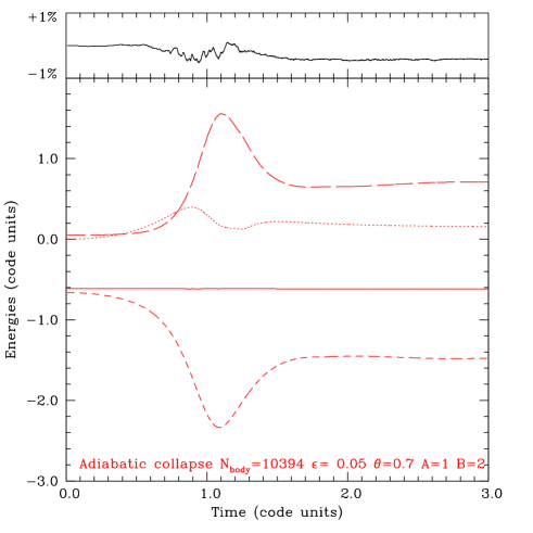
Figure 3: Energy trend in the adiabatic collapse. The dashed-dotted line indicates potential energy, the dotted line kinetic, the dashed line thermal, and the solid line total energy. The top panel is a zoom on the trend of total energy, showing the deviation from perfect conservation.

Table 1: The Adiabatic Collapse test. Benchmarks for a run with $2\times 10^{4}$ particles. Time refers to 50 time-stpes.

$N_{cpu}$	Total	Data Up-date	Parallel Over-head	Neighbors	SPH	Gravity	Miscellaneous
	secs	secs	secs	secs	secs	secs	secs
1	120	0.47	0.00	40	36	40	3.53
2	69	0.22	0.60	23	19	25	1.18
4	42	0.27	1.70	14	9.5	15	1.53
8	23	0.13	3.20	5.5	5.4	5.3	3.47
16	17.3	0.13	3.40	3.4	3.0	3.8	3.60
32	11.5	0.09	3.00	2.6	1.3	3.2	1.31
64	7.5	0.05	2.90	0.33	1.1	1.9	1.23

5.2 Description of the tests

The state of the system at the time of the maximum compression is shown in the various panels of Fig. 1, which displays the density, radial velocity, pressure and specific internal energy profiles. Each panel shows the variation of the physical quantity under consideration (in suitable units) as a function of the normalized radial coordinate at time equal to 0.88 .

The initial low internal energy is not sufficient to support the gas cloud which starts to collapse. Approximately after one dynamical time scale a bounce occurs. The system afterwards can be described as an isothermal core plus an adiabatically expanding envelope pushed by the shock wave generated at the stage of maximum compression. After about three dynamical times the system reaches virial equilibrium with total energy equal to a half of the gravitational potential energy (Hernquist & Katz 1989). The temporal evolution of the kinetic, thermal and potential energies, is shown in Fig. 2. The trends are quite similar to Steinmetz & Ml̈ler (1993) and Hernquist & Katz (1989). Total energy conservation, measured as the maximum deviation from the perfect conservation, is ensured below $1\%$.

The present results agree fairly well with the mean values of the Hernquist & Katz (1989) simulations, which in turns agree with the 1D finite difference results (Evrard 1988). As an example, the shock is located at the radial distance $0.18\leq r/R\leq 0.25$ in the models at $t\approx 0.88$ (cf. the velocity panels of Fig.1) . The good agreement between the results of the parallel and scalar tests guarantees that the processors exchange data correctly. The level of precision can be gauged by estimating the effect of the interpolation stage (which we use to avoid an additional communication flow) on the evaluation of the thermal energy. To this aim we run the adiabatic collapse test with the scalar and parallel (8 cpus) code, by imposing that all the particles are active. This indeed represents the most non uniform situation. It turns out that the deviation due to the interpolation amounts at maximun to $0.8\%$. The maximum deviation is located at the time of the maximum compression (t  $\approx$  0.88).

Figure 4: Scalability of different code sections (solid lines), as reported in each panel, averaged on 50 time-steps. Dashed lines indicate the ideal scalability.

6 Benchmark

To evaluate the code performances, we use the adiabatic collapse just described, and perform simulations at increasing number of processors. We believe that this test is very stringent, and can give a lower limit of the code performances due to the high density contrast that is present at the time of maximum compression, when the particles are highly clustered. We are going to check the code timing, overall load-balance and scalability. Moreover we shall analyze in details particular sections of the code, like the gravity computations,the SPH and the neighbor searching. An estimate of the parallel over-head will be given as well.

6.1 Timing analysis

We run the adiabatic collapse test up to the time of the maximum compression (t $\simeq 1.1$) using $2\times 10^{4}$ particles on 1, 2, 4, 8, 16, 32 and 64 processors, and looked at the performances in the following code sections (see also Table 1):

$\bullet$

total wall-clock time;

$\bullet$

data up-dating;

$\bullet$

parallel computation, which consists of barriers, the construction of the ghost-tree and the distribution of data between processors;

$\bullet$

search for neighbor particles;

$\bullet$

evaluation of the hydro-dynamical quantities;

$\bullet$

evaluation of the gravitational forces;

$\bullet$

miscellaneous, which encompasses I/O and statistics.

The results summarized in Table 1 present the total wall-clock time per processor over the last 50 time-steps, together with the time spent in each of the 5 subroutines (data updating, neighbor searching, SPH computation, gravitational interaction and parallel computation). The gravitation interaction takes about one-third of the total time, while the search for neighbors takes roughly comparable time. The evaluation of hydrodynamical quantities (see Section 3.5) takes about one-fourth of the time, the remaining time being divided between I/O and data up-dating. The parallel over-head does not appear to be a serious problem, being at maximum about $1\%$ of the total time. This timing refers, as indicated above, to simulations stopped at roughly the time of maximum compression. A run with 8 processors up to $t\simeq 2.5$, the time at which the system is almost completely virialized, took 3800 secs. Global code performances are analyzed in the next sections.

Figure 5: Overall code load-balance, averaged on 50 time-steps (solid line). Dashed line indicates ideal load-balance.

Figure 6: Overall code scalability, averaged on 50 time-steps (solid line). Dashed line indicates ideal scalability.

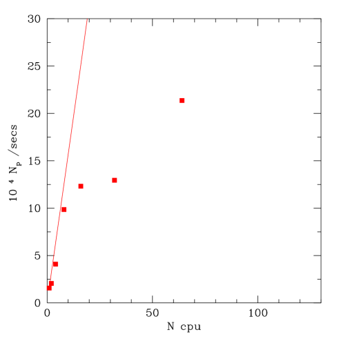
Figure 7: Code scalability in a pure collisionless simulation. See text for more details.

6.2 Load-balance

One of the most stringent requirements for a parallel code is the capability to distribute the computational work equally between all processors. This can be done defining a suitable work-load criterion, as discussed in Section 3.2. This is far from being an easy task (Davè et al 1997), and in practice some processors stand idly for some time waiting that the processors with the heaviest computational load accomplish their work. This is true also when an asynchronous communication scheme is adopted, as in our TreeSPH code. As outlined in Section 3.2, we are using individual work-loads, based on the time spent to evaluate the gravitational interaction on one particle with all the other ones. A better choice would be to define the work-load only for active particles, which are the particles evolving fatly. This possibility is currently under investigation, due to the memory problems that can arise, as discussed in Section 3.5. To evaluate the code load-balance we adopted the same strategy of Davè et al (1997), measuring the fractional amount of time spent idle in a time-step while another processor performs computation:

$$L=\frac{1}{N_{procs}}\sum_{j=1}^{N_{procs}}1-\frac{(t_{max-t_{i}})}{t_{max}}.$$ (21)

Here $t_{max}$ is the time spent by the slowest processor, while $t_{i}$ is the time taken by the $i-th$ processors to perform computation. The results are shown in Fig 5, where we plot the load-balance for simulations at increasing number of processors, from 1 to 64. The load balance maintains always above $80\%$, being close to 1 up to 8 processors. For the kind of simulations we are performing, the use of 8 processors is particularly advantageous for symmetry reasons.

6.3 Scalability

At increasing number of processors, a parallel code should ideally speed up linearly In practice the increase of the processors number causes an increase of the communications between processors, and a degradation of the code performances. To test this, we used the same simulations discussed above, running the adiabatic collapse test with $2\times 10^{4}$ particles at increasing processors number. We estimated how the code speed scales computing the wall-clock time per processor spent to execute a single time-step, averaged over 50 time-steps. In Fig. 6 we plot the speed (in $sec^{-1}$) against the number of processors.
The code scalability keeps very close to the ideal scalability up to 8 processors, where it shows a minimum. This case in fact is the most symmetric one Then the scalability deviates significantly only when using more that 16 processors. Looking also at Fig. 4, it is easy to recognize that mainly the gravitational interaction is responsible for this deviation.

To better judge the code performances, we run a simulation of the collapse of a pure DM system, aiming at showing the scalability of the gravity section of the code. The results are shown in Fig.  7. They are good up to 16 processors, afterwards they suddenly get worse. This trend does not change by introducing all the other code parts, as it will be shown in the next sections. This is clearly imputable to the dominant role of the gravity, which represents not only the most time consuming section of any TreeSPH code (this holds also for the serial code), but also by definition the less parallel part of the code.

In the next Sections we are going to investigate whether the code overall performances might improve adding new physics (like cooling and star formation) which is necessary to describe the evolution of real systems, like galaxies.

6.4 Memory considerations

Together with the efficiency, considerations on the memory use of a parallel code are crucial (Davè et al 1998). A good use of the memory can significantly reduce the communication overhead. In fact, by increasing the number of particles per processor, the local computation increases with respect to the remote one, decreasing the amount of time spent commnicating. In our case, any T3E processor possesses 16 Megawords (128 Mbyte) of memory. Our parallel code can manage roughly 100 K particles per processor, roughly 1.8 times less than the serial code. Therefore our code is not perfectly optimized as far as memory is concerned. This is due partly to the fact that with respect to Davè et al (1997) we use twice the number of neighbours, and by the fact that we did not pose much restrictions on th extension of the ghost-tree aiming at limiting the number of communications.

7 Adding new physics

In this section we are going to present the collapse of a mix of DM and baryons, with and without cooling. Firstly we show how cooling is implemented in our Tree-SPH code, and how the integration of the energy equation is performed. Then we show a simple model for the formation of a spiral galaxy, and then we discuss the code performances when cooling is included.

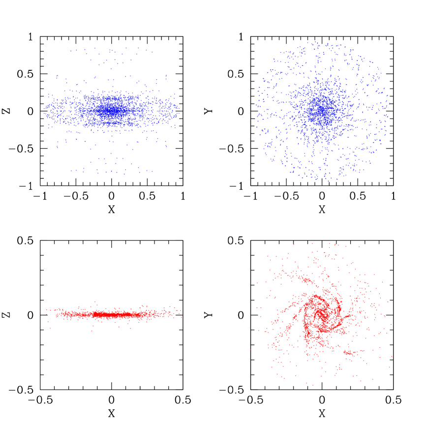
Figure 8: The collapse of a spherical mix of DM and gas with cooling. Upper panels show the final DM distribution, whereas lower panels show the gas distribution. The $X-Z$ projection is on the right, while the $X-Y$ one on the left.

7.1 On the integration of the energy equation

The usual form of the energy equation in SPH formalism is

$$\frac{du_{i}}{dt}=\sum_{j=1}^{N}m_{j}\left(\frac{\sqrt{P_{i}P_{j}}}{\rho_{i}\rho_{j}}+\frac{1}{2}\Pi_{ij}\right){\bf v}_{ij}\cdot$$

$$\frac{1}{2}\left({\vec{\nabla}}_{i}W(r_{ij},h_{i})+\vec{\nabla}_{i}W(r_{ij},h_{j})\right)+\frac{\Gamma-\Lambda_{C}}{\rho},$$ (22)

(Benz 1990; Hernquist & Katz 1989). The first term represents the heating or cooling rate of mechanical nature, whereas the second term $\Gamma$ is the total heating rate from all sources apart from the mechanical ones, and the third term $\Lambda_{C}/\rho$ is the total cooling rate by many physical agents (see Carraro et al. 1998a for details).

In absence of explicit sources or sinks of energy the energy equation is adequately integrated using an explicit scheme and the Courant condition for time-stepping (Hernquist & Katz 1989).

The situation is much more complicated when considering cooling. In fact, in real situations the cooling time-scale becomes much shorter than any other relevant time-scale (Katz & Gunn 1991), and the time-step becomes considerably shorter than the Courant time-step. even using the fastest computers at disposal. This fact makes it impossible to integrate the complete system of equations (cf. Carraro et al. 1998a) adopting as time-step the cooling time-scale.

To cope with this difficulty, Katz & Gunn (1991) damp the cooling rate to avoid too short timesteps allowing gas particles to loose only half of their thermal energy per timestep.

Hernquist & Katz (1989) and Davé et al. 1997 solve semi-implicitly eq. (22) using the trapezoidal rule,

$$u_{i}^{n+1}=u_{i}^{n}+\frac{1}{2}(dt_{i}^{n}\times e_{i}^{n}+dt_{i}^{n+1}\times e_{i}^{n+1}).$$ (23)

The leap-frog scheme is used to update thermal energy, and the energy equation, which is nonlinear for $u_{j}$, is solved iteratively both at the predictor and at the corrector phase. The technique adopted is a hybrid scheme which is a combination of the bi-section and Newton-Raphson methods (Press et al 1989). The only assumption is that at the predictor stage, when the predicted $\tilde{u}_{i}^{n+1}$ is searched for, the terms $u_{i}^{n+1}$ are equal to $u_{i}^{n-1}$.

Our scheme to update energy is conceptually the same, but differs in the predictor stage and in the iteration scheme adopted to solve equation 23.

In brief, at the first time-step the quantity $u^{n-1/2}$ is calculated and for all subsequent time steps, the leap-frog technique, as in Steinmetz & Müller (1993), is used:

(i) We start with $u^{n}$ at $t^{n}$;

(ii) compute $\tilde{u}^{n}$ as

$$~{}~{}~{}~{}~{}~{}~{}~{}~{}~{}\tilde{u}^{n}=u^{n-1/2}+\frac{1}{2}t^{n}\times e^{n}$$

where $e_{i}=du_{i}/dt$. This predicted energy, together with the predicted velocity is used to evaluate the viscous and adiabatic contribution on $e_{i}^{n+1}$. In other words the predictor phase is calculated explicitly because all the necessary quantities are available from the previous time step $t^{n}$.

(iii) finally, derive $u^{n+1}$ solving the equation 23 iteratively (corrector phase) for both the predicted and old adiabatic and viscous terms;

Figure 9: The collapse of a spherical mix of DM and gas without cooling. Upper panels show the final DM distribution, whereas lower panels show the gas distribution. The $X-Z$ projection is on the left, while the $X-Y$ one on the right.

In the corrector stage the integration of the equation 23 is performed using the Brent method (Press et al 1989) instead of the Newton-Raphson, the accuracy being fixed to a part in $10^{-5}$. The Brent method has been adopted because it is better suited as root–finder for functions in tabular form (Press et al. 1989).
Radiative cooling is implemented as in Carraro et al 1998a. We adopt cooling functions from Sutherland and Dopita (1993), which are tabulated as a function of metallicity. Tables are available for metallicity from $Z=10^{-5}$ to $Z=0.5$.

The parallel implementation of the radiative cooling does not present any special difficulties. For each particle in fact there are already at disposal all the necessary quantities (temperature and density, basically) to evaluate the amount of energy loss by cooling processes. Only that in our code the overall efficiency is improved on making the faster processors to compute the amount of radiated energy not only for their own particles, but also for the particles residing inside the slower processors. This allows us to achieve a much better global load-balance (sse below).

Figure 10: Scalability of different code sections (solid lines), as reported in each panel, averaged on 50 time-steps. Dashed lines indicate the ideal scalability.

Figure 11: Overall code load-balance, averaged on 50 time-steps (solid line) for the simulations described in Section 7.2 . Open squares refer to a simulation in which cooling is turned off, whereas filled squares refer to a simulation in which cooling is switched on. The dashed line indicates ideal scalability.

Figure 12: Overall code scalability, averaged on 50 time-steps (solid line) for the simulations described in Section 7.2. Open squares refer to a simulation in which cooling is turned off, whereas filled squares refer to a simulation in which cooling is switched on. The dashed line indicates ideal load-balance.

7.2 The Formation of a disk-like galaxy

We consider a spherical DM halo whose density profile is

$$\rho(r)\propto\frac{1}{r}.$$ (24)

Although rather arbitrary, this choice seems to be quite reasonable. Indeed DM halos emerging from cosmological N–body simulations are not King or isothermal spheres, but show, independently from cosmological models, initial fluctuations spectra and total mass, a universal profile (Huss et al 1998). This profile is not a power law, but has a slope $\alpha=dln\rho/dlnr$ with $\alpha=-1$ close to the halo center, and $\alpha=-3$ at larger radii. Thus in the inner part the adopted profile matches the universal one. Moreover this profile describes a situation which is reminiscent of a collapse within an expanding universe, being the local free fall time a function of the radius (see for instance the discussion in Curir et al 1993).

DM particles are distributed in a regular cubic grid inside a sphere of unitary radius (Carraro et al 1998a). The radial density profile in eq. (5) is realized stretching the initial grid (see eq. 20).
To mimic the cosmological angular momentum acquisition by tidal torque with the surrounding medium we put the halo in solid body rotation around the z-axis with an angular rotation velocity $\omega~{}=~{}0.5~{}sec^{-1}$, which corresponds to $\lambda$  =  $0.09$, where

$$\lambda=\frac{J|E|^{1/2}}{GM^{5/2}}$$

is the dimensionless spin parameter used to characterize the amount of angular momentum in bound systems. $J$ is the total angular momentum of the system, $E$ is the binding energy, $M$ is the total mass, and $G$ is the gravitational constant, kept equal to $1$ in our simulations. $\lambda$ equal to $0.05$ is quite typical for halos emerging from cosmological N–body simulations (Katz 1992, Steinmetz & Bartelmann 1996).

For the simulations here described we used $10^{4}$ dark particles and $10^{4}$ gas particles. The softening parameter $\epsilon$ is computed as follows. After plotting the inter-particles separation as a function of the distance to the model center, we compute $\epsilon$ as the mean inter-particles separation at the center of the sphere, taking care to have at least one hundred particles inside the softening radius (Romeo A. G. 1997). We consider a Plummer softening parameter and keep it constant along the simulation. It turns out ot be $5\times 10^{-3}$ .
To mimic the infall of gas inside the potential well of the halo, we distribute gas particles on the top of DM particles. The baryonic fraction adopted is $f_{b}~{}=0.1~{}$, and gas particles are Plummer–softened in the same way as the DM particles.
Under cooling and because of the velocity field of the halo, the gas is expected to settle down in a rotating thin structure.
The results are shown in Fig. 8, where upper panels refer to the evolution of the dark component, whereas lower panels refer to the gas. Left panels show the evolution in the $X-Z$ plane, while right panels show the evolution in the $X-Y$ plane. Due to the spin the dark halo flattens (upper-left panel), whereas the gas settles in a thin disk (bottom-left panel) which exhibits some spiral arms (lower-right panel).
These results are similar to those we have obtained with our scalar Tree-SPH code (Lia et al 1999).
This simulation is by no means aimed at producing a real disk, but only to show that cooling is properly implemented.

A similar series of simulations, but without cooling, have been run, aiming at checking how the code performances change including new physics. In brief, we run the same simulation switching cooling off. The result is shown in Fig 9. As expected without cooling, the gas component keeps round-shaped, whereas DM gets flatter in the $X-Z$ plane (Carraro et al 1998a, Navarro & White 1993).

7.3 Benchmark

As for the adiabatic collapse we run a series of simulations of the formation of a disk galaxy at increasing number of processors.
We show the results in term of scalability and load balance in Figs 10, 11 and 12. In Fig. 11 we present the scalability of 3 different code sections, namely the gravity computation, the neighbors searching and the SPH, measured as the wall-clock time spent in a certain subroutine normalized to the global time-step, at increasing number of processors. Looking at this figure, we conclude that the inclusion of the cooling processes does not affect the scalability. The most significant deviation is visible in the gravity part of the code, like in the case of the adiabatic collapse (see Section 6), where the scaling starts deviating significantly from the ideal one when using more than 32 processors.

On the other hand, the SPH and neighbors searching parts of the code scale very well up to 64 processors. The parallel over-head, which measures the time spent to synchronize the processors, increases with the number of cpus, but always keeps below $10\%$.
In Figs 11 and 12 we compare the overall scalability and load-balance comparing a simulation of a galaxy collapse with (see Fig. 8) and without cooling (see Fig. 9). Filled squares represent the load-balance trend for the case of a collapse with cooling turned on, whilst open squares refer to simulations in which cooling is turned off.

From Fig. 11, it turns out that the inclusion of the cooling processes sensibly improves on the global load-balance. This means that our parallel scheme to calculate cooling partially alleviates computing time differences between fast and slow processors. This improvement is clearly due to the fact that the fastest processors compute the amount of energy radiated away by cooling also for the particles residing in the slowest processors. Going into some details, when a fast processor has completed all the computation for its own particles, by using a SHMEM directive shmem-int4-finc it computes cooling for slower processors, which are still working.
The two curves keep close up to 16 processors, afterwards they start to deviate.
Fig. 12 presents the global code scalability for the two cases. No difference can be outlined in the two series of simulations, showing that the inclusion of cooling does not slow down the code, at odd with what occurs in the serial code. A clear departure from the ideal scalability starts when using more than 16 processors.

We consider these results quite encouraging, also comparing our findings with Davé et al (1997, see their Fig. 6) ones as far as scalability is concerned.

8 A spherically symmetric proto-cluster collapse

Following Evrard (1988) step by step we simulate the turn-around and collapse of a spherical perturbation in a flat cosmology ($\Omega=1.0$) where the mass fraction of baryons over Dark Matter is $f_{b}=0.1$.

8.1 Initial conditions

We generate an initial perturbation consisting of a single radial cosine wave (Peebles 1982).
Given a uniform sphere of radius $x_{t}$, one perturbs comoving radii by

$$\vec{x}_{0}\rightarrow\vec{x}_{1}=x_{0}\times(1-\delta(x_{0})/3)$$ (25)

and sets peculiar velocities according to growing linear theory

$$\vec{v}=-\frac{2}{3}H\vec{x}_{0}\delta(x_{0})$$ (26)

where

$$\delta(x)=0.5\delta_{0}\times[1+cos(\pi x/x_{t})].$$ (27)

Figure 13: Evolution of the gas in the X-ray cluster collapse. Upper panels show the evolution of temperature, middle panels pressure and radial velocity, lower panels density. The results are shown for z = 4.00, 1.39, 0.97, 0.50, 0.24 and 0.00.

Figure 14: Redshift evolution of the core properties of the simulated cluster. The core radius $r$, enclosed gas mass $M$, mean gas temperature $T$ and total X-ray luminosity ( in $10^{43}~{}erg~{}sec^{-1}$ ) are shown.

The initial perturbation has $\delta_{0}=1$ and it is scaled to a size appropriate to rich cluster of galaxies. The cosmological parameter of the simulation are:

$\bullet$

mean density $\Omega$ = 1.0 ;

$\bullet$

Hubble constant $H_{0}$ = 50$Km~{}sec^{-1}~{}Mpc^{-1}$ ;

$\bullet$

baryon density (in units of the critical density) $\Omega_{b}$ = 0.1.

We used 100,000 gas particles and an equal number of collisionless DM particles within $x_{t}$. The model is evolved starting from $z=4.0$, the total mass being $M_{t}=3\times 10^{15}M_{\odot}$. The corresponding comoving radius is $x_{t}\approx 22~{}Mpc$ assuming $H_{0}=50~{}Km~{}sec^{-1}~{}Mpc^{-1}$. The gas has an initial temperature of $10^{5}~{}^{o}K$. Since the density perturbation is zero at $x=x_{t}$, the outer edges expand freely. We adopt a gravitational softening parameter $\epsilon\approx 5~{}kpc$.

8.2 Results

The simulation here presented was run using 32 processors and the full evolution required about 11 node-hours.
The detailed evolution of the baryonic component is shown in Fig 13, where we plot in natural units (c.g.s.) the system number density, radial velocity, pressure and temperature at the same redshifts of Evrard (1988), namely $z$ = 4.00, 1.39, 0.97, 0.50, 0.24 and 0.00 .

The results agree well with Evrard (1988), who used about 3500 particles in total, but are much closer to the 1D lagrangian finite difference results reported by Evrard (1988) due to the much higher resolution of our simulation. In particular the shock front is always very well defined, and at $z=0$ our profiles match fairly well the 1D ones (see Evrard, 1988 Fig 8), especially at the center, which we succeed to resolve much better.

We finally compare the redshift evolution of the cluster core properties to obtain a further check of the reliability of our results. First of all we define the cluster core radius as the radius at which the mean interior density equals a constant value times the background density at that redshift. The constant value has been chosen to be 170 to be consistent with Evrard (1988).

For the output redshifts Fig. 14 shows the results for the redshift evolution of the core radius (in $Mpc$), the enclosed baryonic mass (in $M_{\odot}$), the mean gas temperature (in ${}^{o}K$) and the total X-ray luminosity, in units of $10^{43}erg~{}sec^{-1}$. We find a nice agreement with the 1D calculation presented by Evrard (see his Fig. 10). In particular thanks to our higher resolution, we find good agreement also for the total X-ray luminosity.

9 Summary and future perspectives

In this paper we have presented a new parallel implementation of a Tree-SPH code, realized by means of the SHMEM communications libraries for a 256 processors T3E massively parallel computer.

We have shown that the code performs quite well against several well known tests, like the adiabatic collapse of an initially isothermal gas sphere and the spherical symmetric proto-cluster of galaxies collapse.

The qualitative results achieved and the global code load-balance and scalability are particularly encouraging.
The code is not portable at present, but it will be in the near future when MPI 2 will be released. This way the code can be run also on different machines, like for instance the IBM SP3, the new IBM parallel machine based on Power 3 cpus. We believe that simulations of galaxy clusters formation which include cooling and star formation are feasible using up to half a million particles of gas and an equivalent number of collisionless particles.

We plan to use our code to address many different issues related to Galaxy Formation, like for instance the formation of elliptical galaxies, the interaction between Dark Matter and baryons at galactic scale, and the structure and evolution of Damped Lyman $\alpha$ clouds.

References

- [1] Aarseth S.J., 1985, in ‘Multiple Time Scales’, ed J. Brackill and B.I. Cohen (New York:Academic), p. 377
- [2] Aarseth S.J., 1998, IAU Colloquium 172
- [3] Appel A.W., 1985, SIAM J. Sci. Stat. Comp. Phys. 12, 389
- [4] Balsara D.S., 1995, J. Chem. Phys. 121, 357
- [5] Barnes J.E., Hut P., 1986, Nature 324, 446
- [6] Barnes J.E., 1994, in ’Computational Astrophysics’, eds. J. Barnes et al, Berlin, Springer-Verlag
- [7] Benz W., 1990, in Numerical Modelling of Nonlinear Stellar Pulsation, ed. J. R. Buchler, p. 269, Dordrecht: Kluwer
- [8] Baugh C.M., Cole S., Frenk C.S., Lacey C.G., 1998, ApJ 498, 504
- [9] Bravo E., Garcia-Senz D., 1995, ApJ 450, L17
- [10] Bryan G.L., Norman M.L., 1995, AAS Bull. 187, 9504
- [11] Buonomo F., Carraro G., Chiosi C., Lia C., 1999, MNRAS in press (astro-ph/9909199)
- [12] Carraro G., Lia C., Chiosi C., 1998a, MNRAS 297, 1029
- [13] Carraro G., Lia C., Buonomo F., 1998b, in ”DM-Italia 1997”, ed. P. Salucci, Studio Editoriale Fiorentino, p. 169
- [14] Curir A., Diaferio A., De Felice F., 1993, ApJ 413, 70
- [15] Davé R., Dubinski J., Hernquist L., 1997, New Astronomy 2(3), 277
- [16] Davis M., Efstathiou G., Frenk C.S., White S.D.M., 1985, ApJ 292, 371
- [17] Dubinski J., 1996, New Astronomy 1, 133
- [18] Evrard A.E., 1988, MNRAS 235, 911
- [19] Evrard A.E., 1990, ApJ 363, 349
- [20] Gheller C., Pantano O., Moscardini L., 1998a, MNRAS 285, 519
- [21] Gheller C., Pantano O., Moscardini L., 1998b, in ‘Science and Super Computing at CINECA - Report 1997’, p. 37
- [22] Gingold R.A., Monaghan J.J., 1977, MNRAS 181, 375
- [23] Glanz J., 1998, Science 280, 1522
- [24] Hernquist L., 1987, ApJS 64, 715
- [25] Hernquist L., Katz N., 1989, ApJS 70, 419
- [26] Hernquist L., Katz N., Weinberg D.H., Miralda-Escudé J., 1996, ApJ 457, L51
- [27] Hockney R.W., Eastwood J.W., 1981, Computer Simulation using Particles, McGraw Hill, New York
- [28] Huss A., Jain B., Steinmetz M., 1998, ApJ 517, 64
- [29] Hut P., Makino J., 1999, Science, Vol. 283, 501
- [30] Kang H., Ostriker J. P., Cen R., Ryu D., Hernquist L., Evrard A. E., Bryan G. L., Norman M. L., 1994, ApJ 430, 83
- [31] Katz N., Gunn J. E., 1991, ApJ 377, 365
- [32] Katz N., 1992, ApJ 391, 502
- [33] Katz N., White S.D.M., 1993, ApJ 412, 455
- [34] Katz N., Weinberg D.H., Hernquist L., 1996, ApJS 105, 19
- [35] Kauffmann G., White S.D.M., Guiderdoni B., 1993, MNRAS 264, 201
- [36] Landau L., Lifchitz E., 1971, Fluid Mechanics, Mir Edition, Moscow
- [37] Lia C., Carraro G., 1999, Proceedings of the Euroconference ”The Evolution of Galaxies on Cosmological Timescales”, Puerto de la Cruz, Tenerife, Spain, Nov 30 - Dec 5 1998
- [38] Lucy, L., 1977, AJ 82, 1013
- [39] Mihos J. C., Hernquist L., 1994, ApJ 437, L47
- [40] Monaghan J.J., 1992, ARA&A 30, 543
- [41] Monaghan J.J., Lattanzio J.C., 1985, A&A 149, 135
- [42] Monaghan J.J., Lattanzio J.C., 1991, ApJ 375, 177
- [43] Moore B., Governato F., Quinn T., Stadel J., Lake G. 1998, ApJ 499, L5
- [44] Navarro J.F., White S.D.M., 1993, MNRAS 265, 271
- [45] Navarro J.F., Frenk C.S., White S.D.M., 1996, ApJ 462, 563
- [46] Navarro J.F., Steinmetz M., 1997, ApJ 478, 13
- [47] Pearce F.R., Couchman H.M.P., 1997, New Astronomy 2, 411
- [48] Peebles P.J.E., 1982, ApJ 257, 438
- [49] Peebles P.J.E., 1993, Principles of Physical Cosmology, Princeton Series in Physics
- [50] Press W.H., Flannery B.P., Teukolsky, S.A., Vetterling, W.T., Numerical Recipes, 1989, Cambridge: Cambridge University Press
- [51] Romeo A.B., 1997, A&A 324, 523
- [52] Salmon J., 1991, PhD Thesis, Caltech
- [53] Shapiro P.R., Martel H., Villumsen J.V., Owen J.M., 1996, ApJS 103, 269
- [54] Sigurdsson S., He B., Melhem R., Hernquist L., 1997, Computers in Physics 11, 4
- [55] Steinmetz M., Müller E., 1993, A&A 268, 391
- [56] Steinmetz M., 1996, in ”New light on Galaxy Evolution”, eds. R. Bender & R. L. Davies, p. 259, Dordrecht: Kluwer Academic Press
- [57] Sutherland R.S., Dopita M.A., 1993, ApJS 88, 253
- [58] Thornton K., Gaudlitz M , Janka H-T, Steinmetz M., 1998, ApJ, 500, 95
- [59] White S.D.M., Rees M.J., 1978, MNRAS 183, 341
- [60] Woodward P., Colella P., 1984, J. Comput. Phys. 54, 115