The Globular Cluster Systems in the Coma Ellipticals. II: Metallicity Distribution and Radial Structure in NGC 4874, and Implications for Galaxy Formation

Abstract

Deep HST/WFPC2 images in $V$ and $I$ are used to investigate the globular cluster system (GCS) in NGC 4874, the central cD galaxy of the Coma cluster. Although the luminosity function of the clusters displays its normal Gaussian-like shape and turnover level, other features of the system are surprising. We find the GCS to be (a) spatially extended, with core radius $r_{c}\sim 22$ kpc, (b) entirely metal-poor (a narrow, unimodal metallicity distribution with $\langle$[Fe/H]$\rangle\sim-1.5$), and (c) modestly populated for a cD-type galaxy, with specific frequency $S_{N}=3.7\pm 0.5$. Model interpretations suggest to us that as much as half of this galaxy might have accreted from low-mass satellites, but no single one of the three classic modes of galaxy formation (accretion, disk mergers, in situ formation) can supply a fully satisfactory model for the formation of NGC 4874. Even when they are used in combination, strong challenges to these models remain. We suggest that the principal anomaly in this GCS is essentially the complete lack of metal-rich clusters. If these were present in normal (M87-like) numbers in addition to the metal-poor ones that are already there, then the GCS in total would more closely resemble what we see in many other giant E galaxies. This supergiant galaxy appears to have avoided forming globular clusters during the main metal-rich stage of star formation which built the bulk of the galaxy.

1 Introduction

NGC 4874 is the central cD-type galaxy in the rich Coma cluster. As such, it presents a rare opportunity for us to study the characteristics of a globular cluster system (GCS) in an extreme environment: a host galaxy which is near the very top end of the luminosity scale and is within an extremely rich environment of other galaxies. The characteristics of the GCS including the metallicity distribution (MDF) of the clusters, the specific frequency of the cluster system, its spatial structure, and the luminosity distribution of the clusters, all provide distinctive clues to the evolutionary history of the galaxy (see, e.g., Harris (1991), 1999 and Ashman & Zepf (1998) for extensive reviews).

In Paper I (Kavelaars et al.  (1999)), we described new imaging observations of NGC 4874 taken with the WFPC2 cameras on board HST, and discussed the luminosity distribution function (GCLF) of the globular clusters. Here, we discuss the spatial distribution of the clusters, the MDF, and the specific frequency, and we describe how they may constrain competing scenarios for the formation history of this unusual system.

The raw WFPC2 data for this program (GO-5905) consisted of $V$ (F606W) exposures totalling 20940 sec, and $I$ (F814W) exposures totalling 8720 sec. NGC 4874 was approximately centered in the PC1 chip to maximize the total globular cluster population falling within our field of view. A complete description of the data reduction procedures, including DAOPHOT and ALLFRAME measurement, photometric transformations, and artificial-star tests of the photometric error and completeness functions, is given in Paper I.

In Figure 1 we show the WFPC2 field with the locations of the brightest detected objects. The $y-$axis of the array is directed $59\fdg 0$ east of north. In total, 4313 objects classified as “starlike” in structure (consisting of globular clusters around NGC 4874, some faint very compact background galaxies, and a very few foreground field stars) were measured in $V$. Of these, 3344 were also measured in $I$ and thus $(V-I)$. The concentration of objects around NGC 4874 is evident, but the distribution is much less centrally concentrated than (for example) around another large Coma elliptical, IC 4051 (Woodworth & Harris (1999)).

In Paper I, the distribution in $V$ magnitude (the GCLF) was employed to determine the distance modulus to the Coma cluster and an estimate of the Hubble constant. We found the GCLF “turnover” point to lie at $V=27.88\pm 0.12$, leading to $\mu_{0}$(Coma) $=35.05\pm 0.12$ and $H_{0}=69\pm 9$ km s^-1 Mpc^-1. In the discussion of this paper, we will simply assume a Coma distance $d=100$ Mpc to convert any angular measurements into linear ones.

The color-magnitude diagram for all objects with measured $(V-I)$ color indices is shown in Figure 2. Since the $I$ frames had relatively short total exposure time, this color distribution does not quite reach the turnover point, and fainter than $V\sim 26$ the appearance of the diagram is dominated by the random measurement uncertainty of the photometry. We will discuss the color (metallicity) distribution in more detail in section 4 below.

2 The Radial Distribution: A Galactic or Intergalactic GCS?

Pioneering attempts to measure the NGC 4874 GCS from ground-based CFHT imaging (Harris (1987); Thompson & Valdes (1987)) succeeded in resolving the brightest clusters and hinted that their radial distribution was surprisingly flat, with the surface density of clusters $\sigma_{cl}$ falling off with radius as $\sim r^{-1}$ for $r\,{}^{>}_{\sim}\,20^{\prime\prime}$. Our new HST data cover a similar radial range but of course penetrate considerably deeper. To obtain the radial profile of the GCS, we subdivided the WFPC2 field into several annuli and calculated the number density of starlike objects down to an adopted cutoff magnitude $V=27$, above which the detection incompleteness was small. The results are summarized in Table 1 and shown in Figure 3. In the Table, successive columns give (1) the mean radius of each annulus, (2) the number of starlike objects within the annulus, after (small) completeness corrections, (3) the area $A$ of the annulus that falls within the WFPC2 boundaries, and (4) the projected number density of starlike objects, $\sigma=n/A$. Column (5) gives the deduced mass density after deprojection into three dimensions, as described below.

The projected density $\sigma$ declines smoothly and slowly outward from the galaxy center and is still declining at the edges of our WFPC2 field ($r\sim 120^{\prime\prime}$ corresponds to almost 60 kpc linear radius). Plainly, the GCS of this giant galaxy spills past the borders of our field, making it difficult to estimate the surrounding background level $\sigma_{b}$ from our data alone. However, without knowing $\sigma_{b}$ we cannot obtain the true profile of the GCS. Lacking any true “control” field adjacent to NGC 4874, we have instead used data from another Coma field, the elliptical galaxy IC 4051 (Woodworth & Harris (1999)), in which the magnitude limits, data reduction procedures, etc., are all closely comparable to ours. Fortunately, the IC 4051 GCS is much more centrally concentrated, so that the starcounts in the outer regions of its WFPC2 field are very close to the true surrounding background. We adopt $\sigma_{b}=(0.02\pm 0.005)$ arcsec^-2 – about one-third the projected density of the outermost parts of our NGC 4874 field – and subtract this from the entries in Table 1 to obtain the profile plotted in Fig. 3.

Notably, the slope of the $\sigma_{cl}(r)$ curve steepens outward, continuously from $r\sim 10^{\prime\prime}$ (or $\simeq 5$ kpc) all the way out to $r\sim 120^{\prime\prime}$ (60 kpc). The flat inner-halo core is remarkably extended, and the outer halo does not follow a single power-law exponent as well as in several other giant ellipticals at the centers of rich clusters (e.g., Harris 1986, 1991; Blakeslee (1999)). The steepening of the profile past $r\sim 120^{\prime\prime}$ hints that the outer halo there may become truncated (because of tidal interactions with the other large Coma ellipticals?). This dropoff in $\sigma_{cl}$ is not just an artifact of our adopted background level: it would still be present even if we had arbitrarily adopted $\sigma_{b}=0$, as shown by the open circles in Fig. 3.

The profile of the halo light of NGC 4874 has been measured via CCD photometry to comparable radii by Peletier et al.  (1990) and Jorgensen et al.  (1992). In Fig. 3 we compare their data with the GCS profile. The halo surface intensity is well described by a simple power law $\mu$(halo) $\sim r^{-1.1}$ over the range $5^{\prime\prime}\,{}^{<}_{\sim}\,r\,{}^{<}_{\sim}\,90^{\prime\prime}$ (see particularly the Peletier et al. $R-$band data, which cover the largest radial range. NGC 4874 is well known to be a difficult target for wide-field surface photometry, since at radii beyond $100^{\prime\prime}$ or so, its halo light becomes confused with the light from several neighboring large ellipticals in the Coma core region.). However, the GCS profile does not fit such a simple description: its slope steepens continuously outward, and it can be claimed to match the halo light profile only for $r\,{}^{>}_{\sim}\,40^{\prime\prime}$.

Very few other giant ellipticals, even cD types, have GCS profiles this extended. Other roughly comparable cases may include NGC 3311, the very diffuse central cD in Hydra I (Harris (1986); McLaughlin et al.  (1995)), perhaps NGC 6166, the cD in Abell 2199 (Pritchet & Harris (1990)), and some of the Abell-cluster central giants studied by Blakeslee (1999) , particularly A754. We have used standard King (1966) model fits to the GCS radial distribution in order to obtain formal estimates of the core radius of the projected profile. Over a wide range of assumed central concentration parameters, we find $r_{c}\simeq 45^{\prime\prime}$ (corresponding to 22 kpc). By contrast, the core radius of the halo light is $\simeq 3\farcs 3$ or 1.6 kpc (Young et al.  (1979)).

With a halo cluster system this extended, it is reasonable to ask whether or not the GCS belongs to the central galaxy, or instead to the surrounding potential well of the Coma cluster as a whole. To address this question, we can use the profile of the hot X-ray gas surrounding NGC 4874 as a reasonable tracer of the Coma potential well. Several sets of observations (e.g., Hughes (1989); Watt et al.  (1992); White et al.  (1993); Makino (1994); Dow & White (1995)) indicate that the X-ray emission around the two central supergiants NGC 4874 and NGC 4889 almost certainly arises from intracluster material filling the Coma potential well. Within this central region there is no smaller-scale gas component present that can clearly be identified with the individual galaxies. Within our field of study ($r\,{}^{<}_{\sim}\,3^{\prime}$), the gas is nearly isothermal and its projected intensity is essentially constant, $S_{X}\sim r^{-0.13}$ (see, e.g., Figure 2 of Dow & White). The core radius of the X-ray distribution as a whole (Hughes (1989); Watt et al.  (1992); Makino (1994)) is $r_{c}\simeq 10^{\prime}$, corresponding about 300 kpc.

The overall spatial distribution of the Coma galaxies also provides a measure of the scale size of the potential well. Quoting a single typical scale size is difficult because of the well known subclustering of the galaxies (especially the E and brighter dE types: e.g., Biviano et al.  (1996), Colless & Dunn (1996)), but representative estimates of core radii are in the range $r_{c}\sim 10^{\prime}$, very much like the X-ray gas (Kent & Gunn (1982); Secker et al.  (1997)). Secker et al. (1997) also find that the scale radius for the faintest dE galaxies ($M_{V}\,{}^{>}_{\sim}\,-15.4$) is larger still, at $r_{c}\simeq 22^{\prime}$. Several authors have taken this extended distribution, as well as the rather flat luminosity function of the dE’s, to suggest that these small cluster members have been depleted by tidal disruption or accretion onto the giants (e.g., Bernstein et al.  (1995); Thompson & Gregory (1993); Secker et al.  (1997); Lobo et al.  (1997)). In summary, it appears that the scale radius of the Coma cluster potential well is about one order of magnitude larger than that of the GCS around NGC 4874.

These comparisons suggest to us that the GCS should not be associated with the Coma cluster as a whole. Evidence more strongly favoring its identification with the central galaxy is that the GCS profile (Fig. 3) is similar in its outer regions to the halo light profile of NGC 4874, continuing to steepen past the outer limits of our data rather than flattening off as it would if an intragalactic component made up a large part of the GCS. Although we cannot rule out the existence of a more extended, free-floating GCS component belonging to the broader Coma potential well, without larger-scale data in hand it is not possible to make any further tests for it. In the Discussion below, we will return to the issue of building NGC 4874 as a whole from accreted material.

3 Specific Frequency and Mass Ratios

We can now use the radial profile information to estimate the specific frequency of the GCS,

$$S_{N}\equiv N_{t}\cdot 10^{0.4(M_{V}^{t}+15)}\,,$$

where $N_{t}$ is the total population of globular clusters and $M_{V}^{t}$ is the $V-$band integrated magnitude of the galaxy. This quantity, which has sometimes been taken as an indicator of the global efficiency of globular cluster formation over the lifetime of the parent galaxy, differs among giant ellipticals by more than an order of magnitude (Harris (1991); Harris et al.  (1998)). For the cD-type galaxies in particular, $S_{N}$ is known to increase systematically with such external characteristics as total galaxy luminosity, the size of the surrounding cluster of galaxies, and the X-ray halo gas mass (Blakeslee et al.  (1997), 1999; Harris et al.  (1998); McLaughlin (1999)).

Interpreting the trends in specific frequency has for many years been a key point in the debate over the evolutionary histories of elliptical galaxies (see, for example, Harris (1981), 1995, 1999; van den Bergh (1982) and several later papers; Schweizer (1987); Ashman & Zepf (1992); West et al.  (1995); Whitmore & Schweizer (1995); Carlson et al.  (1998); Forbes et al.  (1997); Kissler-Patig et al.  (1998); Côté et al.  (1998); Zepf et al.  (1999); Blakeslee (1999), among others). These papers variously propose that the often-high specific frequencies in cD galaxies may have arisen from higher than average globular cluster formation efficiency in shocked merging gas clouds; or by accretion from neighboring galaxies; or by the presence of intergalactic globular clusters in large numbers; or by the loss of gas in high proportions after an initial protogalactic cluster formation period. Counterarguments exist to all options, and no completely satisfactory path has yet emerged.

Early ground-based observations of the very brightest clusters around NGC 4874 gave uncertain results for $S_{N}$: Harris (1987) found $S_{N}\,{}^{>}_{\sim}\,10$ similar to M87, while Thompson & Valdes (1987) suggested a much lower value, $S_{N}\,{}^{>}_{\sim}\,4$. Intermediate values near $S_{N}\sim 7$ were later found by Blakeslee & Tonry (1995), also from ground-based imaging, based on a combination of surface brightness fluctuation analysis and direct resolution of the brightest globulars.

From our WFPC2 data, we calculate $S_{N}$ in two ways:

(1) We first derive a “semi-global” specific frequency covering only the area of our WFPC2 starcounts, which extend from $r_{min}=7\farcs 84$ to $r_{max}\simeq 130^{\prime\prime}$. From Table 1, we multiply the observed surface density $\sigma_{cl}=\sigma-\sigma_{b}$ (where $\sigma_{b}=0.02\pm 0.005$) by the complete area $\pi(r_{outer}^{2}-r_{inner}^{2})$ of each annulus. The residual total of $(1785\pm 265)$ is then the number of globular clusters brighter than $V=27.0$ over that radial range. For a Gaussian luminosity function with turnover at $V^{0}=27.88\pm 0.12$ and dispersion $\sigma_{V}=1.49$ (Paper I), the directly observed number must be multiplied by $(3.60\pm 0.35)$ to obtain the total cluster population over all magnitudes, yielding $N_{t}=6425\pm 1150$.

Over the same radial region, we also integrate the $R-$band light profile of Peletier et al. to obtain $R$(total) = 11.26, or $V$(total) $=11.86\pm 0.05$ for a typical gE color index $(V-R)=0.60\pm 0.05$ (e.g., Buta & Williams (1995); Prugniel & Héraudeau (1998)). With $(m-M)_{0}$(Coma) $=35.03\pm 0.12$ (Paper I), we obtain $M_{V}^{t}=-23.17\pm 0.13$ for the total $V$ luminosity of the enclosed light. The resulting specific frequency is $S_{N}=3.5\pm 0.7$, where the quoted error margin includes the statistical uncertainty in the number of clusters as well as the uncertainties in the turnover luminosity and the distance modulus.

(2) Next we calculate a global specific frequency by estimating the total cluster population over all radii and dividing by the integrated luminosity of the entire galaxy. For the innermost region $r<7\farcs 84$, recognizing that the GCS profile is nearly flat we assume $\sigma_{cl}\simeq 0.4$ arcsec^-2 there, which translates into $\sim 75-80$ clusters brighter than $V=27.0$. This is only a 5% addition to the directly observed sum given above. The outward extrapolation of the GCS is, however, less certain: at radii beyond $r\simeq 130^{\prime\prime}$, we do not know how steeply the GCS profile continues to fall off. Using the last three observed points from Figure 3 as a guide, we will assume $\sigma_{cl}\sim r^{-2}$ and (more or less arbitrarily) truncate it at $r=400^{\prime\prime}$ ($\sim 200$ kpc) where we are fully into the larger-scale Coma galaxy environment. This procedure yields a further, very uncertain, $\sim 700$ clusters. The total over all magnitudes and all radii is then $N_{t}\simeq 9200\pm 1500$.

The integrated magnitude of NGC 4874 is $V^{t}=11.68$ (RC3 catalog value) or $M_{V}^{t}=-23.39\pm 0.13$. We then obtain a global specific frequency $S_{N}=4.1\pm 0.7$. This total will, of course, be an overestimate if the outer radial profile continues to steepen past our last observed point. Tidal truncation of the NGC 4874 halo is likely to be imposed at a radius somewhere near $r\sim 3^{\prime}-4^{\prime}$ by the similarly large supergiant NGC 4889, which is only $7\farcm 3$ (220 kpc) away projected on the sky.

Three neighboring large S0 galaxies (NGC 4871, 4872, 4873) also appear in our WFPC2 field of view. No obvious globular cluster populations were visible around any of these, but as a precaution, circles of radius $15^{\prime\prime}$ around each one were masked out of our data (see Fig. 1). All three of these galaxies have integrated magnitudes $V_{T}\simeq 14.2$ ($M_{V}\sim-21$, one order of magnitude less luminous than NGC 4874). If they have roughly normal specific frequencies $S_{N}\simeq 4$, we would expect each to contribute $\,{}^{<}_{\sim}\,50$ globular clusters falling outside the masked-out circles and brighter than our photometric limit of $V=27$. Thus these would contribute at most 9% of our measured residual total $\sim 1800$ clusters in the entire field. No adjustments to our measured $S_{N}$ have been applied for this effect.

The two approaches are basically in good agreement, and for the following discussion we will adopt $S_{N}=3.7\pm 0.5$. It is quite plain from either set of assumptions that NGC 4874 is not a “high specific frequency” giant like M87 and some other cDs. Instead, $S_{N}\sim 4$ is entirely similar to the run-of-the-mill (non-central) ellipticals in clusters such as Virgo and Fornax (Harris (1991), 1999) and places it at an anomalously low position relative to other cD’s in rich clusters. For example, the correlation of $S_{N}$ with parameters such as the luminosity of the parent cD, or the velocity dispersion of the surrounding galaxy cluster (Blakeslee et al.  (1997); Harris et al.  (1998)) would lead us to expect a global specific frequency for NGC 4874 about twice as large as it is.

We might reasonably ask why the estimates from the previous ground-based observations (see above) were different. Neither of the CFHT results (Harris (1987), Thompson & Valdes (1987)) presents much cause for serious concern, since the relatively bright limiting magnitudes in those early studies led to uncomfortably large extrapolations to predict the total cluster population over all magnitudes, The estimated specific frequencies were thus extremely sensitive to both the assumed background levels and the assumed characteristics of the Gaussian GCLF. Under these circumstances, factor-of-two discrepancies can easily arise.

The Blakeslee & Tonry (1995) result deserves a closer comparison, since it is based on a carefully executed combination of SBF signal measurement and direct resolution of the brightest clusters. Their weighted average specific frequency over four annuli covering the radial range $11^{\prime\prime}<r<175^{\prime\prime}$ (see their Table 2) is $S_{N}\simeq 6.3\pm 0.5$. Matching their analysis with ours reveals two points of note: (a) Blakeslee et al. adopted a Coma distance modulus $\simeq 0.35$ mag smaller than ours, and a slightly smaller value for the Gaussian dispersion of the GCLF (1.4 vs. 1.49). Adjusting these parameters back to our adopted values turns out to lower their estimated $S_{N}$ by about 25%, bringing it well within the uncertainty range of our measurement. (b) Their number of directly resolved bright clusters is, in fact, similar to ours if normalized to the same magnitude range. Within their observed radial range, they find a residual total of $\sim 140$ clusters brighter than $I=23.7$ over the radial range $0\farcm 22-2\farcm 92$ (after correction of each annulus to the same magnitude limit). By comparison, in our data there are roughly 140 objects brighter than this limit over very nearly the same radial range, $0\farcm 13-2\farcm 17$. In summary, there appears to be no basic disagreement between their study and ours at the $\sim 25$% level mentioned above.

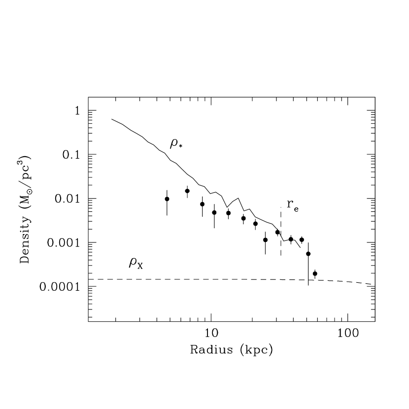
Another way to describe the total cluster population which is more directly relevant to the physical formation efficiency of globular clusters is the mass ratio in the GCS relative to the other halo components (e.g., Harris et al.  (1998); McLaughlin (1999); Kavelaars (1999)). In Figure 4, we explicitly compare the mean mass density profile in the GCS with those of he halo field stars and the hot X-ray gas.

To obtain the three-dimensional density profile of the halo light, we deprojected the halo surface brightness in $\mu_{B}$ (Peletier et al. 1990) in the manner described by McLaughlin (1999) and converted it to mass per unit volume with the assumption $(M/L)_{B}=8$ for an old-halo stellar population (e.g., van der Marel (1991)). The GCS profile was also deprojected with McLaughlin’s algorithm, corrected for clusters fainter than our photometric limit $V=27$ (see below), and multiplied by an assumed mean cluster mass $\langle M_{cl}\rangle=2.5\times 10^{5}M_{\odot}$. In both cases we assumed spherical symmetry to perform the deprojection, along with a surface density profile $\sigma\sim r^{-2}$ at radii beyond our outermost measured annulus (though the shape of the deprojected density profile is not at all sensitive to this latter assumption except for the outermost observed point). Lastly, the X-ray density profile is from Makino (1994, adjusted to a distance scale $H_{0}=70$). Because of its huge radial extent, the gaseous component is at nearly constant density over our region of observation.

To normalize $\rho_{GCS}$ properly to the other components, we divide it by a ratio $\epsilon$ which is the ratio of total mass in the GCS to the total mass in the galaxy within the same radial region, $\epsilon=M_{GCS}/M_{g}$. (The “efficiency” ratio $\eta_{GC}$ used by Blakeslee et al.  (1997) and Blakeslee (1999) can be converted to $\epsilon$ by multiplying it by the mean globular cluster mass $M_{cl}$. We prefer to use $\epsilon$, since it is a strictly dimensionless quantity which can easily be interpreted as the fraction of star-forming mass converted to clusters.) Here, the galaxy mass $M_{g}$ is to be thought of as comprising both the mass in the halo stars and in the X-ray gas, $M_{g}=M_{\star}+M_{X}$, and it implicitly assumes that the gas mass within the region represents either protogalactic material that was unused for star formation, or processed material that was later ejected through supernovae, stellar winds, or tidal stripping. (See the discussions of McLaughlin 1999, Harris et al. 1998, or Blakeslee (1999). In the case of NGC 4874, this assumption may not be correct since the gas is associated with the Coma potential rather than one specific galaxy. However, the distinction is unimportant since $M_{X}$ turns out to be small; see below.)

In essence, $\epsilon$ is then an estimate of the global mass formation efficiency ratio for the globular clusters. To avoid a possible bias in $\epsilon$ from the fact that globular clusters in the inner core of the galaxy will have been preferentially destroyed by dynamical effects (dynamical friction, tidal shocking, and tidally enhanced evaporation), McLaughlin defines this mass ratio for $r\,{}^{>}_{\sim}\,r_{e}$ (the de Vaucouleurs effective radius), outside of which these dynamical effects are small. For NGC 4874, the effective radius is, however, quite large ($r_{e}=66^{\prime\prime}$; Peletier et al. 1990). This restricts us to only the outermost five annuli in our GCS profile and unfortunately leaves only a small overlap with the halo light profile. Nevertheless, under these conditions we find that we need to adopt $\epsilon\simeq 0.003\pm 0.0005$ to bring $\rho_{GCS}$ into alignment with ($\rho_{\star}+\rho_{X}$). In this radial region ($r\,{}^{<}_{\sim}\,55^{\prime\prime}-110^{\prime\prime}$), the halo light contributes 90% of $M_{g}$ and the X-ray gas only 10%.

Our estimate of $\epsilon$ is similar to McLaughlin’s “universal” $\langle\epsilon\rangle=0.0026$ which he derived from the average of M87, NGC 4472, and NGC 1399. Blakeslee (1999) provides additional evidence that $\epsilon$ takes on a similar value in several other brightest-cluster ellipticals. As expected, at smaller radii we see that the GCS profile gradually falls below the halo light. Bearing in mind the uncertainties in the various conversion parameters (particularly the adopted mass-to-light ratios for the clusters and the old-halo light), we therefore suggest that NGC 4874 was roughly as effective at forming globular clusters as were the Virgo and Fornax ellipticals, and other BCG’s.

4 Color and Metallicity Distribution

The final information we need to add to our discussion is the color or metallicity distribution of the GCS. Broad or bimodal MDFs are found in giant E galaxies about half the time (e.g., Kundu & Whitmore (1999)) and are conventionally taken to signal a complex or multi-phase formation history (e.g., Ashman & Zepf (1992); Forbes et al.  (1997); Kissler-Patig et al.  (1998); G.Harris et al.  (1999)). In addition, complex MDFs are certainly more common among the more luminous ellipticals. Here again, however, NGC 4874 turns out to give us a surprise.

Our information about the MDF relies heavily on the relatively small number of clusters with small photometric errors, i.e., those brighter than $V\sim 26$ (although there is no evidence that mean color is correlated in any way with luminosity; see Fig. 2). The distribution of $(V-I)$ with radius $r$ for the brightest objects is displayed in Figure 5. Two results can immediately be drawn from this plot: (a) There is little if any gradient of mean cluster color with radius. (b) The range of colors within the GCS is narrow and relatively blue. All of these results are unexpected to varying degrees. For 146 objects with photometric uncertainties $\sigma(V-I)\leq 0.07$, the mean color is $\langle V-I\rangle=0.907\pm 0.008$, with an rms dispersion $\sigma_{V-I}=0.093$.

In Figure 6, the color distribution is plotted in histogram form, along with a single Gaussian curve with the same mean and standard deviation as given above. A simple Gaussian provides an adequate match to the raw histogram, and clearly we cannot reject the hypothesis that the MDF is unimodal. The average photometric measurement uncertainty is $\pm 0.064$ for this sample; subtracting it in quadrature from the observed width $\sigma_{V-I}=0.093$ then suggests that the intrinsic cluster-to-cluster scatter in color is at the level of $0.06-0.07$ mag.

If we can safely regard the GCS as a conventional “old halo” component (i.e., having formed in the first few Gyr of the galaxy’s history; see below) then the photometric color can readily be translated into metallicity. A new calibration of [Fe/H] against $(V-I)_{0}$ from the Milky Way globular clusters, with data drawn from the 1999 edition of the McMaster catalog (Harris (1996), accessible at http://physun.physics.mcmaster.ca/Globular.html), is shown in Figure 7. A conversion factor $E_{V-I}=1.3E_{B-V}$ is used to deredden the integrated colors. In Fig. 7, solid dots are the integrated colors of clusters with foreground reddenings $E_{B-V}<0.2$, while open symbols are those with $0.2<E_{B-V}<0.6$. Giving more weight to the lower-reddening clusters, we adopt a mean relation

$$(V-I)_{0}=0.17\,{\rm[Fe/H]}\,+\,1.15\,.$$

This relation is slightly steeper than the one derived by Kissler-Patig et al. (1997), namely $(V-I)_{0}=0.15$ [Fe/H] + 1.13, but shallower than an earlier calibration of Couture et al.  (1990), $(V-I)_{0}=0.198$ [Fe/H] + 1.207. Fortunately, the mean color of the NGC 4874 clusters is near the middle of the calibration line, where all of the various conversion relations give similar results.

The sample mean $\langle V-I\rangle=0.907$, with $E_{V-I}$(Coma) = 0.01, gives $\langle$[Fe/H]$\rangle=-1.5\pm 0.05$ (internal uncertainty only). If the external calibration uncertainty of the $(V-I)$ scale is near $\pm 0.05$ (Paper I) then the true uncertainty in this mean metallicity is near $\pm 0.3$ dex. Similarly, the intrinsic color dispersion of $\sim 0.06-0.07$ corresponds to a metallicity histogram width $\sigma$[Fe/H] $\simeq 0.4$. Both the rather low mean metallicity and moderately narrow dispersion strikingly resemble the analogous values for the halo globular clusters in the Milky Way (e.g., Zinn (1985); Harris (1999)) and in dwarf ellipticals (Miller (1999); Harris (1991), 1999). The mean [Fe/H] is also within the range typically occupied by the metal-poor “mode” in giant ellipticals with bimodal MDFs (e.g., Forbes et al.  (1997)). For comparison, we indicate in Fig. 6 the $(V-I)$ colors for the metal-poor and metal-rich halves of the MDFs in M87, NGC 4472, and in several Fornax ellipticals (Whitmore et al.  (1995); Kundu et al.  (1999); Kissler-Patig et al.  (1997); Puzia et al.  (1999)). To within the zero-point uncertainty of our $(V-I)$ color scale (see the cautionary comments below), the lower-metallicity line is similar to the color of the NGC 4874 system. Any metal-rich component is entirely missing, even in the core region.

To turn this very metal-poor MDF into a metal-rich one resembling those found in M87 and other giant E galaxies (at [Fe/H] $\sim-0.5$), we would have to claim that our $(V-I)$ scale zeropoint is wrong by as much as $0.15-0.2$ magnitude, which we regard as extreme. To verify our $(V-I)$ scale, we performed some additional consistency checks. We took measurements of the surface intensity of the NGC 4874 halo light at several locations across the WFPC2 field. The outer edges of the field were used to define background, and the residual light at each location was translated through the photometric calibration equations of Holtzman et al. (1995b; see Paper I) to generate $(V-I)$ integrated colors. The results are shown in Fig. 5 and listed in Table 2. The typical uncertainty of each individual measure is $\pm 0.015$ mag. Although no published measurements for the Coma galaxies in $(V-I)$ are available in the literature for comparison, it is encouraging that our data give $(V-I)\simeq 1.2$ for the core of NGC 4874, which is exactly in the standard range for normal elliptical galaxies (Buta & Williams (1995)).

An additional result of interest on its own merit is the color gradient of the halo, given roughly by $\Delta(V-I)/\Delta({\rm log}r^{\prime\prime})=-0.17$. From Figure 5, we see that the color of the outer halo converges to the mean color of the GCS for $r\,{}^{>}_{\sim}\,100^{\prime\prime}$, suggesting that they have comparably low metallicities there. A gradient of similar nature was also found by Peletier et al.  (1990) in the slightly more metallicity-sensitive index $(B-R)$ (also shown in Fig. 5).

The surface photometry provides a consistency test of the accuracy of the calibration equations, but the stellar photometry of the individual objects involves the additional step of aperture corrections. Faint objects are best measured via PSF fitting or through small apertures, but these must then be normalized to the larger aperture of $0\farcs 5$ radius that is used in the Holtzman et al.  (1995b) transformation equations. The differences between small and large apertures can be estimated through standard curves of growth for the WFPC2 filters (e.g., Holtzman et al. 1995a ; Suchkov & Castertano (1997)). These corrections may differ slightly – typically by a few hundredths of a magnitude – from one CCD to the next on the WFPC2 array, from short to long exposures, and from one filter to another.

In our data reduction, we determined individual empirical PSFs whose instrumental magnitude scales were internally equivalent to an aperture radius $r=0\farcs 2$ (or 2 pixels on the WF2,3,4 fields). We also independently derived aperture corrections from the PSF scale to direct aperture-photometry magnitudes with $0\farcs 2$ radius, and from $0\farcs 2$ to $0\farcs 5$, using isolated stars on each CCD. These adopted corrections are listed in Table 3. Aperture correction values from Holtzman et al. (1995a) and Suchkov & Casertano (1997), obtained from much shorter-exposure standard-star fields, are given for comparison. Although the $V$ offsets in all three studies are similar to within $\pm 0.03$ mag, the discrepancy in $I$ between our work and theirs is larger, by almost 0.1 mag. However, the most important quantity for checking the accuracy of the $(V-I)$ color scale is the difference $\Delta(V-I)$ between the aperture corrections. Here, our average for the WF chips is $\Delta(V-I)=-0.06$, Holtzman et al. give $-0.04$, and Suchkov & Casertano give $+0.025$. Inspection of the relevant tables in their papers indicates that all these values are typically uncertain by $\pm 0.03$ mag, so they are not strongly in disagreement. It is also worth noting that if we had adopted the normalizations of either of these other studies, our $(V-I)$ scale would have been even bluer.

Nevertheless, it would clearly be highly desirable to obtain additional photometry of this system in a color index which is much more sensitive to cluster metallicity than $(V-I)$ and thus more robust against small zeropoint errors: finer structure in the MDF may be revealed, and the metallicity peak can be independently checked.

5 Discussion: Alternatives for Galaxy Formation

The globular cluster system in NGC 4874 presents us with an unanticipated mix of characteristics:

• A “normal” GCLF (that is, a luminosity distribution with Gaussian-like shape in number per unit magnitude, and a turnover luminosity at the expected level for giant ellipticals);

• A spatial distribution with low central concentration and extremely large core radius $r_{c}\simeq 22$ kpc;

• A specific frequency $S_{N}\simeq 4$, very close to the normal value for giant ellipticals that are not cD’s or brightest cluster members;

• A narrow and surprisingly metal-poor metallicity distribution, $\langle$[Fe/H]$\rangle\sim-1.5$ and $\sigma$[Fe/H] $\simeq 0.4$.

As indicated earlier, this combination is unexpected for a cD-type galaxy in particular. The primary goal of this work is to help illuminate the sequence of events during galaxy formation, and we now attempt to fit all of these characteristics into a consistent interpretive picture.

5.1 Defining the Problem

Competing ideas for the formation of E galaxies fall into three basic categories: traditional in situ formation from protogalactic gas; growth by accretion or stripping of neighboring galaxies; and growth by merger of gas-rich disk galaxies with accompanying star formation.

The data for NGC 4874 do not fit easily into any of these standard scenarios. A basic merger-formation or accretion approach might initially seem most attractive for a cD-type galaxy: recent numerical simulations for the way these galaxies build up show that, because of their privileged initial location near the center of a large concentration of pregalactic material, they are likely to undergo a long series of accretions of “fragments” of many different sizes, starting very early in the protogalactic epoch and continuing for several Gyr (e.g., Dubinski (1998); Weil & Hernquist (1996); and references cited there). Such a sequence would seem to provide the richest possible set of opportunities for bringing in both metal-poor and metal-rich halo material, supplies of gas for building new clusters, and growth of the outer halo by harrassment and stripping of small neighbors (Moore et al.  (1996)).

However, the basic problem we encounter in all scenarios for the specific case of NGC 4874 is the lack of metal-rich clusters in the present-day galaxy. For example, the accretion model in the quantitative form given by Côté et al. (1998), or the accretion-by-harrassment variation, assumes that an initial elliptical gains material from smaller neighbors: the original galaxy, which is already moderately large, generates the component of metal-rich clusters and stars during its own single major formation burst, while the metal-poor ones are added later from the smaller cannibalized satellites. The puzzle we face is that in NGC 4874 the metal-rich GCS component is entirely missing, even though the bulk of the galaxy light is clearly red and metal-rich as in normal ellipticals.

In the merger picture (e.g., Ashman & Zepf (1992) and subsequent papers), the metal-poor clusters are assumed to belong to the progenitor disk galaxies while the metal-richer ones are formed from the shocked gas during the merger. (In the sense described by Harris (1999), this process can be thought of as an active merger, while pure accretion is a passive, or gas-free merger in which new stars are not formed.) Since the starlight in the resulting elliptical is predominantly metal-rich, most of its stars should then have formed during the sequence of mergers. Where, then, are the metal-rich clusters that should have formed along with them?

Lastly, the in situ picture supposes that the broad or bimodal MDF characteristic of most gE’s would build up in two major starbursts: the first burst forms the metal-poor clusters and the metal-poor halo field stars, leaving most of the gas unused. Perhaps one or two Gyr later, a second major burst uses up most of the gas and builds most of the metal-rich stars along with the metal-richer clusters (Forbes et al.  (1997); Harris et al.  (1998); G.Harris et al.  (1999)). The metal-poor component in this picture should be more spatially extended, since it is visualized to form while the protogalaxy was still in a clumpy, diffuse state. Here again, we have difficulty understanding the lack of metal-rich clusters, which we would ordinarily have expected to form in the second burst.

5.2 The Metal-Poor Clusters: Normal or Abnormal?

Any interpretation of this unusual galaxy must, at this point, involve a healthy component of speculation. In the spirit of constructing a consistent picture, we suggest that all of the principal anomalies in this galaxy (the narrow and entirely metal-poor MDF; the rather low specific frequency; and the extremely extended spatial distribution) are connected. To put this statement another way, let us pose the following question: what changes would be necessary to make the NGC 4874 GCS resemble the ones that are conventionally regarded as “normal”, such as in the Virgo giants NGC 4472 and M87?

For comparison purposes, let us look more closely at the data for one of the most well studied giant ellipticals, NGC 4472, in which the GCS has a distinctly bimodal MDF and an average $S_{N}\simeq 5$. The excellent photometric study of Lee et al.  (1998) shows unequivocally that the metal-rich (red) and metal-poor (blue) subsystems in NGC 4472 have different spatial distributions. A very similar phenomenon appears to hold in M87 (Lee & Geisler (1993); Kundu et al.  (1999)), though with a larger total cluster population (higher specific frequency). It is therefore interesting to ask whether or not the bluer cluster populations in these comparison galaxies have a characteristic spatial extent (core radius) similar to what we find in NGC 4874.

The breakdown for NGC 4472 is shown in Figure 8. Here the projected density profiles are displayed separately for the metal-poor (blue) and metal-rich (red) populations, along with King-model fits to each. The data for $r>100^{\prime\prime}$ are from Lee et al.  (1998), including clusters brighter than $T_{1}=23$ and with the divisions between the red and blue modes as prescribed in their paper. Data for the inner region $r<100^{\prime\prime}$ are from Harris et al.  (1991), multiplied by a factor 0.7 to correct for their different photometric limit, and multiplied by a further factor of 0.5 with the assumption that there are roughly equal numbers of blue and red clusters in this inner region. For the blue population, we find a core radius $r_{c}\simeq 184^{\prime\prime}$ (or 14 kpc for a distance modulus $(m-M)_{0}=31.0$) and central concentration index $c\simeq 1.2$. For the red population, $r_{c}\simeq 100^{\prime\prime}$ (8 kpc) and $c\simeq 1.0$. The curve fits should be taken only as illustrative of the general shapes of the two subsystems, since the inner regions are not well determined and the outermost background count level is also somewhat uncertain (see Lee et al. 1998). Nevertheless, its low-metallicity cluster population has a radial extent not unlike the GCS in NGC 4874.

In summary, the metal-poor cluster population in NGC 4874 does not appear to be abnormal in total numbers, mean metallicity, or spatial structure by comparison what can be found in other giant ellipticals. The missing metal-rich component is the key to understanding this system. The most obvious single step to convert NGC 4874 into a more normal cD would be simply to add a roughly equal number of metal-rich clusters in the inner part of the galaxy. We would then have a cD galaxy with a bimodal MDF, a comfortably high specific frequency $S_{N}\sim 7$, and a GCS with subcomponents that have distinct spatial distributions as we would normally expect. The one uncomfortable anomaly that we would be left with, of course, would be a higher-than-average mass ratio $\epsilon$. But we do not yet have a comprehensive set of measurements of $\epsilon$, and it remains to be seen whether or not this ratio is a truly universal one.

5.3 Assembling the Metal-Poor Component

An additional and possibly related piece of evidence is that the Coma cluster as a whole appears to have assembled by the merger of smaller subgroups of galaxies. Some of the subcomponents can still be detected in the lumpiness of the X-ray contours on Megaparsec-size scales, and in the redshift and spatial distributions of the galaxies (e.g., Mellier et al.  (1988); Burns et al.  (1994); White et al.  (1993); Biviano et al.  (1996); Secker & Harris (1996); Colless & Dunn (1996); Vikhlinin et al.  (1997); Conselice & Gallagher (1998), among others). The Coma cluster in total is so large, and its two central supergiant galaxies so big, that these supergiants could well have experienced a higher proportion of accretions or mergers than in other giant ellipticals. Such a process, in its entirety, would use a mixture of all three classic galaxy formation scenarios (in situ, accretion, merger): we could plausibly expect that star formation would be taking place vigorously in the dense gas of the central proto-cD at the same time as large gaseous fragments and other partially formed protogalaxies were raining in towards it.

What constraints can be placed on a scenario of this type from only the metal-poor cluster population? It has already been pointed out (see above) that the population of $\sim 9000$ total clusters has an MDF with the same mean metallicity and dispersion as that of a typical halo GCS in a spiral or dwarf galaxy. Possible interpretations for their origin might then be the following:

(a) They formed predominantly in situ during the first round of star and cluster formation in the protogalaxy. In such a view, this epoch must have happened so early that the protogalactic gas was still very clumpy and spatially extended, and nearly unenriched. Its traces are now seen in the low-metallicity cluster population with its extremely large core radius, but not in the main bulk of the galaxy (which is dominated by a redder, much more metal-rich and more centrally concentrated stellar population). Accretion and stripping from small satellites might have added more clusters and some metal-poor light later on, building up the outer halo as it is seen today.

(b) They formed predominantly in smaller, metal-poor galaxies which were then accreted by NGC 4874. Many accretions must have been involved, combining a wide mixture of dwarfs and disk-type galaxies more or less in the manner employed in the model by Côté et al. (1998).

Let us explore this latter approach in a bit more detail. The near-complete lack of clusters more metal-rich than about [Fe/H] $\simeq-0.5$ ($V-I=1.1$) suggests that not much accreted material came from other fully formed giant elliptical galaxies, since these would almost certainly have added metal-rich globulars to the GCS, which is contrary to what we observe. More quantitatively, we can ask how many clusters might have been accumulated from smaller galaxies without leading to contradictions in either the GCS metallicities or the (red) integrated color of the halo light.

Published analyses of the dE galaxies in Coma show that the fainter dE’s are depleted in the core relative to the brighter dE’s and giant ellipticals (Lobo et al.  (1997); Secker et al.  (1997); Thompson & Gregory (1993); Bernstein et al.  (1995); Trentham (1998)). The effect is most strongly evident for dwarfs in the magnitude range $19\,{}^{<}_{\sim}\,R\,{}^{<}_{\sim}\,22.5$ (or $-15.4\,{}^{<}_{\sim}\,M_{V}\,{}^{<}_{\sim}\,-11.9$, assuming $(V-R)=0.6$ for a typical dE). These intermediate-luminosity dE’s have a nearly flat projected density distribution in the Coma core ($r\,{}^{<}_{\sim}\,10^{\prime}$), whereas the bright Coma ellipticals follow a steeper distribution distribution $\sigma\sim r^{-1}$ closer in to the center (Bernstein et al.  (1995); Trentham (1998)). Interestingly, the faintest dE’s ($R\,{}^{>}_{\sim}\,22.5$) appear to show a centrally concentrated radial distribution more like the giants (Bernstein et al.  (1995)). In addition, the luminosity function of the dE’s may be somewhat steeper in the outer regions of Coma than in the core, suggesting again that depletion has occurred in the core (Lobo et al.  (1997); but see Trentham (1998)).

From the radial profile data of Secker et al. (1997) and Bernstein et al. (1995), we find that adding in about 850 dE’s in the faint range $19<R<23$ within $r<8^{\prime}$ (250 kpc) would be sufficient to bring their radial distribution back up to the fiducial $\sigma(r)\sim r^{-1}$ characterized by the brighter ellipticals. This number is about 1.5 times the present-day population of faint dE’s in the same region. The slightly brighter dE’s ($R<19$) also exhibit a flat distribution $\sigma\sim r^{-0.5}$, though less so than does the faintest group. Increasing their numbers by $\sim 50-75$ (or 50 to 100 percent of their present-day core population) would bring them back to the fiducial $r^{-1}$ profile as well. In short, it seems plausible to suggest from the radial distribution data that roughly 1000 small galaxies may have been removed from the Coma core region.

For purposes of building a strawman argument, let us now assume that these “missing” galaxies were indeed present at earlier times but were absorbed by the central supergiant. We can then assess how they would have affected its globular cluster system and halo light. In the same manner as Côté et al. (1998), we perform a numerical experiment in which these effects are built in:

• We assume, as above, that 1000 galaxies are accreted, and that they follow the composite luminosity distribution shape given by Secker & Harris (1996). The normal ellipticals follow a Gaussian number distribution peaked at $R=14.5$ with dispersion $\sigma(R)=0.80$, while the dwarf ellipticals follow a Schechter function with $R^{\star}=15.6$ and power-law slope $\alpha=-1.4$.

• We assume that all the galaxies have a “normal” specific frequency $S_{N}=4$ (Durrell et al.  (1996); Miller et al.  (1998); Harris et al.  (1998)), which fixes their total contribution to the globular cluster population once the luminosity is specified.

• We assume that the integrated color (i.e., metallicity) of each galaxy increases with its luminosity according to the observed correlation for Coma dwarfs (Secker et al.  (1997)), $(B-R)=2.41-0.056R$. The $(B-R)$ index can be converted to $(V-I)$ through $(V-I)_{0}\simeq 0.58(B-R)_{0}+0.24$, valid for the Milky Way globular clusters.

• Finally, we assume that the mean metallicity of the globular clusters in each dwarf is correlated with galaxy luminosity according to the relation derived by Côté et al. (1998), [Fe/H] $=2.31+0.638M_{V}+0.0247(M_{V})^{2}$. Although bigger and brighter galaxies have more metal-rich clusters on average, the mean [Fe/H] is only a weak function of $M_{V}$ for the majority of the dwarfs (see also Forbes et al.  (1997)). In addition, the average metallicity of the clusters is lower than that of the galaxy they are in by typically $\sim 0.5$ dex (Miller (1999)). Thus, the combined galaxies can have a rather metal-poor GCS while their aggregated halo light is somewhat more metal-rich.

The final parameter we employ is $M_{V}$(max), the upper cutoff to the LF (that is, the luminosity of the brightest accreted galaxy). In summary, our numerical procedure is to assume a value for $M_{V}$(max), and add together 1000 galaxies fainter than this limit which are distributed according to the rules listed above. We then ask how many globular clusters these would contribute, what their mean metallicity will be, and what color the combined halo light will have. Larger accreted galaxies are rarer, but have more populous GCSs and redder (more metal-rich) clusters and halo light.

The results of this numerical exercise are summarized in Figure 9 as a function of the upper cutoff $M_{V}$(max). (Rather similar information is contained in the more extensive Monte Carlo models discussed by Côté et al.  (1998); see especially their Figures 6 and 7). The most important single trend to note is that all the output quantities (the number of accreted clusters $N_{cl}$, their mean [Fe/H], and the mean halo color $(V-I)$) are strongly sensitive to how many bright galaxies are in the sample. Although the luminous galaxies are individually rare, each one contributes so much total material that they tend to dominate the integrated sums.

These results can be used to place rough limits on the degree of accretion that NGC 4874 has experienced. It is unlikely that many galaxies more luminous than $M_{V}\sim-19$ have been accreted, since these would drive the mean GCS metallicity to unacceptably high levels (the actual MDF is indicated on the right side of the lower panel). At nearly this same $M_{V}$(max), we would also run into trouble with the total number of accreted clusters, which would approach the permitted maximum of $\sim 9000$. However, if we stay within the allowed margin $M_{V}$(max) $\,{}^{>}_{\sim}\,-19$ to $-18$, the color of the halo light contributed by the accreted objects stays within $(V-I)\simeq 1.0\pm 0.1$. It is an important consistency test that this color range is comfortably within the observed range for the outer halo of NGC 4874 (Fig. 5).

In summary, the accretion model yields a fairly broad range of possibilities which would fit within the observational constraints that we have. With the assumptions as listed above, we would suggest that as much as half of the total cluster population could have originated by accretion. Such a model would simultaneously be consistent with (a) the MDF of the clusters as we see it today, (b) the extended radial distribution of the GCS, (c) the color of the outer-halo light, and (d) the present-day depletion of the dE’s in the central Coma region.

The first-order model we have just described does not, by any means, lay out the full range of possibilities that could be explored in more extensive simulations. (For example, the Schechter LF exponent for the input dE’s could be varied, as could their specific frequencies. Both of these parameters would be capable of generating noticeable differences around the mean lines shown in Fig. 9.) It is precisely this range of possibilities which makes it difficult to answer just how much of the galaxy is accreted material, as opposed to stars converted from in situ gas. Because most galaxies of all types – dwarf ellipticals, irregulars, spirals, and giant ellipticals – contain a subpopulation of metal-poor globular clusters ([Fe/H] $\sim-1.6$ to $-1.0$) with only a weak dependence on galaxy size, we cannot easily tell where such clusters might have come from, except to rule out very luminous parents.

5.4 The Strange Case of the Missing Red Clusters

The foregoing arguments lead us to conclude that accretion of smaller satellites may have played an important role in the history of this Coma supergiant. But the accretion (passive-merger) model cannot explain the presence of the much redder, more metal-rich material ($(V-I)\simeq 1.2$; see Fig. 5) in the central $\sim 20$ kpc of NGC 4874 which dominates its total light. For this, we need to resort either to in situ second-generation star formation or to very gas-rich mergers which would be capable of driving the mean metallicity up to its observed high levels. Star clusters probably also formed during this stage as part of the general conversion of gas into stars, since star clusters are found almost universally in star-forming regions (e.g., Elmegreen et al.  (1999)). Why are none of those clusters visible today? To avoid appearing in our photometric survey, any such objects would have to be fainter than $V\sim 28$, or less massive than about $10^{5}M_{\odot}$ for a normal globular cluster age.

The formation of massive, globular-sized clusters ($10^{5}-10^{6}M_{\odot}$) is likely to require local reservoirs of gas in the range of $\sim 10^{8}M_{\odot}$ or more (Searle-Zinn fragments or supergiant molecular clouds; e.g., Searle & Zinn (1978); Larson (1993); Harris & Pudritz (1994)). By implication, giant molecular clouds (GMCs) this large may therefore not have been present in NGC 4874 during the stage when most of the galaxy was being assembled. If, during this main star-forming stage, NGC 4874 was simultaneously experiencing a wide range of tidal shocking, gas infall, merging, supernova shocks, and internal winds, then the supergiant GMCs that would normally make up the protogalaxy might have been extensively broken down into smaller fragments. With this line of reasoning, we would have to postulate either that these processes were more violent for NGC 4874 than in M87 or other giant ellipticals with metal-rich clusters; or, that the timing of these events was such that they were particularly effective at disrupting the large gaseous fragments. Then, almost all the star formation took place within these smaller GMCs.

An evolutionary picture along these lines would imply that metal-rich star clusters did form along with the main bulk of the galaxy, but that they were in a mass range $\,{}^{<}_{\sim}\,10^{5}M_{\odot}$ which would fall below the limits of our photometric survey. We can further speculate that these smaller star clusters – more easily subject to dynamical destruction than the massive ones – have to a large extent already dissolved into the general field, leaving few traces in the GCS that we see today.

An additional observation which is, perhaps, consistent with a such a view is that the active mergers between disk galaxies which we can directly observe today (e.g., Zepf et al.  (1999); Whitmore & Schweizer (1995); Whitmore et al.  (1999)) seem to be efficient at producing large numbers of low-mass star clusters. (For example, the well known Antennae merger has generated well over 1000 low-mass ($M\,{}^{<}_{\sim}\,10^{5}M_{\odot}$) clusters but only a few dozen massive young globulars.) For this reason, these same mergers will generate ellipticals with rather modest specific frequencies in the range $S_{N}\sim 2-3$ (Harris (1999) and the papers listed above), since it is the high-mass clusters which survive longest and determine the long-term value of $S_{N}$.

It is obvious that the storyline we have just proposed has strong elements of “special pleading”; that is, arguments constructed specifically for one situation. But NGC 4874 presents us with a unique and outstanding set of GCS features within a rare type of galaxy, and we may in the end be forced to deal with it in a different way than with more normal ellipticals.

6 Summary

HST/WFPC2 photometry in $V$ and $I$ has been obtained for the globular cluster system in NGC 4874, the central cD in Coma. The luminosity function (GCLF) of the clusters has the normal Gaussian-like shape and turnover level, but several other features of the system prove to be surprising. The GCS is spatially very extended, with core radius $r_{c}\sim 22$ kpc, and the metallicity distribution function is unimodal, narrow ($\sigma$[Fe/H] $\simeq 0.4$), and entirely metal-poor ($\langle$[Fe/H]$\rangle\sim-1.5$). Lastly, the total population $N_{t}\simeq 9000\pm 1000$ gives a specific frequency $S_{N}=3.7\pm 0.5$ which is in the typical range for normal ellipticals but strikingly low for central cD-type galaxies.

We suggest that the principal anomaly in this GCS is essentially the complete lack of metal-rich clusters. If these were present in normal (M87-like) numbers in addition to the metal-poor ones that are already there, then the GCS in total would closely resemble what we see in many other dominant cD galaxies. This supergiant galaxy, in its early stages, appears to have avoided forming globular clusters during the main metal-rich stage of star formation which built the bulk of the galaxy. This situation presents strong challenges to all three of the classic modes of galaxy formation: accretion, disk mergers, and in situ formation. As a best-compromise interpretation, we suggest that up to half the cluster population could have been gained by the accretion of small satellite galaxies which richly populated the Coma core region at earlier times. But the main, metal-rich star formation stage which built the inner parts of the galaxy must have somehow avoided generating massive star clusters. We suggest that massive high-metallicity globulars did not form because the normal sites of globular cluster formation – supergiant molecular clouds – had already been broken down into smaller clouds at the time the metal-rich star formation was taking place.

Table 1: GCS Radial Profile Data

$r$	n	Area	$\sigma$	$\rho$
(arcsec)		(arcsec2)	(arcsec-2)	($M_{\odot}$ kpc-3)
9.9	$86.86\pm 9.94$	236.06	$0.3680\pm 0.0421$	25800
13.6	$82.46\pm 9.70$	236.55	$0.3486\pm 0.0410$	39400
17.9	$60.06\pm 8.31$	212.65	$0.2824\pm 0.0391$	19700
19.3	$94.64\pm 10.44$	368.27	$0.2570\pm 0.0283$	12700
27.6	$133.16\pm 12.34$	558.76	$0.2383\pm 0.0221$	12400
35.5	$163.34\pm 13.64$	798.82	$0.2045\pm 0.0171$	9350
43.4	$169.79\pm 13.93$	981.35	$0.1730\pm 0.0142$	7090
51.2	$187.49\pm 14.57$	1254.53	$0.1494\pm 0.0116$	3040
55.2	$402.11\pm 21.39$	2811.67	$0.1430\pm 0.0076$	4540
70.3	$388.91\pm 21.04$	3396.13	$0.1145\pm 0.0062$	3140
85.7	$298.71\pm 18.47$	3263.40	$0.0915\pm 0.0057$	3070
100.0	$107.63\pm 11.08$	1739.88	$0.0619\pm 0.0064$	1470
119.1	$25.95\pm 5.40$	496.25	$0.0523\pm 0.0109$	520

Table 2: Surface Photometry for NGC 4874

$r$ (′′)	$(V-I)$	$r$ (′′)	$(V-I)$
1.33	1.289	9.65	1.225
2.79	1.290	16.52	1.213
2.92	1.303	17.97	1.192
2.99	1.298	19.25	1.215
3.23	1.289	22.00	1.180
3.43	1.287	27.00	1.180
3.96	1.268	32.00	1.155
4.18	1.265	35.00	1.130
4.53	1.285	60.00	1.080
5.24	1.247	95.00	0.930
7.51	1.227

Table 3: Aperture Corrections for Photometric Calibration

Source	$\Delta V$ (WF)	$\Delta I$ (WF)	$\Delta V$ (PC1)	$\Delta I$ (PC1)
This study	0.25	0.31	0.24	0.31
Holtzman et al. 1995a	0.19	0.23	0.20	0.23
Suchkov & Casertano 1997	0.23	0.21

Figure 1: Plot of the brighter starlike objects ($V<27.0$) detected and measured in the NGC 4874 WFPC2 field. The galaxy center is at $(59^{\prime\prime},95^{\prime\prime})$ near the center of the PC1 chip. Cardinal directions (north, east) relative to the center of NGC 4874 are marked with the straight lines. Objects regarded as “nonstellar” according to image structure analysis (see Paper I) have been culled from the sample. The area nearest the center of NGC 4874, and three neighboring E galaxies marked with the circles (NGC 4871, 4872, 4873) were masked out in the analysis, as were narrow areas of slight vignetting along the four chip edges.

Figure 2: Color-magnitude diagram for all starlike objects in the NGC 4874 field with measured $(V-I)$ color indices. The $I-$band exposures were significantly shorter than $V$, so that the data for $I\,{}^{>}_{\sim}\,25$ are very uncertain.

Figure 3: Radial profile for various components of the NGC 4874 system. Solid dots with error bars: the profile for the globular cluster system (from Table 1, with $\sigma_{cl}=\sigma-\sigma_{b}$ and an adopted background level $\sigma_{b}=0.02$ arcsec^-2). Open circles show the outermost five annuli as they would be if the background density was arbitrarily assumed to be zero. Solid line: halo light profile in the $R-$band, from Peletier et al. (1990). Dashed line: halo light profile in the Gunn $r-$band, from Jorgensen et al. (1992). Dotted line: surface intensity $S_{X}$ of the intracluster X-ray halo gas in the Coma cluster (see text). The light and X-ray profiles have been arbitrarily shifted vertically for display purposes; see the next figure for a comparison with proper normalization.

Figure 4: Volume density profiles for three components of the NGC 4874: the halo light (solid line, labelled $\rho_{\star}$), the globular cluster system (solid dots), and the X-ray halo gas (dashed line, labelled $\rho_{X}$). The globular cluster density profile has been divided by a mass ratio $\epsilon=M_{GCS}/M_{g}=0.003$ to normalize it to the halo light; see text for discussion. The effective radius of the galaxy light, $r_{e}\simeq 66^{\prime\prime}\simeq 32$ kpc (Peletier et al.1990) is marked.

Figure 5: Color index $(V-I)$ versus radius for the brightest globular clusters in NGC 4874 ($V\leq 25.5$). Upper solid line: Color profile in $(B-R)$ for the halo light of NGC 4874, from Peletier et al.(1990). Lower solid line: Our measurement of the $(V-I)$ halo color; see text.

Figure 6: Distribution in $(V-I)$ of the brightest clusters in NGC 4874. A total of 146 objects with photometric uncertainty $\sigma_{V-I}\leq 0.07$ are shown, as a histogram of number per 0.05-mag bin. Dashed line: Gaussian curve with mean $(V-I)=0.907$ and standard deviation $\sigma=0.093$, the same as the raw histogram. Vertical dotted lines: The lines at $(V-I)=0.95$ and 1.20 represent the approximate locations of the two modes found in M87 and other Virgo and Fornax galaxies; see text.

Figure 7: Calibration of $(V-I)$ color index against metallicity [Fe/H] for the Milky Way globular clusters.

Figure 8: Radial distribution for the globular cluster populations in the Virgo elliptical NGC 4472. Projected surface density (number of clusters per arcmin²) is plotted against mean radius $r$(arcsec) for several annuli covering the range $r\simeq 2.3-40$ kpc. Solid symbols are the metal-rich (redder) clusters, open symbols the metal-poor (bluer) clusters. Data are taken from Lee et al. (1998), except for the small triangles at upper left, which are from Harris et al. (1991). The lines superimposed on each component are King-model fits with parameters as given in the text.

Figure 9: Numerical model for an accreted globular cluster population. Here it is assumed that NGC 4874 has accreted 1000 galaxies fainter than $M_{V}$(max) which follow the Schechter-like luminosity function given in the text. The upper panel shows the total number $N_{cl}$ of accreted globular clusters from these galaxies, assuming that they all have a normal specific frequency $S_{N}=4$. In the lower panel, the solid line shows the mean [Fe/H] for the accreted clusters, with the observed metallicity range of the NGC 4874 clusters shown by the large error bar at right. The dashed line shows the mean $(V-I)$ color of the accreted halo light.