Sub-Arcsecond Imaging of 3C 123:
108-GHz Continuum Observations of the Radio Hotspots
Abstract
We present the results of sub-arcsecond 108 GHz continuum interferometric observations toward the radio luminous galaxy 3C 123. Using multi-array observations, we utilize the high u,v dynamic range of the BIMA millimeter array to sample fully spatial scales ranging from 05 to 50. This allows us to make one-to-one comparisons of millimeter-wavelength emission in the radio lobes and hotspots to VLA centimeter observations at 1.4, 4.9, 8.4, and 15 GHz. At 108 GHz, the bright, eastern double hotspot in the southern lobe is resolved. This is only the second time that a multiple hotspot region has been resolved in the millimeter regime. We model the synchrotron spectra of the hotspots and radio lobes using simple broken power-law models with high energy cutoffs, and discuss the hotspot spectra and their implications for models of multiple hotspot formation.
1 Introduction
Hotspots in the jets of radio galaxies are manifestations of the interaction between the jet and the intergalactic medium— a strong shock which converts some of the beam energy into relativistic particles (Blandford & Rees 1974). Morphologically, hotspots are bright compact regions toward the end of the jet lobe, primarily observed in the radio with a few sources having optical counterparts (e.g. Läteenmäki & Valtaoja 1999). First detected in Cygnus A (Hargrave & Ryle 1974), hotspots are a characteristic and ubiquitous feature in high luminosity, class FRII radio galaxies (Fanaroff & Riley 1974) that can provide constraints on the energetics of the lobes and the powering of radio loud active galactic nuclei.
Unfortunately, the simple, constant beam model of Blandford & Rees does not fully explain the common occurrence of multiple hotspot regions in radio galaxies and quasars (cf. Laing 1989). To accommodate these observations, two modifications have been proposed: (1) the end of the beam precesses from point to point, the ‘dentist’s drill’ model of Scheuer (1982) or (2) the shocked material flows from the initial impact site to the secondary site, the ‘splatter-spot’ model of Williams & Gull (1985) or the deflection model of Lonsdale & Barthel (1986). Both of these models predict that there should be a compact hotspot at the jet termination; indeed, observations have shown that when the jet is explicitly seen to terminate, it is always at the most compact hotspot (Laing 1989; Leahy et al. 1997; Hardcastle et al. 1997).
However, the models in their simplest forms predict two essentially different physical processes in the hotspots. If the secondary (or less compact) hotspots are the relics of primary (more compact) hotspots, as suggested in the ‘dentist’s drill’ model, then the shock-driven particle acceleration has ceased, and the spectrum of the continuum emission seen toward these objects will steepen rapidly with increasing frequency as a result of synchrotron aging and adiabatic expansion. On the other hand, the secondary hotspots in the ‘splatter-spot’ or deflection models still have ongoing particle acceleration as a result of outflow from the primary hotspot, and as long as the observing frequency does not correspond to an energy close to the expected high-energy cutoff in the electron population, the spectral index will not be steeper than = 1.0 (where S ), indicative of a balance between spectral aging and particle acceleration. Of course, it may be that neither of these simple models can properly describe the physics of the interaction. For example, in a more sophisticated version of the dentist’s drill model (Cox, Gull, & Scheuer 1991), the disconnected jet material can continue to flow into the secondary hotspot, causing particle acceleration for some time after the disconnection event. This type of hybrid model will make predictions that will not always be distinguishable from the simple cases.
Hotspots have been well studied with high resolution at radio frequencies. To probe the hotspot regions at higher electron energies, and test models for multiple hotspot formation, we present, in this paper, the first high-resolution image of the FRII radio galaxy 3C 123 in the 108 GHz continuum, focusing on the hotspot regions. The radio galaxy 3C 123 (z = 0.218; Spinrad et al. 1985) is one of the original FRII objects from Fanaroff & Riley (1974) and has an extremely high radio luminosity, a highly unusual radio structure (Riley & Pooley 1978), and an optically peculiar host galaxy (Hutchings 1987; Hutchings, Johnson & Pyke 1988). With the highest resolution to date at these high frequencies, we can compare the morphology and emission of the hotspots to other high-resolution images at longer wavelengths.
Throughout the paper we use a cosmology with km s-1 Mpc-1 and . With this cosmology, 1 arcsecond at the distance of 3C 123 corresponds to 4.74 kpc. The physical conditions we derive in the components of 3C 123 are not sensitive to the value of .
2 Observations and Imaging
3C 123 was observed in three configurations (C, B, and A) of the 9-element BIMA Array111The BIMA Array is operated by the Berkeley Illinois Maryland Association under funding from the National Science Foundation. (Welch et al. 1996). The observations were acquired from 1996 November to 1997 February, with the digital correlator configured with two 700 MHz bands centered at 106.04 GHz and 109.45 GHz. The two continuum bands were checked for consistency, then combined in the final images. During all of the observations, the system temperatures ranged from 150-700 K (SSB).
In the compact C array (typical synthesized beam of 8), the shortest baselines were limited by the antenna size of 6.1 m, yielding a minimum projected baseline of 2.1 k and good sensitivity to structures as large as 50. This resolution is critical for obtaining an accurate observation of the structure in the large-scale radio-lobes. In the mid-sized B array (typical synthesized beam of ), the observations are sensitive to structures as large as . In the long-baseline A array (typical synthesized beam of ), the longest baselines were typically 450 k. With the high-resolution imaging of the hotspots, we can make direct comparisons of the hotspots, and their components, out to millimeter wavelengths. The combination of the three arrays provide a well sampled u,v plane from 2.1 k to 400 k.
The uncertainty in the amplitude calibration is estimated to be between 10% and 15%. In the B and C arrays, the amplitude calibration was boot-strapped from Mars. In the A Array, amplitude calibration was done by assuming the flux density of the quasar 3C 273 to be 23.0 Jy. This flux assumption was an interpolation through the A array configuration and supported by data from other observatories. Absolute positions in our image have uncertainty due to the uncertainty in the antenna locations and the statistical variation from the signal-to-noise of the observation. These two factors add in quadrature to give a typical absolute positional uncertainty of 10 in the highest resolution image.
The A array observations required careful phase calibration. On long baselines, the interferometer phase is very sensitive to atmospheric fluctuations. We employed rapid phase referencing; the observations were switched between source and phase calibrator (separation of 9) on a two minute cycle, to follow the atmospheric phase (Holdaway & Owen 1995; Looney, Mundy, & Welch 1997). Since 3C 123 was one of three sources included in the A array calibration cycle, the time spent on-source was approximately 3 hours; thus, the noise in the high-resolution image is higher than would otherwise be expected in a single track with the BIMA array.
3 Results
The data span u,v distances from 2.1k to 430k, providing information on the brightness distribution on spatial scales from 04 to 60. In order to display the complete u,v information in the image plane, we imaged the emission with four different u,v weighting schemes which include all of the u,v data and stress structures on spatial scales of roughly 5, 3, 1, and 0. These resolutions were obtained with natural weighting, robust weighting (Briggs 1995) of 1.0, robust weighting of -0.2, and robust weighting of -0.6, respectively. All data reduction was performed using MIRIAD (Sault, Teuben, & Wright 1995), and the images shown were deconvolved using the CLEAN algorithm (Högbom 1974).
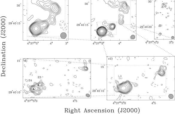
The 108 GHz continuum emission from 3C 123, imaged at the four resolutions mentioned above, is shown in Fig. 1. In this Figure, each successive panel is a higher-resolution zoom, beginning with the 5 image. Fig. 1a shows the large-scale overall jet-lobe structure, which is very similar to lower frequency images (e.g. Hardcastle et al. 1997) and other low resolution millimeter images at 98 GHz (Okayasu, Ishiguro, & Tabara 1992). Our observations, which have more sensitivity to large-scale structure and better signal-to-noise than the 98 GHz data, do not detect the extended emission to the south of the bright eastern hotspot that is seen at longer wavelengths (component F of Riley & Pooley 1978). We also do not detect feature H of Okayasu et al. (1992), which does not in any case correspond to any feature seen on lower-frequency radio images.
In Fig. 1b, the 4 major sources of millimeter emission at 3 resolution are clearly distinguished– from east to west, the eastern hotspot, the core, the western hotspot, and the northwest lobe, respectively. As the resolution increases to 1 in Fig. 1c1 and 1c2, the western hotspot and the northwest lobe corner are resolved into three peaks that contain only a small fraction of the large scale flux. Since the interferometer is acting as a spatial filter, this implies that the northern lobe consists mainly of large-scale emission; however, the eastern hotspot is dominated by compact emission at this resolution. In the highest resolution image, Fig. 1d, the eastern hotspot is resolved at a principal axis of 38, while the core is a point source. The western hotspot is too faint to be seen in this image. Our image of the eastern hotspot looks very similar to high resolution 8.4 GHz observations (Hardcastle et al. 1997), which resolve the hotspot into two components — an extended southeastern component (E4), which corresponds to the peak of the 108 GHz image, and a very compact northwestern component (E3), which accounts for the extension seen in the present image.
4 VLA data and Spectral Indices
To compare our data with observations at longer wavelengths, we obtained existing Very Large Array (VLA) data or images at 1.4, 5, 8.4 and 15 GHz. The 1.4 GHz image was taken from Leahy, Bridle & Strom (1998) based on observations with the VLA A configuration, the 5 and 15 GHz were re-reduced observations by R. A. Laing from the VLA archive using A and B configurations and B and C configurations respectively, and the 8.4 GHz data were from Hardcastle et al. (1997), using A, B and C configurations. All these datasets have shortest baselines very similar to that of our BIMA data, so that they sample comparable largest angular scales; with the exception of the 1.4 GHz data, they are also comparable in longest baseline and thus angular resolution. Flux density scales were calibrated using observations of 3C 48 and 3C 286; we applied a correction to the flux levels of the 15 GHz B-configuration data to compensate for an estimated 7% decrease in the flux density of 3C 48 between the epoch of observation (1982 August 06) and the epoch at which the flux density coefficients for 3C 48 used in AIPS were measured (1995.2).
Having imaged the VLA data, we measured the flux densities of the various components of 3C 123 using the regions specified on the 8.4 GHz VLA image in Fig. 2. These flux densities are tabulated in Table 1. Except where otherwise stated in the final column of the Table, they are derived by integration using MIRIAD, from aligned images, convolved to the same (3) resolution, with polygonal regions defined on low-frequency images. This process ensures that we are measuring the same region at each frequency. The exceptions are the flux density of the core, which was measured by fitting a Gaussian to the matched-resolution maps, and the flux densities of the two components of the E hotspot, which were measured from maps with resolution matched to the highest resolution of the BIMA data. Using these flux densities, we derived a spectral index between each of the 5 frequencies (4 two-point spectral indices). Table 2 lists these spectral indices for each component in the four bands.
The radio core shows an approximately flat spectral index across the radio and millimeter bands. The 8.4 GHz data were taken in 1993–1995 while the other radio frequencies were taken in 1982–1983, so we are comparing data separated in time by a decade, but there was no evidence for core variability on timescales of years in the observations at different epochs that make up the 5, 8.4 and 15 GHz datasets, and the similarity in the flux densities at 8.4 GHz and 5 and 15 GHz [cf. also the 15 GHz core flux density of 120 mJy from Riley & Pooley (1978) and the 5 GHz core flux density of 99 mJy measured from the MERLIN images of Hardcastle et al. (1997)] suggests that there is little variability even on timescales of decades at centimeter wavelengths, contrasting with the variability found in some other well-observed radio galaxies with bright radio cores. However, our 108 GHz core flux density is a factor 3 lower than the flux density measured by Okayasu et al. (1992) between 1989 and 1990 at 98 GHz. Either the spectrum cuts off very sharply between these frequencies — more sharply than would be expected in a synchrotron model — or, more probably, the core is more variable at higher frequency. It is generally found in studies of core-dominated objects that the amplitude of nuclear variability is higher in the millimeter band than at centimeter wavelengths, a fact which can be explained in terms of synchrotron self-absorption effects at lower frequencies (e.g., Hughes, Aller & Aller 1989). Unfortunately, little is known about the millimeter-wave variability of lobe-dominated objects like 3C 123.
All the other components of the radio source have relatively steep spectra even at centimeter wavelengths. As expected, the flattest spectra are observed in the hot spots. We cannot distinguish between the NW and SE component of the E hotspot, within the errors, on the basis of their high-frequency spectral indices, and the W hotspot, also detected at 108 GHz, has a comparable spectrum. The southern lobe (all extended emission to the south of the eastern hotspot, see Fig. 2) has spectral indices which indicate a spectral cutoff at centimeter wavelengths, so it is not surprising that we do not detect it at 108 GHz. However, the northern lobe (the extended emission E and S of the ‘NW corner’) shows no strong indication of a spectral cutoff even at millimeter wavelengths.
5 Spectral Fitting
In order to investigate the synchrotron emission, we fit simulated spectra to the different components of the source, using the code from Hardcastle, Birkinshaw & Worrall (1998). We assume an injection energy index for the electrons of 2, corresponding to a low-frequency spectral index of 0.5, since we cannot derive an injection index from any of our existing data; the 81.5 MHz scintillation measurements of Readhead & Hewish (1974) suggest a flatter spectral index for the hotspots, but this low frequency may be below a spectral turnover due to synchrotron self-absorption or a low-energy cutoff in the electron energy spectrum, as seen in the hotspots of Cygnus A (Carilli et al. 1991). To find magnetic field strengths, we assume equipartition between the electrons and magnetic fields, with no contribution to the energy density from relativistic protons. The choice of an equipartition field does not affect our conclusions about spectral shape, but does affect our estimates of break and cutoff electron energies. Since the fitting is essentially done in the frequency domain, all energies quoted may be scaled by a factor if the field deviates from equipartition. We perform fitting of the simulated spectra by combining the systematic errors in flux calibration (fixed at 2% for the VLA data and 10% for the BIMA data) with the statistical errors tabulated in Table 1; the systematic errors are the dominant source of error for the VLA data. Because the systematic errors are uncorrelated from frequency to frequency, this procedure is valid when fitting spectra, though not when comparing fluxes or spectral indices from different parts of the source.
We consider two basic models for the electron energy spectrum. Both have high-energy cutoffs, but one has a constant electron energy index of 2, while the other is a broken power law model, allowed to steepen from an electron energy index of 2 to 3 at a given energy. The latter is appropriate for a situation in which particle acceleration is being balanced by synchrotron losses or in which loss processes are important within the hotspot (Pacholczyk 1970; Heavens & Meisenheimer 1987). These two models are equivalent to models (i) and (ii) of Meisenheimer et al. (1989), respectively.
5.1 Component Fitting Results
The fitting results are tabulated in Table 3. We find that model (i), the simple, single power-law, never fits the data well, and that in half of the component fits, model (ii), the broken power-law model, fits well with a very high-energy cutoff (labeled as “break” in Table 3). For the rest of the components, a broken-power law and a high-energy cutoff within our data’s frequency range is necessary (labeled as “both” in Table 3). For the chosen model, we tabulate the equipartition magnetic field strength in nT and the best-fitting break energies and, where appropriate, cutoff energies in GeV.
The NW component of the E hotspot (E3) is well fit with the break model (Fig. 3a), but it is very poorly fit with break models having a energy cutoff within our data frequency range; all of the best high cutoff fits to our data have cutoff energies above eV (corresponding to GHz). This is due mainly to the essentially constant spectral index between 8 and 108 GHz. The SE component of the E hotspot (E4) is also best fit with a broken power-law spectrum, although not as well, and only poorly with a high-energy cutoff spectrum (Fig. 3b).
These results differ from the conclusion of Meisenheimer, Yates & Röser (1997), who prefer a model with only a high-energy cutoff as a fit to the overall spectrum of the eastern hotspot. This may be the result of subtle measurement differences in the regions and frequencies used by Meisenheimer et al., who took flux densities for the E hotspot from a variety of sources in the literature, or it may be the effect of combining the two hotspot regions. Our results are more consistent with the model favored by Meisenheimer et al. (1989).
The W hotspot is also best fit with a broken power-law model (Fig. 3c), although no fit is particularly good because of the anomalously flattening spectral index between 15 and 108 GHz that our simple models cannot reproduce. The effect may be due to a bad data point at 15 GHz, but it should be noted that we are not resolving the two components of this hotspot (Hardcastle et al. 1997), so the spectral situation is probably more complex than is represented by our simple one-component model. Again, a high-energy cutoff within our frequency range fits the data even more poorly.
Although the northwest corner region is resolved out at high resolution, it dominates the western side of our low-resolution 108 GHz images (Fig. 1a). The spectrum of this region is smoothly curved from centimeter to millimeter wavelengths. It is poorly fit with a single power-law and cutoff model, but reasonably well fit with a spectral break model; however, better fits are obtained with a model with a high-energy cutoff as well as a spectral break (though the improvement is not significant on an F-test) because of the steep 15–108 GHz spectral index.
The northern lobe’s spectrum is poorly fit with the break model or with a high-frequency cutoff; even the combination of the two, though a substantial improvement, gives a clearly poor fit, modeling the 108 GHz data badly (Fig. 3d), because of the way the spectrum first curves between 8 and 15 GHz, then remains straight between 15 and 108 GHz (Table 2). A Jaffe & Perola (1973) aged synchrotron spectrum is also a poor fit, though it does represent the 108 GHz data better. Like the northern lobe, the southern lobe is best fit with a spectral break and high-energy cutoff, but again the fits are not particularly good.
Overall, the regions required models with broken power-laws to achieve good fits, but the three hotspot component models have high-energy cutoffs significantly above 108 GHz, while the three other regions required energy cutoffs within our data frequency range.
5.2 Spectral Model Interpretation
The mm-to-cm spectra of both components of the eastern hotspot, resolved at millimeter wavelengths for the first time in our observations, are consistent with a simple, spectral break model, as expected for regions in which ongoing particle acceleration is balanced by synchrotron losses. There is no evidence for significant spectral differences between the two hotspot components, which implies either that particle acceleration (and hence energy supply) is still ongoing in the less compact SE component, as in the model of Williams & Gull (1985), or that it was disconnected from the energy flow less than years ago, assuming Jaffe & Perola (1973) spectral aging on top of the broken power-law model for the electron spectrum and an aging field equal to the equipartition field in Table 3. (The estimate of years is a 99% confidence limit with . We neglect the possible effects of adiabatic expansion.)
The three non-hotspot regions studied all show evidence for a high-energy cutoff in addition to the broken power-law spectrum of the hotspots. However, it is clearly more difficult to draw conclusions from the fitted spectra. The fact that the fitted break energies in the lobes are much lower than the break energies in the hotspots may suggest that the assumption of equipartition is wrong in one or both regions, with -field strengths deviating from their equipartition values by up to a factor . However, X-ray observations suggest that both in the hotspots and in the lobes of other radio galaxies the magnetic field strength is close to equipartition with the energy density in relativistic electrons (Harris, Carilli & Perley 1994; Feigelson et al. 1995; Tsakiris et al. 1996). (The equipartition assumption in the hotspots of 3C 123 will be tested by forthcoming Chandra observations.) Instead, the lower break energies seen in the lobes may simply be due to adiabatic expansion of the electron population as it leaves the hotspot. Radial expansion by a factor moves the electron energy spectrum down by a factor , so the estimated change in break energies between the hotspots and lobes implies expansion out of the hotspots by factors up to , though we emphasize that the break energies in the lobes are only weakly constrained by the data. These factors are rather higher than those that would be estimated from the ratio of magnetic fields between lobe and hotspot (field strength on adiabatic expansion). If either expansion has taken place or the magnetic field in the lobes is much weaker than equipartition, the high-energy cutoffs fitted to the lobe data cannot be said to be unambiguously due to spectral aging; to take the most extreme example, shifting the break energy of the S lobe up to match that of the E4 component of the E hotspot brings the corresponding cutoff energy up to 30 GeV, which is not ruled out by our data. In any case, the expected aged spectrum depends on the detailed order of expansion and aging, and the lobes are probably not spectrally homogeneous, so we do not attempt to fit aging models to the data.
Unlike the lobe spectra, the best-fit spectrum of the NW corner shows a break energy that is comparable to those in the W hotspot, and is certainly consistent within the large errors introduced by uncertainties in the geometry and field strength. The brightening here may be due either to particle reacceleration in this region or simply to compression. The fact that the break energy is higher than that in the W hotspot while the magnetic field strength is lower might seem to favor a reacceleration model, but if, as seems likely, the hotspots are transient features, the present-day properties of the W hotspot do not necessarily reflect those of the hotspot that was present when the material now at the NW corner was first accelerated. The same caveat, of course, applies to a comparison of the hotspot and lobe spectra.
6 Conclusions
We have presented the first sub-arcsecond millimeter wavelength continuum imaging of the radio galaxy 3C 123, resolving the eastern hotspot. These are only the second observations at millimeter wavelengths to resolve a double hotspot pair. Hat Creek and later BIMA observations of the bright, nearby classical double radio galaxy Cygnus A (Wright & Birkinshaw 1983; Wright & Sault 1993; Wright, Chernin & Forster 1997) resolve both the eastern and western double hotspots in that source, and, as in the case of 3C 123, it is found that in Cygnus A there is little or no clear spectral difference between the primary (more compact) and secondary (more diffuse) hotspots. Thus, in both these sources it is impossible to say whether or not there is continued energy supply to the secondary hotspot. The short synchrotron lifetimes at millimeter wavelengths mean that if the secondary hotspots are disconnected from the energy supply, as in the ‘dentist’s drill’ model, the disconnection must have taken place on timescales which are much shorter (by factors of ) than the lifetime of a typical radio source. Indeed, numerical simulations suggest that such short-timescale transient hotspot structures are expected in low-density radio sources (Norman 1996).
In both 3C 123 and Cygnus A, there is no clear evidence in the radio structure for continuing outflow between the primary and secondary hotspotsi. Specifically, there are no filaments connecting the eastern hotspots in 3C 123 together, as there are in several other multiple-hotspot sources or even in the western hotspot pair of 3C 123 (Hardcastle et al. 1997), and the suggestion that the hotspots in Cygnus A are connected by an outflow marked by a ridge seen in the radio is inconsistent with the pressure gradients in the lobes, as pointed out by Cox et al. (1991). Overall, therefore, the situation in these two sources seems most consistent with the picture of Cox et al., in which the bright secondary hotspots are recently disconnected remnants of earlier primaries and are still being, or have been until recently, powered by continued inflow of disconnected jet material. These models predict that sources should exist in which the secondary hotspots are genuinely no longer powered, as in the original dentist’s drill model; such sources should, observed at the right time in the evolution of their hotspots, show a clear spectral difference between the primary and secondary hotspots at millimeter wavelengths. To find them, it seems likely that it will be necessary to look at sources with more typical double hotspot structure and without the dominant, compact secondary hotspots of 3C 123 and Cygnus A; we have BIMA data for such a source (3C 20) and will report on our results in a future paper.
On larger scales, our observations of 3C 123 show a striking difference in the spectra of the northern and southern lobes; the northern ‘arm’ of the northern lobe is quite clearly detected at our observing frequency, while there is absolutely no detection of any extended emission at 108 GHz south of the eastern hotspot. The spectral difference extends back down to GHz frequencies, in spite of the fact that at 1.4 GHz the northern and southern lobe regions are morphologically quite similar and have similar surface brightness. We have not been able to rule out particle (re)acceleration at the bright ‘northwest corner’ of the northern lobe, which might account for the difference, but we note that there is some detected extended emission at 108 GHz in the northern lobe between the western hotspot and the ‘northwest corner’, which is not consistent with such a picture. The difference could be caused simply by different aging processes or different magnetic field strengths in the two regions. However, it is tempting to relate the differences in northern and southern lobes with the differences in the corresponding hotspots. Specifically, we suggest, as in the models of Meisenheimer et al. (1989), that the ‘high-loss’ eastern hotspot does not efficiently accelerate particles to the high energies required to produce 108-GHz emission from the lobes, while the less spectacular western hotspot is more efficient at putting the energy supplied by the jet into high-energy electrons.
References
- (1) Blandford, R.D., & Rees, M.J. 1974, MNRAS, 169, 395
- (2) Briggs, D.S. 1995, Ph.D. Dissertation, New Mexico Institute of Mining and Technology
- (3) Carilli, C.L., Perley, R.A., Dreher, J.W., & Leahy, J.P. 1991, ApJ, 383, 554
- (4) Cox, C.I., Gull, S.F., & Scheuer, P.A.G. 1991, MNRAS, 252, 558
- (5) Fanaroff, B.L., & Riley, J.M. 1974, MNRAS, 167, 31
- (6) Feigelson, E.D., Laurent-Muehleisen, S.A., Kollgaard, R.I., & Fomalont, E.B. 1995, ApJ, 449, 149L
- (7) Hardcastle, M.J., Alexander, P., Pooley, G.G., & Riley, J.M. 1997, MNRAS, 288, 859
- (8) Hardcastle, M.J., Birkinshaw, M., & Worrall, D.M. 1998, MNRAS, 294, 615
- (9) Hargrave, P.J., & Ryle, M. 1974, MNRAS, 166, 305
- (10) Harris, D.E., Carilli, C.L., & Perley, R.A. 1994, Nature, 367, 713
- (11) Heavens, A.F., & Meisenheimer, K. 1987, MNRAS, 225, 335
- (12) Heckman, T.M., Smith, E.P., Baum, S.,A., van Breugel, W.J.M., Miley, G.K., Illingworth, G.D., Bothun, G.D., & Balick, B. 1986, ApJ, 311, 526
- (13) Högbom, J.A. 1974, A&AS, 15, 417
- (14) Holdaway, M.A., & Owens, F.N. 1995, NRAO. Millimeter Array Memo 126.
- (15) Hughes, P.A., Aller, H.D., & Aller, M.F. 1989, ApJ, 341, 68
- (16) Hutchings, J.B. 1987, ApJ, 320, 122
- (17) Hutchings, J.B., Johnson, I., & Pyke, R. 1988, ApJS, 66, 361
- (18) Jaffe, W.J., & Perola, G.C. 1973, A&A, 26, 423
- (19) Laing, R.A. 1989, in Hot Spots in Extragalactic Radio Sources, ed. K. Meisenheimer & H.J. Roser (Heidelberg: Springer), 27
- (20) Läteenmäki, A., & Valtaoja, E. 1999, AJ, 117, 1168
- (21) Leahy, J.P., Black, A.R.S., Dennett-Thorpe, J., Hardcastle, M.J., Komissarov, S., Perley, R.A., Riley, J.M., & Scheuer, P.A.G. 1997, MNRAS, 291, 20
- (22) Leahy, J.P., Bridle, A.H., & Strom, R.G. 1996, in IAU Symp. 175, Extragalactic Radio Sources, ed. R.D. Ekers, C. Fanti, & L. Padrielli (Kluwer), 157
- (23) Lilly, S.J., & Prestage, R.M 1987, MNRAS, 225, 531
- (24) Lonsdale, C.J., & Barthel, P.D. 1986, AJ, 92, 12
- (25) Looney, L.W., Mundy, L.G., & Welch, W.J. 1997, 484, L157
- (26) Meisenheimer, K., Röser, H.-J. Hiltner, P.R., Yates, M.G., Longair, M.S., Chini, R. & Perley, R.A. 1989, A&A, 219, 63
- (27) Meisenheimer, K., Yates, M.G., & Röser, H.-J. A&A, 325, 57
- (28) Norman, M.L. 1996, in ASP Conf. Series Vol. 100, Energy transport in radio galaxies and quasars, ed. P.E. Hardee, A.H. Bridle, H. Alan, & J.A. Zensus (San Francisco: ASP), 405
- (29) Okayasu, R., Ishiguro, M., & Tabara, H. 1992, PASJ, 44, 3350
- (30) Pacholczyk, A.G. 1970, Radio astrophysics. Nonthermal processes in galactic and extragalactic sources (San Francisco: Freeman)
- (31) Readhead, A.C.S., & Hewish, A. 1974, MNRAS, 167, 663
- (32) Riley, J.M., & Pooley, G.G. 1978, MNRAS, 184, 769
- (33) Sault, R.J., Teuben, P.J., & Wright, M.C.H. 1995, in ASP Conf. Series 77, Astronomical Data Analysis Software and Systems IV, ed. R.A. Shaw, H.E. Payne, & J.J.E. Hayes, 433
- (34) Scheuer, P.A.G. 1982, in IAU Symp. 97, Extragalactic Radio Sources, ed. D. Heeschen & C. Wade (Dordrecht: Reidel), 163
- (35) Spinrad, H., Marr, J., Aguilar, L., & Djorgovski, S. 1985, /pasp, 97, 932
- (36) Tsakiris, D., Leahy, J.P., Strom, R.G, & Barber, C.R. 1996, in IAU Symp. 175, Extragalactic Radio Sources, ed. R.D. Ekers, C. Fanti, & L. Padrielli (Kluwer), 256
- (37) Williams, A.G., & Gull, S.F. 1985, Nature, 313, 34
- (38) Wright, M.C.H., & Birkinshaw, M. 1984, ApJ, 281, 135
- (39) Wright, M.C.H., Chernin, L.M., & Forster 1997, J.R. ApJ, 483, 783
- (40) Wright, M.C.H., & Sault, R.J. 1993, ApJ, 402, 546
- (41)


| Component | Flux density (mJy) | Comment | ||||
|---|---|---|---|---|---|---|
| 1.413 GHz | 4.885 GHz | 8.440 GHz | 14.97 GHz | 107.75 GHz | ||
| Core | Gaussian fit | |||||
| E hotspot | ||||||
| (SE/E4) | maps | |||||
| (NW/E3) | maps | |||||
| W hotspot | ||||||
| NW corner | ||||||
| N lobe | ||||||
| S lobe | ||||||
Note. — Errors quoted are statistical errors based on the r.m.s. off-source noise, and do not include the uncertainties in absolute flux calibration. The upper limit is at the level. All flux densities were measured from fixed regions of matched -resolution maps, except where specified in the ‘Comment’ column: see the text for details.
| Component | Spectral index of Freq. Band | |||
|---|---|---|---|---|
| 1.4–4.9 GHz | 4.9–8.4 GHz | 8.4–15.0 GHz | 15.0–107.75 GHz | |
| Core | ||||
| E hotspot | ||||
| (SE/E4) | ||||
| (NW/E3) | ||||
| W hotspot | ||||
| NW corner | ||||
| N lobe | ||||
| S lobe | ||||
Note. — Errors quoted are derived from the statistical errors of Table 1. Spectral index is defined in the sense that flux is proportional to .
| Region | Geometry | Size | B Field | Best Fit | /dof | ||
|---|---|---|---|---|---|---|---|
| (kpc) | (nT) | model | (GeV) | (GeV) | |||
| E hotspot (E3) | Cylinder | 29 | Break | 1.1 | 1.5/2 | ||
| E hotspot (E4) | Cylinder | 18 | Break | 1.7 | 11/2 | ||
| W hotspot | Cylinder | 20 | Break | 1.4 | 30/3 | ||
| NW corner | Sphere | 5 | 7.5 | Both | 1.9 | 15 | 3.4/2 |
| N lobe | Cylinder | 4.7 | Both | 0.55 | 7.9 | 14/2 | |
| S lobe | Cylinder | 4.9 | Both | 0.26 | 4.5 | 23/2 |
Note. — Either a spherical or cylindrical geometry was used for field-strength fitting; the geometry chosen is given in column 2. Dimensions in column 3 were estimated from high-resolution radio images. For cylinders, the dimensions listed are the length the radius; for spheres, the dimension is the radius. Cylinders are assumed to be in the plane of the sky. The best-fitting models in column 4 are either ‘Break’ (effectively, no high-energy cutoff is needed to fit the data) or ‘Both’ (both a spectral break and a high-energy cutoff are needed). The electron energies for the break and, where used, the cutoff are tabulated in columns 5 and 6.