A comparison of estimators for the two–point correlation function
Abstract
Nine of the most important estimators known for the two–point correlation function are compared using a predetermined, rigorous criterion. The indicators were extracted from over 500 subsamples of the Virgo Hubble Volume simulation cluster catalog. The “real” correlation function was determined from the full survey in a periodic cube. The estimators were ranked by the cumulative probability of returning a value within a certain tolerance of the real correlation function. This criterion takes into account bias and variance, and it is independent of the possibly non–Gaussian nature of the error statistics. As a result for astrophysical applications a clear recommendation has emerged: the Landy and Szalay (1993) estimator, in its original or grid version (Szapudi and Szalay, 1998), are preferred in comparison to the other indicators examined, with a performance almost indistinguishable from the Hamilton (1993) estimator.
1 Introduction
The two–point correlation function of galaxies became one of the most popular statistical tools in astronomy and cosmology. If the current paradigm, where the initial Gaussian fluctuations grew by gravitational instability, is correct, the two–point correlation function of galaxies is directly related to the initial mass power spectrum. While the role of the two–point correlation function is central, estimators for extracting it from a set of spatial points are confusingly abundant in the literature. We have collected the nine most important forms used in the area of mathematics and astronomy. The difference between them lies mainly in their respective method of edge correction.
The multitude of choices might appear confusing to the practicing observational astronomer. The reason is partly due to the lack of a clear criterion to distinguish between the estimators. For instance one estimator could have smaller variance under certain circumstances, but it could have a bias. Therefore, before doing any numerical experiments, we agreed upon the method of ranking the different estimators. The cumulative probability distribution of the measured value lying within a certain tolerance of the “true” value is going beyond the concepts of bias or variance, and even takes into account any non–Gaussian behavior of the statistics. This is the mathematical formulation of the simple idea that an estimator which is more likely to give values closer to the truth is better. After the above criterion was agreed, the plan to elucidate the confusion was clear. Collect the different forms of estimators (next section), perform a numerical experiment in several subsamples of a large simulation (§3), determining the cumulative probability of measuring values close to the true one, thereby ranking the different estimators (§4).
2 The estimators
Astrophysical studies favor estimators based on counting pairs, while most of the mathematical research is focused on geometric edge correction (second subsection). The following subsections collect nine of the most successful and widespread recipes from both genres.
2.1 Pairwise estimators
Following Szapudi and Szalay (1998) (hereafter SS), let us define the pair–counts with a function symmetric in its arguments
| (1) |
The summation runs over coordinates of points in the data set and points in the set of randomly distributed points, respectively. This letter considers the two point correlation function, for which the appropriate definition is , where is the separation of the two points, and [condition] equals when condition holds, otherwise. and are defined analogously, with and taken entirely from the data and random samples, under the restriction that . Let us introduce the normalized counts , , , with and being the total number of data and random points in the survey volume. With the above preparation the pairwise estimators used in what follows are the natural estimator , and the estimators due to Davis and Peebles (1983) , Hewett (1982) , Hamilton (1993) , and Landy and Szalay (1993) (hereafter LS) :
| (2) |
Note that Hewett’s estimator could be rendered equivalent with the LS estimator if the original asymmetric definition of is symmetrized; the version we use is the one consistent with the notation laid out above. In the case of an angular survey, an optimal weighting scheme can be adapted to any of the above estimators (e.g., Colombi et al. 1998). This is inversely proportional to the errors expected at a particular pair separation, essentially equivalent to the Feldman et al. (1994) weight.
2.2 Geometric Estimators
Alternative estimates of the two–point correlation function from data points inside a sample window may be written in the form
| (3) |
is the volume of the sample window and the sum is restricted to pairs of different points . For a suitably chosen weight function these edge corrected estimators are approximately unbiased. Such weights are the Ripley (1976) – Rivolo (1986) weight , the Ohser and Stoyan (1981) – Fiksel (1988) weight , and the Ohser (1983) weight .
| (4) |
where is the fraction of the surface area of the sphere with radius around inside , the set–covariance is the volume of the intersection of the original sample with the set shifted by , and is the isotropized set–covariance. We will consider the estimators , , and based on these weights. A detailed description of these estimators may be found in Stoyan et al. (1995) and Kerscher (1999). The Minus or reduced sample estimator, employing no weighting scheme at all, may be obtained by looking only at the points which are further than from the boundaries of :
| (5) |
Estimators of this type are used by Sylos Labini et al. (1998).
It can be shown that the natural estimator is the Monte–Carlo version of the Ohser estimator . Similarly, the geometric counterparts of the LS and Hamilton estimator may be constructed (Kerscher, 1999). This allowed us to cross-check our programs. Focusing on improved number density estimation, Stoyan and Stoyan (2000) arrived also at the geometrical version of the Hamilton estimator.
3 The comparison
To compare these estimators for typical cosmological situations we use the cluster catalogue generated from the CDM Hubble–volume simulation (Colberg et al., 1998). In order to investigate the effects of shape, clustering, and the amount of random data used, we have always varied one parameter at a time, starting from a fiducial sample. Rectangular subsamples were extracted exhausting the full simulation cube: the fiducial cubic subsamples C, slices S, pencil beams P, and cubic samples with cutout holes H, all with approximately the same volume and with approximately 430 clusters each. Cutout holes around bright stars, etc. arise naturally in all realistic surveys. The pattern of holes used for this study was directly mapped from a patch of the EDSGC survey to one of the faces of the simulation sub–cube. Then the holes were continued across the subsample, parallel with the sides corresponding to a distant observer approximation. The physical size of the holes roughly corresponded to a redshift survey at a depth of about . All these point sets are “fully sampled” and may be considered as volume limited samples.
In addition, Poisson samples N, i.e. without clustering, were generated. All calculations employed k random points for the pairwise estimators, unless otherwise noted. This was sufficient for all indicators to converge. The calculations were repeated for sample C with k and k random points, denoted with R1 and R10, respectively, to investigate the speed of convergence of the different estimators with respect to the random point density. The parameters for the samples are summarized in Table 1.
The two–point correlation function extracted from all clusters inside the cube provided our reference or “true value”. Since the simulation was carried out with periodic boundary conditions, the cluster distribution is also periodic, therefore the torus boundary correction is exact (Ripley, 1988).
The nine estimators defined above for the two–point correlation function were determined from each of the subsamples. For a given radial bin we computed the deviation of the estimated two–point correlation function from the reference . The empirical distribution of these deviations provides an objective basis for the comparison of the utility of the estimators. The large number of samples enabled the numerical estimation of the probability that the deviation is smaller than a tolerance . The larger this probability, the more likely that the estimator will be within the predetermined range from one sample. In general it could happen that the rank of two estimators reverses as the tolerance varies, but as will be shown in the next section, this is quite atypical. This procedure is more general than considering only bias and variance, which yields only a full description if the above distribution is the integral of a Gaussian. Note that a small bias is negligible for practical purposes if the variance dominates the distribution of the deviations. It is worthwhile to note that Gaussian assumption yields a surprisingly good description of the deviations . For estimators of the closely related product density, asymptotic Gaussianity of the deviations was proven by Heinrich (1988).
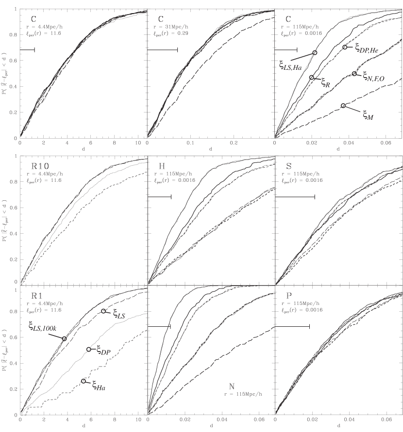
Fig. 1 shows the distribution
for the samples
described in Table 1. Three typical scales are
displayed to illustrate the general behavior. The principal
conclusions to be drawn are the following:
Small scales (): the effect of any boundary correction scheme becomes negligible, and as expected, all the estimators exhibit nearly identical behavior. The same is true for the samples S, P, N, and H not shown. However, some of the estimators are more sensitive to the density of random points, especially the Hamilton estimator, followed by the Davis–Peebles estimator. They show stronger deviations for the R1 and R10 samples due to the poor sampling of the term (see also Pons–Bordería et al. 1999). This effect persists on large scales as well.
Intermediate scales (): similar to the small scales. The Minus estimator shows stronger deviation becoming even more pronounced for the S, P, and H samples, since the effective remaining volume decreases.
Large scales (): edge corrections are becoming important, and the estimators exhibit clear differences in their distributions of the deviations for the samples C, and N. For a given probability, the Minus estimator shows the largest deviations, followed by the Natural, Fiksel and Ohser estimators. Significantly smaller deviations are obtained for the Davis–Peebles and Hewett estimators, and yet smaller for the Rivolo estimator. Finally, the Hamilton and LS estimator display the smallest deviations and thus the best edge correction. The two latter distributions nearly overlap. The above conclusions are robust and only weakly influenced by the presence of cutout holes, as seen from the H sample. The geometry of the subsamples has a non–trivial effect on the distributions. While the deviations are increased in the S and P samples, the differences between the estimators are reduced in the S, becoming negligible in the P samples. In both cases, the Minus estimator is not usable any more, since the equal zero, whereas the Fiksel estimator is biased for such geometries on large scales (this is implicitly shown in the work of Ohser (1983)).
Following Szapudi and Szalay (1999) the variance of the LS estimator may be calculated for a Poisson process:
| (6) |
with . The calculated for the considered samples is also shown in Fig. 1 to illustrate how much discreteness effects contribute to the distribution of the deviations. For our choice of sample parameters, the discreteness contribution, i.e. the deviation of a corresponding Poisson sample, is always within a factor of few of other important contributions to the variance, such as finite volume and edge effects. In general, the ratio of discreteness effects to the full variance depends in a complicated non–linear fashion on the number of clusters in the sample, the shape of the survey, integrals over the two–point correlation function and its square, and the three– and four–point correlation functions (see Szapudi et al. 2000 for the exact calculation). Varying the side length of the cubic samples from , , to we explored the influence of the size of the sample on the discreteness effects. Still, the rank order of the estimators stayed invariant.
4 Summary and Conclusion
For a sample with 222,052 clusters extracted from the Virgo Hubble volume simulation a reference two–point correlation function was determined. Within over 500 subsamples several estimators for the two–point correlation function were employed, and the results compared with the reference value. On small scales all the estimators are comparable. On large scales the LS and the Hamilton estimator significantly outperform the rest, showing the smallest deviations for a given cumulative probability. While the two estimators yield almost identical results for infinite number of random points, the Hamilton estimator is considerably more sensitive to the number of random points employed than the LS version. From a practical point of view the LS estimator is thus preferable. The rest of the estimators can be divided into three categories: The first runner–ups are the estimators from Rivolo, Davis–Peebles and Hewett, but already with a significantly increased variance. Even larger deviations are present for the Natural, Fiksel, and Ohser recipes. The Minus estimator has the largest deviation. Although it was shown that for special point processes both the LS and Hamilton estimator are biased (Kerscher, 1999), the present numerical experiment demonstrates that this is irrelevant for the realistic galaxy and cluster point processes, as the bias has an insignificant effect on the distribution of deviations. Pons–Bordería et al. (1999) did not recommend one estimator for all cases. In contrast, through our extensive numerical treatment the LS estimator emerges as a clear recommendation.
The above considerations apply to volume limited samples. When the correlation function is estimated directly from a flux limited sample with an appropriate minimum variance pair weighting (Feldman et al. (1994)), the Hamilton estimator has the advantage of being independent of the the normalization of the selection function.
The differences between the estimators become smaller for the slice and insignificant for the pencil beam samples. At first sight this is counter intuitive: the difference between the estimators is largely due to edge corrections, and less compact surveys obviously have more edges. For the large scale considered, S and P become essentially two– and one–dimensional and the weight is equal for most of the pairs separated by . Since the geometric estimators are approximately unbiased they employ mainly the same weight on large scales, and consequently show the same distribution of deviations. This argument also applies to the pair estimators, since they may be written in terms of these weights (Kerscher, 1999).
All the above numerical investigations are intimately related to the problem of calculating the expected errors on estimators for correlation functions. To include all contributions, such as edge, discreteness, and finite volume effects, the method by Colombi et al. (1994), Szapudi and Colombi (1996), Colombi et al. (1998), Szapudi et al. (1999) has to be extended for the two point correlation function. Such a calculation was performed by Szapudi et al. (2000), (see also Stoyan et al. 1993, Bernstein 1994 and Hamilton 1993 for approximations) and should be used for ab initio error calculations.
It is worth to mention, that one of the most widely used method in the literature, “bootstrap”, is based on a misunderstanding of the concept. For bootstrap in spatial statistics, a whole sample takes the role of one point in the original bootstrap procedure. This means that replicas of the original surveys would be needed to fulfill the promise of the bootstrap method. Choosing points (i.e. individual galaxies, clusters, etc.) randomly from one sample, as usually done, yields a variance with no obvious relation to the variance sought (see also Snethlage 1999).
The role of the random samples is to represent the shape of the survey in a Monte–Carlo fashion. A practical alternative is to put a fine grid on the survey and calculate the quantities , and , where now represents bin–counts and the indicator function taking the value one for pixels inside the survey, and zero otherwise. According to SS, all the above estimators have an analogous “grid” version (see also Hamilton 1993) which can be obtained formally by the substitution . In practice grid estimators can be more efficient than pair counts, and except for a slight perturbation of the pair separation bins, they both yield almost identical results for scales larger than a few pixel size.
The usual way of estimating the power spectrum, using a folding with the Fourier transform of the sample geometry is equivalent to the grid version of the LS estimator. Hence, such a power spectrum analysis extracts the same amount of information from the data as the analysis with the two–point correlation function using the grid version of the LS estimator. The results are only displayed with respect to a different basis. Similarly, Karhunen–Loève (KL) modes form another set of basis functions (Vogeley and Szalay, 1996). The uncorrelated power spectrum (Hamilton, 2000) and the KL modes are the methods of choice for cosmological parameter estimation. The KL modes allow for a well–defined cut–off, and therefore reduce the computational needs in a maximum likelihood analysis. However, geometrical features of the galaxy and cluster distribution directly show up in two–point correlation function and may be interpreted easily. Each bin of the two–point correlation function contains direct information on pairs separated by a certain distance, an intuitively simple concept more suitable to study and control (expected or unexpected) systematics (geometry, luminosity, galaxy properties, biases) than any other representation. In this sense the correlation function is a tool complementary to the power spectrum.
Acknowledgments
We are grateful to the Virgo Supercomputing Consortium
http://star-www.dur.ac.uk/$^∼$frazerp/virgo/virgo.html, who
made the Hubble volume simulation data available for our project. The
simulation was performed on the T3E at the Computing Centre of the
Max-Planck Society in Garching. We would like to thank Simon White
and the referee Andrew Hamilton for useful suggestions and
discussions. MK would like to thank Claus Beisbart and Dietrich Stoyan
for interesting and helpful discussions. IS was supported by the
PPARC rolling grant for Extragalactic Astronomy and Cosmology at
Durham while there. MK acknowledges support from the Sonderforschungsbereich für Astroteilchenphysik SFB 375 der DFG.
AS has been supported by NSF AST9802980 and NASA LTSA NAG653503.
References
- Bernstein (1994) G. M. Bernstein. 1994, ApJ, 424, 569.
- Colberg et al. (1998) J. M. Colberg, S. M. D. White, T. J. MacFarland, A. Jenkins, C. S. Frenk, F. R. Pearce, A. E. Evrard, H. M. P. Couchman, G. Efstathiou, J. A. Peacock, and P. A. Thomas. 1998, in Wide Field Surveys in Cosmology, 14th IAP meeting in Paris, eds. S. Colombi and Y. Mellier (Château de Blois: Editions Frontières), 247.
- Colombi et al. (1994) S. Colombi, F. Bouchet, and R. Schaeffer. 1994, A&A, 281, 301.
- Colombi et al. (1998) S. Colombi, I. Szapudi, and A. S. Szalay. 1998, MNRAS, 296, 253.
- Davis and Peebles (1983) M. Davis and P. J. E. Peebles. 1983, ApJ, 267, 465.
- Feldman et al. (1994) H. A. Feldman, N. Kaiser, and J. A. Peacock. 1994, ApJ, 426, 23.
- Fiksel (1988) T. Fiksel. 1988, Statistics, 19, 67.
- Hamilton (2000) A. J. S. Hamilton. 2000, MNRAS, 312, 257.
- Hamilton (1993) A. J. S. Hamilton. 1993, ApJ, 417, 19.
- Hewett (1982) P. C. Hewett. 1982, MNRAS, 201, 867.
- Heinrich (1988) L. Heinrich. 1988, Statistics, 19, 87.
- Kerscher (1999) M. Kerscher. 1999, A&A, 343, 333.
- Landy and Szalay (1993) S. D. Landy and A. S. Szalay. 1993, ApJ, 412, 64.
- Ohser (1983) J. Ohser. 1983, Math. Operationsforsch. u. Statist., Ser. Statist., 14, 63.
- Ohser and Stoyan (1981) J. Ohser and D. Stoyan. 1981, Biom. J., 23, 523.
- Pons–Bordería et al. (1999) M.-J. Pons–Bordería, V. J. Martínez, D. Stoyan, H. Stoyan, and E. Saar. 1999, ApJ, 523, 480.
- Ripley (1976) B. D. Ripley. 1976, J. Appl. Prob., 13, 255.
- Ripley (1988) B. D. Ripley. 1988, Statistical Inference For Spatial Processes (Cambridge: Cambridge University Press)
- Rivolo (1986) A. R. Rivolo. 1986, ApJ, 301, 70.
- Snethlage (1999) M. Snethlage. 1999, Metrika, 49, 245 (math.PR/0002061).
- Stoyan et al. (1993) D. Stoyan, U. Bertram and H. Wendrock. 1993, Ann. Inst. Satist. Math., 45, 211.
- Stoyan et al. (1995) D. Stoyan, W. S. Kendall, and J. Mecke. 1995, Stochastic Geometry and its Applications (Chichester: Wiley)
- Stoyan and Stoyan (2000) D. Stoyan and H. Stoyan. 2000, Scand. J. Satist., in press.
- Sylos Labini et al. (1998) F. Sylos Labini, M. Montuori, and L. Pietronero. 1998, Phys. Rep., 293, 61.
- Szapudi and Colombi (1996) I. Szapudi and S. Colombi. 1996, ApJ, 470, 131.
- Szapudi et al. (1999) I. Szapudi, S. Colombi, and F. Bernardeau. 1999, MNRAS, accepted.
- Szapudi et al. (2000) I. Szapudi, S. Colombi, and A. S. Szalay. 2000, in preparation.
- Szapudi and Szalay (1998) I. Szapudi and A. S. Szalay. 1998, ApJ, 494, L41.
- Szapudi and Szalay (1999) I. Szapudi and A. S. Szalay. 1999, Annales de l’I.S.U.P, in press.
- Vogeley and Szalay (1996) M. S. Vogeley and A. S. Szalay. 1996, ApJ, 465, 34.
| C | S | P | H | N | R1/R10 | |
| [Mpc/h] | 375 | 1000 | 130 | 375 | 375 | 375 |
|---|---|---|---|---|---|---|
| [Mpc/h] | 375 | 52.6 | 3000 | 375 | 375 | 375 |
| 512 | 513 | 529 | 512 | 512 | 512 | |
| 434 | 433 | 420 | 434 | 434 | 434 | |
| 100k | 100k | 100k | 100k | 100k | 1k/10k |