3D General Relativistic Simulations of Coalescing
Binary Neutron Stars

Abstract

We develop a 3 dimensional computer code to study a coalescing neutron star binary. The code can currently follow the evolution up to two stars begin to merge from two spherical stars of mass $1M_{\odot}$ and radius 8.9km with separation 35.4km. As for coordinate conditions, we use conformal slicing and pseudo-minimal distortion conditions. The evolution equations for the metric is integrated using the CIP method while the van Leer’s scheme is used to integrate the equations for the matter. We present a few results of our simulations including gravitational radiation.

1 Introduction

We report on the present status of our computer code development to study the fully general relativistic evolution of spacetimes and matter. We solve the complete set of the Einstein equations in the absence of any symmetries. The main motivation of this project is studying promising sources of strong gravitational waves, such as coalescing neutron star or black hole binaries. The first detection by an interferometric detector of gravitational waves such as LIGO, VIRGO, GEO600 and TAMA may be the waves from a black hole binary (see the contributions of K.S. Thorne, S. Kawamura and B. Schutz in this volume), but the astrophysical importance of a coalescing neutron star binary is not smaller than a black hole binary. A detailed analysis of the detected waves near the merger of two stars, for example, will give information on the size of a neutron star and then on the equation of state of high density matter. On problems other than the gravitational wave physics, study on process of coalescence of a neutron star binary is helpful for models of a source of a gamma ray burst (see the contribution of P.I. Meszaros in this volume).

A compact star binary in the earliest stage is almost stationary but gravitational radiation reaction makes it evolve in the adiabatic manner. When the separation between stars is large enough, the stars can be regarded as point particles. As the separation is getting small, however, the size effect of the stars and the relativistic effects become important. Thus the complete set of the Einstein equations and the general relativistic hydrodynamics equations for a neutron star binary must be solved. In addition, the process of coalescence of a binary is not axisymmetric. Thus a three dimensional (in space) code is necessary and it requires a great power of computers. In 1994, we became able to use a supercomputer with memories of tens of GBytes and a peak speed of nearly a hundred GFLOPS. With this computer, we can manage a $200^{3}$ grid. Then we started to make a 3D, fully general relativistic code for a coalescing neutron star binary. In this paper, we show the present status of our code development. The present code does not include a lot of realistic physics processes such as neutrino emission and a realistic equation of state near and beyond the nuclear density. So it is a milestone of 3D numerical relativity. In §2, we describe the mathematical framework of the calculation, including constraint equations, evolution equations of the metric, relativistic hydrodynamics equations, coordinate conditions and evaluation of the gravitational waves. In §3, numerical methods we use for elliptic equations and evolution equations are shown. In §4, we present numerical results of simulations of coalescing neutron star binaries obtained using the present code. In §5, we summarize and outline future work planned for this code.

2 The Mathematical Framework

2.1 Constraint equations

In the (3+1) (or ADM) formalism of general relativity, the spacetime metric is written as

$$ds^{2}=-\alpha^{2}dt^{2}+\gamma_{ij}(dx^{i}+\beta^{i}dt)(dx^{j}+\beta^{j}dt),$$ (1)

where $\alpha$, $\beta^{i}$ and $\gamma_{ij}$ are the lapse function, the shift vector and the intrinsic metric of three-metric. The Einstein equation reduces to the four constraint equations

$$R+K^{2}-K_{ij}K^{ij}=16\pi\rho_{{}_{H}},$$ (2)

$$D_{j}\left(K^{j}{}_{i}-\delta^{j}{}_{i}K\right)=8\pi J_{i}$$ (3)

and 12 evolution equations

$$\partial_{t}\gamma_{ij}=-2\alpha K_{ij}+D_{i}\beta_{j}+D_{j}\beta_{i},$$ (4)

$$\partial_{t}K_{ij} = \alpha\left[R_{ij}-8\pi\left\{S_{ij}+\mbox{$\frac{1}{2}$}\gamma_{ij}\left(\rho_{{}_{H}}-S^{\ell}{}_{\ell}\right)\right\}\right]-D_{i}D_{j}\alpha$$ (5)

$$+\alpha\left(KK_{ij}-2K_{i\ell}K^{\ell}{}_{j}\right)+K_{\ell i}D_{j}\beta^{\ell}+K_{\ell j}D_{i}\beta^{\ell}+\beta^{\ell}D_{\ell}K_{ij},$$

where $R_{ij}$ is the Ricci tensor, $K_{ij}$ the extrinsic curvature tensor, $K=K^{\ell}{}_{\ell}$, and $D_{i}$ the covariant derivative associated with $\gamma_{ij}$. The quantities $\rho_{{}_{H}}$, $J_{i}$ and $S_{ij}$ are the energy density, the momentum density and the stress tensor, respectively, measured by the observer moving along the line normal to the spacelike hypersurface of $t=$constant.

In order to give an initial data, we should find a three-metric and extrinsic curvature which satisfy the constraint equations (2) and (3). It means that the constraint equations are solved giving $\rho_{{}_{H}}$ and $J_{i}$. Here we assume that $K=0$ and $\gamma_{ij}$ is conformally flat at $t=0$

$$\gamma_{ij}=\phi^{4}\,\widetilde{\gamma}_{ij},$$ (6)

where $\widetilde{\gamma}_{ij}$ is the flat space metric. Defining the conformal transformation as

$$\begin{array}[c]{l}\widetilde{K}_{ij}\equiv\phi^{2}K_{ij},\qquad\widetilde{K}_{i}{}^{j}\equiv\phi^{6}K_{i}{}^{j},\qquad\widetilde{K}^{ij}\equiv\phi^{10}K^{ij},\\ \rho_{{}_{B}}\equiv\phi^{6}\rho_{{}_{H}}\qquad\mbox{and}\qquad\widetilde{J}_{i}\equiv\phi^{6}J_{i},\end{array}$$ (7)

Eq.(3) reduces to

$$\widetilde{D}_{j}\widetilde{K}^{j}{}_{i}=8\pi\widetilde{J}_{i},$$ (8)

where $\widetilde{D}_{i}$ is the covariant derivative associated with $\widetilde{\gamma}_{ij}$.[1] The traceless extrinsic curvature can be decomposed with the transverse traceless part $\widetilde{K}^{\mbox{\scriptsize TT}}_{ij}$ and the longitudinal traceless part $(LW)_{ij}$ [2];

$$\widetilde{K}_{ij}=\widetilde{K}^{\mbox{\scriptsize TT}}_{ij}+(LW)_{ij},$$ (9)

where

$$(LW)_{ij}=\widetilde{D}_{i}W_{j}+\widetilde{D}_{j}W_{i}-\frac{2}{3}\,\widetilde{\gamma}_{ij}\widetilde{D}^{\ell}W_{\ell}.$$ (10)

Assuming $\widetilde{K}^{\mbox{\scriptsize TT}}_{ij}=0$, Eq.(8) becomes

$$\widetilde{\triangle}W_{i}+\frac{1}{3}\widetilde{D}_{i}\widetilde{D}^{j}W_{j}=8\pi\widetilde{J}_{i},$$ (11)

where $\widetilde{\triangle}\equiv\widetilde{D}^{i}\widetilde{D}_{i}$. Equation (11) is the coupled elliptic equation but can be reduced to four decoupled Poisson equations:

$$\triangle\chi=6\pi\partial_{i}\widetilde{J}_{i},$$ (12)

$$\triangle W_{i}=8\pi\widetilde{J}_{i}-\frac{1}{3}\partial_{i}\chi,$$ (13)

where $\chi=\partial_{i}W_{i}$.

The Hamiltonian constraint equation (2) reduces to the nonlinear Poisson equation

$$\widetilde{\triangle}\phi=-2\pi\phi^{-1}\rho_{{}_{B}}-\frac{1}{8}\phi^{-7}\widetilde{K}_{ij}\widetilde{K}^{ij}.$$ (14)

2.2 Evolution equations of the metric

Defining the following variables

$$\phi=\left(\mbox{det}(\gamma_{ij})\right)^{\frac{1}{12}},\qquad\widetilde{\gamma}_{ij}=\phi^{-4}\gamma_{ij}\ ,\qquad\widetilde{\gamma}^{ik}\widetilde{\gamma}_{kj}=\delta^{i}{}_{j},$$ (15)

$$\widehat{K}_{ij}=\mbox{STF}(\phi^{-4}K_{ij}),\qquad\widehat{K}^{i}{}_{j}=\widetilde{\gamma}^{ik}\widehat{K}_{kj}\ ,\qquad\widehat{K}^{ij}=\widetilde{\gamma}^{jk}\widehat{K}^{i}{}_{k},$$ (16)

where

$$\mbox{STF}(A_{ij})\equiv\frac{1}{2}\left(A_{ij}+A_{ji}-\frac{2}{3}\widetilde{\gamma}_{ij}\widetilde{\gamma}^{k\ell}A_{k\ell}\right),$$ (17)

the evolution equation (5) reduces to

$$\partial_{t}\widehat{K}_{ij}-\beta^{\ell}\partial_{\ell}\widehat{K}_{ij} = \phi^{-4}\left[\mbox{STF}\left\{\alpha\left(R_{ij}-8\pi S_{ij}\right)-D_{i}D_{j}\alpha\right\}\right]$$

$$+ \alpha\left(K\widehat{K}_{ij}-2\widehat{K}_{i\ell}\widehat{K}^{\ell}{}_{j}\right)$$

$$+ \widehat{K}_{i\ell}\partial_{j}\beta^{\ell}+\widehat{K}_{j\ell}\partial_{i}\beta^{\ell}-\frac{2}{3}\widehat{K}_{ij}\partial_{\ell}\beta^{\ell},$$

$$\partial_{t}K-\beta^{\ell}\partial_{\ell}K = \alpha\!\left[\widehat{K}_{ij}\widehat{K}^{ij}\!+\!\frac{1}{3}K^{2}\!+\!4\pi\!\left(\rho_{{}_{H}}\!+\!S^{i}{}_{i}\right)\right]\!-\!D^{i}D_{i}\alpha,$$ (19)

and Eq.(4) to

$$\partial_{t}\widetilde{\gamma}_{ij}=-2\left[\alpha\widehat{K}_{ij}-\mbox{STF}\left\{\widetilde{D}_{i}\left(\phi^{-4}\beta_{j}\right)\right\}\right]\equiv A_{ij}$$ (20)

or

$$\partial_{t}\widetilde{\gamma}_{ij}-\beta^{\ell}\partial_{\ell}\widetilde{\gamma}_{ij}=-2\!\left[\alpha\widehat{K}_{ij}-\mbox{STF}\left(\widetilde{\gamma}_{i\ell}\partial_{j}\beta^{\ell}\right)\right].$$ (21)

The conformal factor $\phi$ obeys

$$\partial_{t}\phi-\beta^{\ell}\partial_{\ell}\phi=-\frac{\phi}{6}\left(\alpha K-\partial_{\ell}\beta^{\ell}\right)$$ (22)

or

$$\widetilde{\triangle}\phi=-\frac{\phi^{5}}{8}\left(16\pi\rho_{{}_{H}}+K_{ij}K^{ij}-K^{2}-\phi^{-4}\widetilde{R}\right).$$ (23)

Equation (22) follows from the trace of Eq.(4), while Eq.(23) from the Hamiltonian constraint (2).

2.3 Relativistic hydrodynamics equations

We assume the perfect fluid stress-energy tensor, which is given by

$$T_{\mu\nu}=(\rho+\rho\varepsilon+p)u_{\mu}u_{\nu}+pg_{\mu\nu},$$ (24)

where $\rho$, $\varepsilon$ and $p$ are the proper mass density, the specific internal energy and the pressure, respectively, and $u_{\mu}$ is the four-velocity of the fluid. The energy density $\rho_{{}_{H}}$, the momentum density $J_{i}$ and the stress tensor $S_{ij}$ of the matter measured by the normal line observer are, respectively, given by

$$\rho_{{}_{H}}\equiv n^{\mu}n^{\nu}T_{\mu\nu},\ \ J_{i}\equiv-h_{i}{}^{\mu}n^{\nu}T_{\mu\nu}\ \ \mbox{and}\ \ S_{ij}\equiv h_{i}{}^{\mu}h_{j}{}^{\nu}T_{\mu\nu},$$ (25)

where $n_{\mu}$ is the unit timelike four-vector normal to the spacelike hypersurface and $h_{\mu\nu}$ is the projection tensor into the hypersurface defined by

$$h_{\mu\nu}=g_{\mu\nu}+n_{\mu}n_{\nu}.$$ (26)

The relativistic hydrodynamics equations are obtained from the conservation of baryon number, $\nabla_{\mu}(\rho u^{\mu})$, and the energy-momentum conservation law, $\nabla_{\nu}T_{\mu}{}^{\nu}{}$. In order to obtain equations similar to the Newtonian hydrodynamics equations, we define $\rho_{{}_{N}}$ and $u_{i}^{N}$ as

$$\rho_{{}_{N}}\equiv\sqrt{\gamma}\alpha u^{0}\rho\ \ \ \mbox{and}\ \ \ u_{i}^{N}=\frac{J_{i}}{\alpha u^{0}\rho},$$ (27)

respectively, where $\gamma=\mbox{det}(\gamma_{ij})$. Then the equation for the conservation of baryon number takes the form

$$\partial_{t}\rho_{{}_{N}}+\partial_{\ell}\left(\rho_{{}_{N}}V^{\ell}\right)=0,$$ (28)

where

$$V^{\ell}=\frac{u^{\ell}}{u^{0}}=\frac{\alpha J^{\ell}}{p+\rho_{{}_{H}}}-\beta^{\ell}.$$ (29)

The equation for momentum conservation is

$$\partial_{t}(\rho_{{}_{N}}u_{i}^{N})+\partial_{\ell}\left(\rho_{{}_{N}}u_{i}^{N}V^{\ell}\right) = -\sqrt{\gamma}\alpha\partial_{i}p-\sqrt{\gamma}(p+\rho_{{}_{H}})\partial_{i}\alpha$$ (30)

$$\frac{\sqrt{\gamma}\alpha J^{k}J^{\ell}}{2(p+\rho_{{}_{H}})}\partial_{i}\gamma_{k\ell}+\sqrt{\gamma}J_{\ell}\partial_{i}\beta^{\ell}.$$

The equation for internal energy conservation becomes

$$\partial_{t}(\rho_{{}_{N}}\varepsilon)+\partial_{\ell}\left(\rho_{{}_{N}}\varepsilon V^{\ell}\right)=-p\partial_{\nu}\left(\sqrt{\gamma}\alpha u^{\nu}\right).$$ (31)

To complete hydrodynamics equations, we need an equation of state,

$$p=p(\varepsilon,\rho).$$ (32)

The right-hand side of Eq.(31) includes the time derivative. For a polytropic equation of state, $p=(\Gamma-1)\rho\varepsilon$, however, the equation reduces to

$$\partial_{t}(\rho_{{}_{N}}\varepsilon_{{}_{N}})+\partial_{\ell}\left(\rho_{{}_{N}}\varepsilon_{{}_{N}}V^{\ell}\right)=-p_{{}_{N}}\partial_{\ell}V^{\ell},$$ (33)

where

$$\varepsilon_{{}_{N}} = \left(\sqrt{\gamma}\alpha u^{0}\right)^{\Gamma-1}\,\varepsilon,$$ (34)

$$p_{{}_{N}} = (\Gamma-1)\rho_{{}_{N}}\varepsilon_{{}_{N}}=\left(\sqrt{\gamma}\alpha u^{0}\right)^{\Gamma}p.$$ (35)

2.4 Coordinate conditions and gravitational waves

The choice of a shift vector $\beta^{i}$ and a lapse function $\alpha$ is important because the stability of the code largely depends on it and because it is intimately related to the extraction of physically relevant information, including gravitational radiation, in numerical relativity.

Since the right-hand side of Eq.(20), $A_{ij}$ is trace-free, the determinant of $\widetilde{\gamma}_{ij}$ is preserved in time and the condition

$$D^{j}A_{ij}=0$$ (36)

produces the minimal distortion shift vector.[3] It must be a good choice of the spatial coordinate, but it is too complicated to be solved. Instead we replace the covariant derivative by the partial derivative

$$\partial_{i}A_{ij}=0,$$ (37)

which yields an elliptic equation for the shift vector $\beta^{i}$:

$$\nabla^{2}\beta^{i}+\frac{1}{3}\partial_{i}\partial_{\ell}\beta^{\ell}=2\partial_{j}\left[\alpha\widehat{K}_{ij}-\mbox{STF}(h_{i\ell}\partial_{j}\beta^{\ell})-\frac{1}{2}\beta^{\ell}\partial_{\ell}h_{ij}\right],$$ (38)

where

$$h_{ij}=\widetilde{\gamma}_{ij}-\delta_{ij}.$$ (39)

We call this condition as the pseudo-minimal distortion condition.

As for slicing condition, we choose the conformal slicing,[4] where the lapse function $\alpha$ is given by

$$\alpha=\exp\left[-2\left(\widehat{\phi}+\frac{\widehat{\phi}^{3}}{3}+\frac{\widehat{\phi}^{5}}{5}\right)\right]$$ (40)

with $\widehat{\phi}=\phi-1$. Since in this slicing,

$$\alpha\approx\frac{1-\widehat{\phi}}{1+\widehat{\phi}}\rightarrow\frac{1-\frac{M}{2r}}{1+\frac{M}{2r}}$$ (41)

for large $r$, the space outside the central matter quickly approaches the Schwarzschild metric in the isotropic coordinates. Thus $h_{ij}$ defined by Eq.(39) can be considered as gravitational wave parts for large $r$ and the total energy of the gravitational waves is given by

$$E_{\mbox{\scriptsize GW}}=\int dt\int_{r\rightarrow\infty}d\Omega\ r^{2}\,\rho_{{}_{\mbox{\scriptsize GW}}},$$ (42)

$$\rho_{{}_{\mbox{\scriptsize GW}}}=\frac{1}{32\pi}A_{ij}A_{ij},$$ (43)

since Eq.(37) means that $A_{ij}$ is the transverse-traceless part of the time derivative of $\widetilde{\gamma}_{ij}$ for large $r$.

3 Numerical Methods

3.1 Coordinate system

As for the spatial coordinates, we use a Cartesian coordinate system $(x,y,z)$. We solve partial differential equations (PDEs) using a finite-difference scheme, where a finite grid is introduced and the PDEs are replaced by finite-difference approximations. It may be convenient to use a spherical coordinate system $(r,\theta,\phi)$ with regard to saving of computer memory and an outer boundary condition at large distance from a compact source. But the use of spherical coordinates leads to a vexing problem of coordinate singularities at the origin and along the polar axis.

3.2 Elliptic equations

The constraint equations reduce four Poisson equations (12) and (13), and a nonlinear Poisson equation (14). These equations are solved once for initial data. The shift vector is given by the coupled elliptic equation (38), which is solved at every time step. The conformal factor $\phi$ is, in turn, determined either by the hyperbolic equation (22) or by the elliptic equation (Hamiltonian constraint) (23). However, since it is known that the conformal slicing yields instability in $\phi$ and $\alpha$,[5] we solve the Hamiltonian constraint (23) at every time step to prevent the onset of the instability caused by numerical errors from occurring quickly. Thus the solution of the elliptic equations consumes the greatest part of the CPU time.

A non-linear equation such as

$$\triangle\phi(t)=-4\pi S(\phi(t)),$$ (44)

where $S(\phi)$ is a non-linear function of $\phi$, must be solved by an iterative method:

$$\phi^{(I+1)}=\triangle^{-1}S\left(\phi^{(I)}\right)\quad\mbox{for $I=0,1,2,\cdots$}.$$ (45)

To solve Eq.(14) for initial data, we should made the iteration. For Eq.(23), however, we don’t made the iteration to reduce the required CPU time. Instead, the right-hand side $S(\phi(t))$ is calculated using an approximate value of $\phi(t)$ evaluated by extrapolation from the values of $\phi$ at the previous two time steps $t-\Delta t$ and $t-2\Delta t$. We examined the difference of the solution using the extrapolated source from the solution obtained by the iterative method, and found that it is small enough if $\Delta t$ is as small as we use for our actual calculations.

We use the extrapolated value of $\beta^{i}$ in calculating the right-hand side of Eq.(38), too. Note that terms including $\beta^{i}$ vanish and we don’t need the extrapolated value at $t=0$, since $h_{ij}=0$. Thus Eq.(38) reduces four Poisson equations (12) and (13), replacing $W_{i}$ to $\beta^{i}$.

Now all the elliptic equations reduce Poisson equations, which are solved using a pre-conditioned conjugate gradient method.[6] The boundary condition of $\phi$ giving by Eq.(44) is that

$$\phi=\frac{M}{r}+\frac{d_{x}x^{k}}{r^{3}}+O\left(\frac{1}{r^{3}}\right),$$ (46)

for large $r$, where

$$M=\int S\,d^{3}x,\qquad d_{k}=\int Sx^{k}\,d^{3}x.$$ (47)

The boundary condition of $\chi$ and $W_{i}$ (or $\beta^{i}$) giving by Eqs.(12) and (13) is that[6]

$$\chi = \frac{P_{i}x^{i}}{2r^{3}}-\frac{3M_{ii}}{2r^{3}}+\frac{9M_{ij}x^{i}x^{j}}{2r^{5}}+O\left(\frac{1}{r^{4}}\right),$$ (48)

$$W_{i} = -\frac{P_{k}x^{k}x^{i}}{4r^{3}}-\frac{7P_{i}}{4r}$$ (49)

$$-\frac{\left(7M_{ij}-M_{ji}-M_{kk}\delta_{ij}\right)x^{j}}{4r^{3}}-\frac{3M_{jk}x^{j}x^{k}x^{i}}{4r^{5}}+O\left(\frac{1}{r^{3}}\right)$$

for large $r$, where

$$P_{i}=\int\widetilde{J}_{i}\,d^{3}x,\qquad M_{ij}=\int\widetilde{J}_{i}x^{j}\,d^{3}x.$$ (50)

3.3 Evolution of matter

Hydrodynamics equations Eqs.(28), (30) and (33) are written as

$$\partial_{t}Q+\partial_{\ell}(QV^{\ell})=F,$$ (51)

which is split into two phases:

$$\partial_{t}Q+\partial_{\ell}(QV^{\ell})=0,$$ (52)

$$\partial_{t}Q=F.$$ (53)

Here we call Eq.(52) the advection phase and Eq.(53) the non-advection phase. The advection phase is solved using van Leer’s scheme[7] to obtain $Q^{(n+1)*}_{ijk}$ from $Q^{n}_{abc}$ and $(V^{\ell})^{n}_{abc}$, where $Q^{n}_{abc}$ is the value of $Q$ at $n$-th time step $t=t^{n}$ and a spatial grid point $(x^{a},y^{b},z^{c})$. If the non-advection phase is solved as

$$Q^{n+1}_{ijk}=Q^{(n+1)*}_{ijk}+\Delta t\cdot F^{n}_{ijk}$$ (54)

with $F^{n}_{ijk}$ calculated using quantities at $t=t^{n}$, it is of first-order accuracy in time. To achieve second-order accuracy, we use (1) a two-step algorithm

$$Q^{n+\frac{1}{2}}_{ijk} = Q^{(n+\frac{1}{2})*}_{ijk}+\frac{1}{2}\Delta t\cdot F^{n}_{ijk},$$ (55)

$$Q^{n+1}_{ijk} = Q^{(n+1)*}_{ijk}+\Delta t\cdot F^{n+\frac{1}{2}}_{ijk},$$ (56)

where $Q^{n+\frac{1}{2}}_{ijk}$ is used only in calculating $F^{n+\frac{1}{2}}_{ijk}$, or (2) a extrapolated source algorithm

$$Q^{n+1}_{ijk}=Q^{(n+1)*}_{ijk}+\Delta t\cdot\widetilde{F}^{n+\frac{1}{2}}_{ijk},$$ (57)

where $\widetilde{F}^{n+\frac{1}{2}}_{ijk}$ given by

$$\widetilde{F}^{n+\frac{1}{2}}_{ijk}=F^{n}_{ijk}+\frac{1}{2}(F^{n}_{ijk}-F^{n-1}_{ijk})$$ (58)

is the value of $F$ at $t=t^{n}+\frac{1}{2}\Delta t$ evaluated by extrapolation from the values at $t=t^{n}$ and $t=t^{n}-\Delta t$. Since some test calculations indicated that these algorithms give almost the same results if $\Delta t$ is small, we will use the extrapolated source algorithm.

Since the outer boundary is sufficiently far from the region of the matter distribution, we can safely set $Q=0$ at the outer boundary.

3.4 Evolution of metric

The evolution equations for $\widehat{K}_{ij}$ (2.2), $K$ (19) and $\widetilde{\gamma}_{ij}$ (21) can be written as

$$\partial_{t}Q+v^{\ell}\partial_{\ell}Q=F,$$ (59)

with $v^{\ell}=-\beta^{\ell}$. It is solved using the CIP (Cubic-Interpolated Pseudoparticle/Propagation) method.[8] In the CIP method, both Eq.(59) and its spatial derivatives

$$\partial_{t}(\partial_{a}Q)+v^{\ell}\partial_{\ell}(\partial_{a}Q)=-(\partial_{i}v^{\ell})(\partial_{\ell}Q)+\partial_{a}F$$ (60)

are solved. Numerical diffusion during propagation of $Q$ can be reduced, since the time evolution of $Q$ and its derivatives are traced. Equations (59) and (60) are split into the advection and the non-advection phases similarly to Eqs.(52) and (53). In the non-advection phase, $F$ and $\partial_{a}F$ at $t=t^{n}+\frac{1}{2}\Delta t$ are evaluated by extrapolation from the values at previous two time steps.

By the way, special care must be taken to calculate the Ricci tensor appearing in the right-hand side of Eq.(2.2). With conformal transformation Eq.(15), the Ricci tensor $R_{ij}$ associated with $\gamma_{ij}$ is given by

$$R_{ij}=\widetilde{R}_{ij}+R^{(\phi)}_{ij},$$ (61)

where

$$R^{(\phi)}_{ij} = -2\phi^{-1}\left(\widetilde{D}_{j}\widetilde{D}_{i}\phi+\widetilde{\gamma}_{ij}\widetilde{\triangle}\phi\right)$$ (62)

$$+2\phi^{-2}\left(3(\widetilde{D}_{i}\phi)(\widetilde{D}_{j}\phi)-\widetilde{\gamma}_{ij}(\widetilde{D}_{k}\phi)(\widetilde{D}^{k}\phi)\right)$$

and $\widetilde{R}_{ij}$ is the Ricci tensor associated with $\widetilde{\gamma}_{ij}$, which is given by

$$\widetilde{R}_{ij}=\frac{1}{2}\left[\widetilde{\gamma}^{k\ell}\left(h_{\ell i,jk}+h_{\ell j,ik}-h_{ij,k\ell}\right)+\widetilde{\gamma}^{k\ell}{}_{,k}\left(h_{\ell i,j}+h_{\ell j,i}-h_{ij,\ell}\right)\right]-\widetilde{\Gamma}^{k}_{\ell i}\widetilde{\Gamma}^{\ell}_{jk}.$$ (63)

The second derivatives of $h_{ij}$ are replaced by finite differences in numerical calculation but the numerical precision of terms such as $h_{ij,k\ell}$ with $k\neq\ell$ is not so good, while the degree of precision in calculation of $h_{ij,k\ell}$ with $k=\ell$ is the same as that of the first derivatives. Inaccuracies in $h_{ij,k\ell}$ will cause a numerical instability. The ‘pseudo-minimal distortion condition’, Eq.(37), however, leads $\delta^{jk}h_{ij,k}=0$ and therefore

$$\widetilde{\gamma}^{k\ell}\left(h_{\ell i,jk}+h_{\ell j,ik}-h_{ij,k\ell}\right)=-h_{ij,kk}+\psi^{k\ell}\left(h_{\ell i,jk}+h_{\ell j,ik}-h_{ij,k\ell}\right),$$ (64)

where $\psi^{ij}=\widetilde{\gamma}^{ij}-\delta^{ij}$. Inaccuracies in numerical values of $\psi^{k\ell}h_{\ell i,jk}$ will not affect integration of Eq.(2.2) so seriously since both $\psi^{k\ell}$ and $h_{\ell i,jk}$ are smaller than unity.

Boundary conditions for $\widehat{K}_{ij}$ and $\widetilde{\gamma}_{ij}$ are important, because the boundary is not so far from the stars and therefore inappropriate boundary conditions cause reflections of the outgoing waves. We apply outgoing conditions for $\widetilde{K}_{ij}$ and $\widetilde{\gamma}_{ij}$, since non-wave parts decrease rapidly in our coordinate conditions. The condition can be written as

$$Q(t,x^{i})=\frac{H(\alpha t-\phi^{2}r)}{r},$$ (65)

where $r=\sqrt{x^{2}+y^{2}+z^{2}}$. Here $H$ satisfies an advection equation

$$\partial_{t}H+c^{\ell}\partial_{\ell}H=0,$$ (66)

where

$$c^{\ell}=\frac{\alpha x^{\ell}}{r\phi^{2}}.$$ (67)

It implies

$$\partial_{t}Q+c^{\ell}\partial_{\ell}Q=-\frac{\alpha}{r\phi^{2}}.$$ (68)

Equation (68) is solved along with Eq.(59) using the CIP method.

4 Numerical Simulations of Coalescing Binary Neutron Stars

Now we show numerical results on simulations of coalescing binary neutron stars. As for a equation of state, we use the $\gamma=2$ polytropic equation of state. To reduce the required memory, we assume the symmetry with respect to the equatorial ($z=0$) plane. A uniform grid of size $191\times 191\times 96$ with $\Delta x=\Delta y=\Delta z=1GM_{\odot}/c^{2}=1.5$km is used. The numerical boundary is located at $95GM_{\odot}/c^{2}$ from the origin. In order to keep precision, we set the time step $\Delta t$ as 0.01$GM_{\odot}/c^{3}=5\times 10^{-8}$ seconds. Calculations are performed on Fujitsu VPP500/80 at High Energy Accelerator Research Organization (KEK) and Fujitsu VPP300/16R at the National Astronomical Observatory (NAO), Japan. The required memory is approximately 8GBytes.

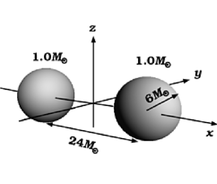
Figure 1: Initial configuration of a coalescing neutron star binary.

4.1 Initial data

We performed calculations with two kinds of initial data. One is the corotation (synchronized rotation) case as for ordinary stellar binaries, in which the momentum density $\widetilde{J}_{i}$ appearing in Eq.(8) of each star is given by

$$\widetilde{J}_{i}=\rho_{{}_{B}}\epsilon_{ijk}\Omega^{j}x^{k},$$ (69)

where $\epsilon_{ijk}$ is the complete antisymmetric symbol and the angular velocity $\Omega^{j}$ is constant. The other is the irrotational (zero-circulation) case as for gravitational radiation driven compact stellar binaries, in which $\widetilde{J}_{i}$ is given by

$$\widetilde{J}_{i}=\rho_{{}_{B}}\epsilon_{ijk}\Omega^{j}x^{k}_{c},$$ (70)

where $x^{k}_{c}$ is the position of each star and is constant for an individual star. In both cases, we assume that the binary consists of identical spherical stars of rest mass $1.0M_{\odot}$, radius 8.9km located at $(x_{c},y_{c},z_{c})=(\pm 17.7\mbox{km},0,0)$. The orbital angular momentum $\Omega$ points to the $z$-direction.

Table 1: Parameters of initial data. The angular momentum parameter $q$ is $J_{t}/(GM_{\mbox{\scriptsize tot}}^{2}/c)$.

	Corotation	Irrotation
Orbital angular velocity $\Omega$ [sec-1]	$2.4\times 10^{3}$	$2.4\times 10^{3}$
Angular momentum $J_{t}$ [$GM_{\odot}^{2}/c$]	3.9	3.5
Collision velocity $v_{x}$ [$c$]	0.074	0.071
Total gravitational mass $M_{\mbox{\scriptsize tot}}$ [$M_{\odot}$]	1.96	1.95
Angular momentum parameter $q$	1.03	0.93

4.2 Corotation case

The parameters of initial data for the corotation case are shown in the second column of Table 1. It take about 10 hours on VPP500 using 64 processor units up to 26000 time steps. Figure 2 shows the evolution of the density and the velocity on the $x$-$y$ plane. Movies for it including the evolution on $x$-$z$ and $y$-$z$ planes can be obtained from our Web site.[9] At the $\sim$26000th time step, the onset of instability on $\phi$ in the central region occurs and it grows exponentially in a few time steps. At the time, only 3 grid points or so are included from the center to the surface of the star. So that numerical errors grow on account of unstable modes resident in the conformal slicing.

A thick disk around the merged star is likely to be formed as shown in Fig. 3. The mass of the disk is about a few percent of the total mass. In addition, there are indications of outflow along the rotation axis. However, since the precision of the numerical calculation at this time is not so good, these facts must be confirmed with more precise calculation.

The propagation of the “energy density of gravitational waves” $r^{2}\rho_{{}_{\mbox{\scriptsize GW}}}$ is shown in Fig. 4, movies of which are also provided on our Web site.[9] A spiral pattern appears on the $x$-$y$ plane, while different patterns with peaks around $z$-axis appear on the $x$-$z$ plane. This can be explained naively by the quadrupole wave pattern given by

$$r^{2}\rho_{{}_{\mbox{\scriptsize GW}}}=\frac{r^{2}}{32\pi}\left(A_{ij}\right)^{2}\propto\cos^{2}\theta+\sin^{2}\theta\sin^{2}(2\Omega(t-r)-2\varphi)/4.$$ (71)

On the $x$-$y$ plane, where $\theta=\pi/2$, $\rho_{{}_{\mbox{\scriptsize GW}}}$ is constant along the spiral of $r+\varphi/\Omega=$ constant, while near $z$-axis, where $\theta\approx 0$, $\rho_{{}_{\mbox{\scriptsize GW}}}\propto\cos^{2}\theta$.

Figure 2: Density $\rho_{{}_{N}}$ and velocity $V^{i}$ on the $x$-$y$ plane for the corotation case. Time in units of milliseconds is shown. Solid lines are drawn from $\rho_{\mbox{\scriptsize min}}$ through $\rho_{\mbox{\scriptsize max}}$ in steps of $\rho_{\mbox{\scriptsize min}}$, where $\rho_{\mbox{\scriptsize min}}=8\times 10^{14}$g$\cdot$cm^-3 and $\rho_{\mbox{\scriptsize max}}=4\times 10^{16}$g$\cdot$cm^-3. Dashed lines are at 1/2, 1/4, 1/8, 1/16, 1/32 of $\rho_{\mbox{\scriptsize min}}$.

Figure 3: Density $\rho_{{}_{N}}$ and velocity $V^{i}$ in the central region on the $x$-$y$, $x$-$z$ and $z$-$y$ planes for the corotation case. Parameters for contour lines are the same as Fig. 2 but $\rho_{\mbox{\scriptsize max}}=3.41\times 10^{16}$g$\cdot$cm^-3 and $\rho_{\mbox{\scriptsize min}}=0.1\rho_{\mbox{\scriptsize max}}$.

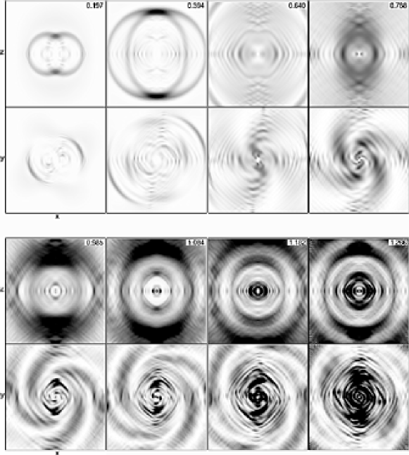
Figure 4: The propagation of the gravitational waves for the corotation case. The “energy densities of gravitational waves” $r^{2}\rho_{{}_{\mbox{\scriptsize GW}}}$ on the $x$-$y$ and $x$-$z$ planes are shown as gray scale figures up to the numerical boundary. Time in units of milliseconds is shown. The upper figure of each time is on $x$-$z$ plane and the lower one is on $x$-$y$ plane.

Figure 5: Waveforms $h_{+}$ and $h_{\times}$ observed on the $z$-axis for the corotation case. They have been monitored at $r=75M_{\odot},80M_{\odot}$ and $85M_{\odot}$.

Figure 6: Luminosity (in units of erg/sec) and total energy (in units of erg) of the emitted gravitational waves. They are evaluated at $r=75M_{\odot},80M_{\odot}$ and $85M_{\odot}$.

The waves pass through the numerical boundary with little reflection. It means that the boundary condition Eq.(68) behaves well. However, a small reflection on the $x$-, $y$- and $z$-axes interfere with the outgoing waves and interference patterns appears after $t\sim 0.8$msec.

Figures 6 shows the waveforms on the $z$-axis monitored between $75M_{\odot}$ and $85M_{\odot}$ from the origin. The emitted waveform falls off with $r^{-1}$ as expected. The luminosity evaluated between $75M_{\odot}$ and $85M_{\odot}$ as functions of $t$ and the total energy of the gravitational waves up to $t$ are shown in Fig. 6. Comparing Figs. 4, 6 and 6 with Fig. 2, the main part of the waves begins to be emitted when the merger develops to a certain extend, but only the waves up to the time when the merger begins have arrived at the numerical boundary. The minor peak around $t-r=0$ corresponds the waves included unexpectedly in the initial data.

The amplitude of gravitational waves is

$$h=5\times 10^{-22}\left(\frac{r}{10\mbox{Mpc}}\right)$$ (72)

and the total energy emitted is

$$E_{\mbox{\scriptsize GW}}(t<1\mbox{msec})=10^{-3}M_{\odot}c^{2}=2\times 10^{51}\mbox{erg}\sim 0.05\%\mbox{ of }M_{\mbox{\scriptsize tot}}c^{2}.$$ (73)

The angular momentum of the emitted gravitational waves is given by

$$\Delta J=\int\frac{dJ}{dt}\,dt,$$ (74)

$$\frac{dJ}{dt}=\frac{1}{16\pi}\int\epsilon_{zjk}x^{j}(h^{\mbox{\scriptsize TT}}_{km,p}\dot{h}^{\mbox{\scriptsize TT}}_{mp}-\frac{1}{2}h^{\mbox{\scriptsize TT}}_{mp,k}\dot{h}^{\mbox{\scriptsize TT}}_{mp})\,dS,$$ (75)

to be

$$\Delta J(t<1\mbox{msec})=1.8\times 10^{-2}GM_{\odot}^{2}/c\sim 0.5\mbox{\% of }J_{t}.$$ (76)

4.3 Irrotation case

The parameters of initial data for the irrotation case are shown in the third column of Table 1. The evolution of the density and the velocity on the $x$-$y$ plane are shown in Fig. 7.[9]

The propagation of the “energy density of gravitational waves” $r^{2}\rho_{{}_{\mbox{\scriptsize GW}}}$ are shown in Fig. 9,[9] the waveforms on the $z$-axis in Fig. 11 and the energy of the waves in Fig. 11.

Figure 7: Density $\rho_{{}_{N}}$ and velocity $V^{i}$ on the $x$-$y$ plane for the irrotation case. Parameters are the same as Fig 2.

Figure 8: Density $\rho_{{}_{N}}$ and velocity $V^{i}$ in the central region on the $x$-$y$, $x$-$z$ and $z$-$y$ planes for the irrotation case. Parameters are the same as Fig. 3.

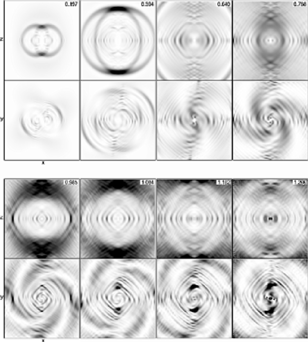
Figure 9: The propagation of the gravitational waves for the irrotation case. The “energy densities of gravitational waves” $r^{2}\rho_{{}_{\mbox{\scriptsize GW}}}$ on the $x$-$y$ and $x$-$z$ planes are shown similarly to Fig. 4

Figure 10: Waveforms $h_{+}$ and $h_{\times}$ observed on the $z$-axis for the irrotation case. They have been monitored at $r=75M_{\odot},80M_{\odot}$ and $85M_{\odot}$.

Figure 11: Luminosity (in units of erg/sec) and total energy (in units of erg) of the emitted gravitational waves. They are evaluated at $r=75M_{\odot},80M_{\odot}$ and $85M_{\odot}$.

The evolution is in principle the same as the corotation case, but no outflow along the rotation axis appears in Fig. 8. It is because the merger is progressing slower. It is the case in post-Newtonian calculations also that the progress of the merger for the irrotation case is slower than for the corotation case.[6] It causes the emission of gravitational waves to decrease somewhat. The amplitude, the energy and the angular momentum of the gravitational waves emitted up to 1msec are, however, almost the same as in the corotation case:

$$h=5\times 10^{-22}\left(\frac{r}{10\mbox{Mpc}}\right),$$

$$E_{\mbox{\scriptsize GW}}(t<1\mbox{msec})\sim 0.05\%\mbox{ of }M_{\mbox{\scriptsize tot}}c^{2},$$ (77)

$$\Delta J(t<1\mbox{msec})\sim 0.5\mbox{\% of }J_{t}.$$

5 Summary

We have described a numerical code for simulations of coalescing binary neutron stars and presented some results with it. This code was developed after extensive study of a post-Newtonian code for coalescing binary neutron stars.[6] To solve hydrodynamics equations and elliptic equations, the general relativistic code uses the same methods as the post-Newtonian code does. For evolution equations for the metric, however, we adopted the CIP method, which made the evolution of the metric stable even with a coarse grid.

We faced instability when coalescence of two stars advanced to be probably a black hole. It is caused by a characteristics of the conformal slicing as well as by the coarseness of the grid. This fact may suggest that other slicing such as the maximal slicing must be adopted. Thus we are now making another code with the maximal slicing. With the maximal slicing, we must solve a elliptic equation for $\alpha$, which is obtained by setteing the right-hand side of Eq.(19) equal to zero. The cost of solving this equation is great. In addition, to catch the wave form of gravitational waves, we have to apply a gauge-invariant wave extraction technique.[10] Since new super computer, 7 times faster with 20 times greater memory, will be available at KEK from the beginning of 2000, more precise calculation with the maximal slicing will be carried out. To calculate the right-hand side of Eq.(38), we used the extrapolated values for $\beta^{i}$ as describe in §3.2, but the precision of the extrapolation will reduce in the highly dynamical phase of coalescence. We will be able to solve Eq.(38) more precisely by an iterative method on the new machine.

References

- [1] J.W. York Jr., Source of Gravitational Radiation (Cambridge University Press, Cambridge, 1979), p.83.
- [2] J.W. York Jr., \JLJ. Math. Phys.,14,1973,456.
- [3] L. Smarr and J.W. York Jr., \PRD17,1978,1945.
- [4] M. Shibata and T. Nakamura, \PTP88,1992,317.
- [5] M. Shibata and T. Nakamura, \PRD52, 1995, 5428.
- [6] K. Oohara, T. Nakamura and M. Shibata, Prog. Theor. Phys. Suppl. No. 128 (1997), 183.
- [7] B. van Leer, \JLJ. Comput. Phys.,23,1977,276.
- [8] T. Yabe, in Computational Fluid Dynamics Review 1997 (Wiley, 1997).
-
[9]
http://astro.sc.niigata-u.ac.jp/~oohara/ykis99/. - [10] A. Abrahams, D. Bernstein, D. Hobill, E. Seidel and L. Smarr, \PRD50,1992,3544.