Physical State of Molecular Gas in High Galactic Latitude Translucent Clouds

Abstract

The rotational transitions of carbon monoxide (CO) are the primary means of investigating the density and velocity structure of the molecular interstellar medium. Here we study the lowest four rotational transitions of CO towards high–latitude translucent molecular clouds (HLCs). We report new observations of the J = (4–3), (2–1), and (1–0) transitions of CO towards eight high–latitude clouds. The new observations are combined with data from the literature to show that the emission from all observed CO transitions is linearly correlated. This implies that the excitation conditions which lead to emission in these transitions are uniform throughout the clouds. Observed ${}^{13}{\rm C}$O/${}^{12}{\rm C}$O  (1–0) integrated intensity ratios are generally much greater than the expected abundance ratio of the two species, indicating that the regions which emit ${}^{12}{\rm C}$O (1–0) radiation are optically thick. We develop a statistical method to compare the observed line ratios with models of CO excitation and radiative transfer. This enables us to determine the most likely portion of the physical parameter space which is compatible with the observations. The model enables us to rule out CO gas temperatures greater than $\sim 30{\,{\rm K}}$, since the most likely high-temperature configurations are 1$\,{\rm pc}\mkern-5.0mu$ -sized structures aligned along the line of sight. The most probable solution is a high density and low temperature (HDLT) solution, with volume density, $n={10^{4.5\pm 0.5}}{\,{\rm cm}^{-3}}$, kinetic temperature, ${{\rm T_{\rm k}}}\approx 8{\,{\rm K}}$, and CO column density per velocity interval ${{{\rm N}_{\rm\scriptscriptstyle CO}/{\Delta{\rm V}}}}={10^{16.6\pm 0.3}}{\,{\rm cm}^{-2}}/({\,{\,{\rm km}}{\,{\rm s}}^{-1}})$. The CO cell size is $L\sim 0.01{\,{\rm pc}}$ ($\sim 2000\,$AU). These cells are thus tiny fragments within the $\sim$100 times larger CO-emitting extent of a typical high–latitude cloud. We discuss the physical implications of HDLT cells, and we suggest ways to test for their existence.

1. Introduction

The rotational transitions of carbon monoxide (CO) are the most important probes used to trace the density and velocity structure of molecular clouds. Due to the low electric dipole moment of the CO molecule, the J = (1–0) and (2–1) transitions are easily excited into emission in molecular clouds with modest extinctions (${{\rm A}_{\rm v}}\gtrsim 1\,$ magnitude). Because of this and the fact that the frequencies of the (1–0) and (2–1) transitions lie in two relatively transparent atmospheric windows, they are the most commonly observed molecular emission lines in the interstellar medium (ISM). Unfortunately the information given by observing these transitions is limited, since they are not sensitive to volume densities above the critical density for collisional excitation, ${{\rm n}_{\rm\scriptscriptstyle crit}}\sim 10^{3}{\,{\rm cm}^{-3}}$. To probe gas at higher density demands that transitions with higher energies be observed. Star-formation regions are bright in the high-J CO transitions, but modelling these transitions is difficult because (1) the large CO column density in such regions renders their interiors completely opaque, and (2) randomly distributed energy sources (stars) increase dramatically the complexity of the problem. Modelling success is more likely in regions which are relatively optically thin and far from star formation.

The simplest class of molecular cloud observable in CO is the translucent cloud (van Dishoeck & Black 1988). Translucent clouds have modest visual extinctions (${{\rm A}_{\rm v}}\approx 1-5\,$mag), and therefore are intermediate between low-extinction diffuse clouds, which contain few molecules observable in emission, and optically thick dark clouds. The high Galactic latitude ($b\gtrsim 15\arcdeg$) molecular clouds (HLCs; see review by Magnani, Hartmann, & Speck 1996, and references therein) are a set of nearby ($\langle d\rangle\approx 105{\,{\rm pc}}$; Magnani et al. 1996) translucent clouds associated with IRAS cirrus (Low et al. 1984). The HLCs are generally far from sources of far-ultraviolet (FUV) (6 eV $<h\nu<$ 13.6 eV) radiation and most are probably exposed to the average interstellar FUV radiation field (see van Dishoeck & Black 1988; Draine 1978; Habing 1968). High–latitude clouds are photochemically and energetically the simplest molecular objects in the ISM. They have equal amounts of carbon gas in atomic form, C I, as in CO, with an average C/CO column density ratio of $\sim 1$ (Stark & van Dishoeck 1994; Ingalls, Bania, & Jackson 1994; Ingalls, et al. 1997). They are essentially isolated photodissociation regions (Tielens & Hollenbach 1985) whose structure is dominated by the transition from atomic to molecular gas which occurs on the surface of all molecular clouds. Most HLCs are uncomplicated by internal energy sources. Some of the HLCs contain T Tauri stars (Magnani, Caillault, Buchalter, & Beichman 1995; Pound 1996) and others have marginally bound dense cores (Reach et al. 1995), but on the whole HLCs are minimally affected by stars. Thus they are the most basic clouds observable in CO emission and are ideal candidates for multi-transition CO studies.

The most comprehensive study of CO in translucent and high–latitude clouds was done by van Dishoeck, Black, Phillips, & Gredel (1991). They observed 4 transitions of ${}^{12}{\rm C}$O and ${}^{13}{\rm C}$O in a sample of $\sim 25$ clouds. They derived relatively low gas volume densities ($n=200-5000{\,{\rm cm}^{-3}}$) and high kinetic temperatures (${{\rm T_{\rm k}}}>20{\,{\rm K}}$), but they warned that their data are also compatible with higher densities and lower temperatures. An ongoing investigation of the physics and chemistry of translucent clouds (Turner 1994; see also Turner, Terzieva, & Herbst 1999 and references therein) supports the low density, high temperature conclusion. On the other hand, a study of CO emission towards the translucent edge of a cloud in the Perseus–Auriga complex (Falgarone & Phillips 1996, hereafter FP) claimed that the CO emission is produced by beam–diluted clumps with high densities ($n>{10^{4}}{\,{\rm cm}^{-3}}$) and low temperatures (${\rm T_{\rm\scriptscriptstyle k}}\lesssim 15{\,{\rm K}}$) (see also Falgarone, Phillips, & Walker 1991). Interestingly, FP admitted that the observations could also be produced by a more homogeneous CO medium with lower densities ($n\sim 200{\,{\rm cm}^{-3}}$) and higher temperatures (${{\rm T_{\rm k}}}\sim 30-50{\,{\rm K}}$).

In general the solution of the statistical equilibrium equations rests on an assumption about either the kinetic temperature or the cloud geometry (van Dishoeck et al. 1991). Clearly such solutions are not unique, since collisional excitation rates are affected by both temperature and density. Observations of the rotational transitions of high dipole-moment molecules in translucent and high–latitude clouds (Reach, Pound, Wilner & Lee 1995; Heithausen, Corneilussen, & Grossman 1998) support the assertion made by FP that significant quantities of dense gas exist, but they do not prove that most of the CO emission originates in such gas. Even the high-density conclusions of Reach et al. (1995), and Heithausen et al. (1998) rely on assumed low ${\rm T_{\rm k}}$ values (5–20$\,{\rm K}\mkern-5.0mu$ ).

The CO emission towards translucent clouds shows some surprising regularities which should be exploited in a multitransition study. For example, the ${}^{12}{\rm C}$O (2–1) intensity is linearly proportional to the (1–0) intensity in clouds without star formation, for all positions and velocities observed (FP; Falgarone et al. 1998). This important fact implies that the excitation conditions which lead to emission in these transitions are uniform throughout the clouds. FP argued that the simplest situation which would produce uniform excitation conditions was the high density, low temperature (HDLT) one ($n>{10^{4}}{\,{\rm cm}^{-3}};{{\rm T_{\rm k}}}\sim 10{\,{\rm K}}$), since the CO level populations would be thermal under these conditions. They eliminated the low density, high temperature (LDHT) case ($n<{10^{4}}{\,{\rm cm}^{-3}};{{\rm T_{\rm k}}}\gtrsim 20{\,{\rm K}}$) because the implied line-of-sight structure sizes (column density divided by volume density) are greater than the $\sim 0.06$$\,{\rm pc}\mkern-5.0mu$  size of the smallest structure observed in projection on the plane of the sky. Implicit in their argument is the assumption that the size of a structure along the line-of-sight equals (on average) the size of the smallest observed structure in the plane of the sky.

This may not be strictly true. The best direct evidence for the existence of tiny CO clumps in translucent clouds is the population of unresolved $\sim 2000$ AU (0.01$\,{\rm pc}\mkern-5.0mu$  )–sized structures seen in velocity channel maps of the first IRAM key-project (Falgarone et al. 1998). These dense unresolved cores are not isolated spheres, however, but usually have the shape of elongated filaments which are unresolved in one direction only. Thus there is little reason to suppose that the average line of sight size of CO emission cells equals the smallest observed plane-of-sky structure size.

Given this geometrical uncertainty, data for many transitions are needed to decide if the primary source of CO emission is gas with LDHT or HDLT conditions. In particular, higher energy transitions of CO should be observed towards translucent clouds. Although they observed the (4–3) transition of ${}^{12}{\rm C}$O towards some positions in the cloud they studied, FP were not able to determine if excitation of this transition was uniform, as it was for the (1–0) and (2–1) transitions. If the CO level populations are thermal, then the discovery of uniform J = 4 excitation might support their claim of the ubiquity of gas with $n>{10^{4}}{\,{\rm cm}^{-3}}$, since the critical density for thermal excitation of the (4–3) transition is $\sim{10^{4-5}}{\,{\rm cm}^{-3}}$.

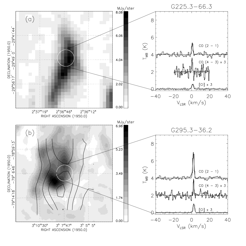
Figure 1.— Observations of high–latitude clouds. The greyscale maps show HIRES-processed IRAS 100µm emission. Black contours represent AST/RO ${}^{12}{\rm C}$O (J = 2–1) integrated intensity. A 5′ circle is drawn on each map in white, at the nominal source position, defined by Keto & Myers (1986). The average ${}^{12}{\rm C}$O (2–1), ${}^{12}{\rm C}$O (4–3), and [C I] (${}^{3}{\rm P}_{\rm\scriptscriptstyle 1}\rightarrow{{}^{3}\rm P}_{\rm\scriptscriptstyle 0}$) spectra measured in this circle with AST/RO are shown on the right. Gaussian fits are superimposed on the spectra. The C I data were originally published by Ingalls et al. (1997). The ${}^{12}{\rm C}$O (4–3) and C I intensities have been multiplied by 3. (a) Cloud G225.3–66.3. This source was not mapped in ${}^{12}{\rm C}$O (2–1) emission. (b) Cloud G295.3–36.2. Contours of ${}^{12}{\rm C}$O (2–1) emission range from 2.2 to 2.8 K$\,{\,{\rm km}}{\,{\rm s}}^{-1}\mkern-5.0mu$ , in 2.2 K$\,{\,{\rm km}}{\,{\rm s}}^{-1}\mkern-5.0mu$  intervals.

In this paper we report observations of the J = (4–3) rotational transition of ${}^{12}{\rm C}$O towards a sample of 8 translucent high–latitude molecular clouds at southern declinations (§2 and §3). Our new data are used in conjunction with the ${}^{12}{\rm C}$O and ${}^{13}{\rm C}$O observations made by van Dishoeck et al. (1991) to constrain the physical conditions in the HLC regions emitting CO radiation (§4). We show that the emission from all CO transitions up to (4–3) is linearly correlated, i.e., the excitation is uniform. We use a statistical argument to demonstrate that inclusion of our new (4–3) data narrows significantly the allowed region of parameter space, making the HDLT solution the most likely one. We discuss the physical implications of gas with HDLT properties, particularly thermal pressure imbalance with the ambient interstellar medium (§5). Finally we suggest a method to test for the existence of HDLT gas.

2. Observations

2.1. The source sample

Eight HLCs at southern declinations were observed (see Table 1 for Galactic identifications). Seven of the clouds were listed in the catalog of Keto & Myers (1986). The observed source positions are listed in Ingalls et al. (1997). In addition, a previously unknown translucent high–latitude cloud, G259.4–13.3 [$\alpha(1950.0)=7^{h}29^{m}42^{s};~{}\delta(1950.0)=-47\arcdeg 00\arcmin 41\arcsec$], was observed. This cloud was discovered during a search made towards IRAS cirrus clouds for new ${}^{12}{\rm C}$O (2–1) sources (Ingalls 1999).

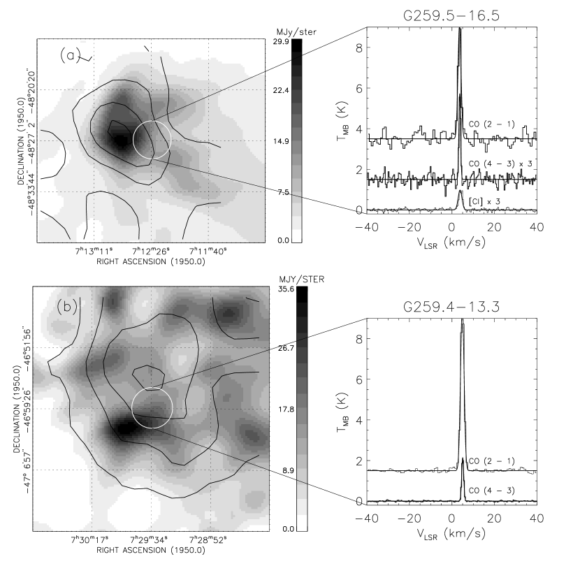
Figure 2.— Observations of high–latitude clouds. See caption to Figure 1 for description. (a) Cloud G259.5–16.5. Contours of ${}^{12}{\rm C}$O (J = 2–1) emission range from 1.9 to 7.6 K$\,{\,{\rm km}}{\,{\rm s}}^{-1}\mkern-5.0mu$ , in 1.9 K$\,{\,{\rm km}}{\,{\rm s}}^{-1}\mkern-5.0mu$  intervals. (b) Cloud G259.4–13.3, discovered by Ingalls (1999), with nominal source position taken from that work. Contours of ${}^{12}{\rm C}$O (2–1) emission range from 7.7 to 30.8 K$\,{\,{\rm km}}{\,{\rm s}}^{-1}\mkern-5.0mu$ , in 7.7 K$\,{\,{\rm km}}{\,{\rm s}}^{-1}\mkern-5.0mu$  intervals.

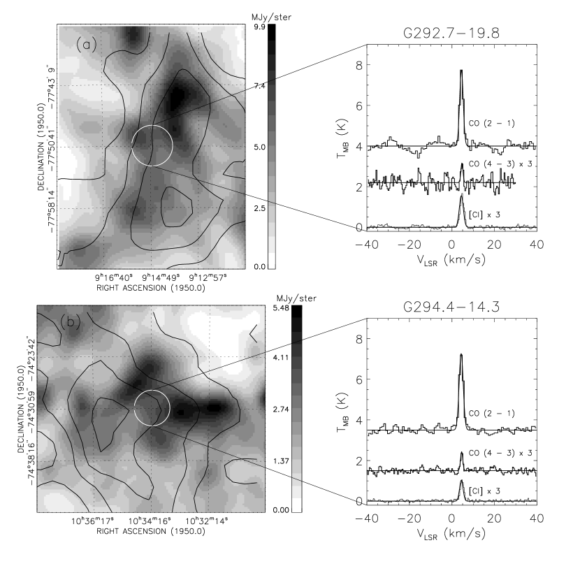
Figure 3.— Observations of high–latitude clouds. See caption to Figure 1 for description. (a) Cloud G292.7–19.8. Contours of ${}^{12}{\rm C}$O (J = 2–1) emission range from 2.8 to 9.9 K$\,{\,{\rm km}}{\,{\rm s}}^{-1}\mkern-5.0mu$ , in 2.4 K$\,{\,{\rm km}}{\,{\rm s}}^{-1}\mkern-5.0mu$  intervals. (b) Cloud G294.4–14.3. Contours of ${}^{12}{\rm C}$O (2–1) emission range from 2.4 to 9.9 K$\,{\,{\rm km}}{\,{\rm s}}^{-1}\mkern-5.0mu$ , in 2.5 K$\,{\,{\rm km}}{\,{\rm s}}^{-1}\mkern-5.0mu$  intervals.

The observations described here were part of a study of the overall gas-phase carbon content in translucent clouds (Ingalls, Bania, & Jackson 1994; Ingalls et al. 1997; Ingalls 1999). The seven clouds from the Keto & Myers (1986) catalog were each recently detected in neutral atomic carbon [C I] emission by Ingalls et al. (1997). Prior to this, most of the clouds had only been observed in CO at 8$\farcm$7 angular resolution (Keto & Myers 1986). Cloud G225.3–66.3, has also been observed at higher resolution in CO emission and in the photographic B band by Stark (1995).

Cloud G316.5+21.0 has a low mass star embedded in it (Ingalls et al. 1997). Since this cloud has its own internal energy source it may be hotter and more dense than the typical HLC. A comparison with the more quiescent clouds in the sample may provide insight into the effects of low mass star formation on translucent gas.

2.2. AST/RO Observations of CO (4–3) and (2–1) emission

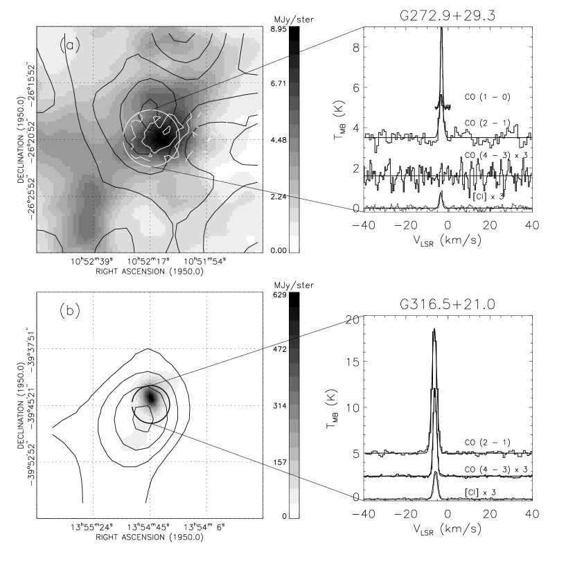
Figure 4.— Observations of high–latitude clouds. The data shown here correspond to those described in the caption to Figure 1, with the addition of FCRAO ${}^{12}{\rm C}$O (1–0) data in part a. (a) Cloud G272.9+29.3. White contours of ${}^{12}{\rm C}$O (J = 1–0) emission range from 1.9 to 3.9 K$\,{\,{\rm km}}{\,{\rm s}}^{-1}\mkern-5.0mu$ in 1.9 K$\,{\,{\rm km}}{\,{\rm s}}^{-1}\mkern-5.0mu$  intervals. The average (1–0) spectrum is superimposed on the plot at right. Black contours of ${}^{12}{\rm C}$O (J = 2–1) emission range from 0.6 to 3.0 K$\,{\,{\rm km}}{\,{\rm s}}^{-1}\mkern-5.0mu$ in 0.6 K$\,{\,{\rm km}}{\,{\rm s}}^{-1}\mkern-5.0mu$  intervals. The ${}^{12}{\rm C}$O (4–3) line was not detected from this source and the nondetection spectrum is shown. (b) Cloud G316.5+21.0. Contours of ${}^{12}{\rm C}$O (2–1) emission range from 13.8 to 34.5 K$\,{\,{\rm km}}{\,{\rm s}}^{-1}\mkern-5.0mu$ , in 6.9 K$\,{\,{\rm km}}{\,{\rm s}}^{-1}\mkern-5.0mu$  intervals.

Observations of the 461.041 GHz (J = 4–3) transition of ${}^{12}{\rm C}$O were made during the period 1997 June 29 through July 13, using the Antarctic Submillimeter Telescope and Remote Observatory (AST/RO). AST/RO is a 1.7m diameter telescope located at the National Science Foundation Amundsen-Scott South Pole Station (Stark et al. 1997). The telescope efficiency at 461 GHz was estimated from skydip measurements (Chamberlin, Lane, & Stark 1997) to be $\eta_{l}=0.77$. As mentioned by Ingalls et al. (1997), $\eta_{l}$ is close to the main-beam efficiency, $\eta_{\rm\scriptscriptstyle MB}$. The 461 GHz transition was measured using the AST/RO 492/810 SIS waveguide receiver which had a $\sim 130{\,{\rm K}}$ double sideband receiver noise temperature. The intermediate frequency output was sampled by a 2048 channel, 1.4 GHz bandwidth acousto-optical spectrometer (AOS) (Schieder, Tolls, & Winnewisser 1989). The velocity resolution was $\delta$V${}_{\rm\scriptscriptstyle 461}=0.62{\,{\,{\rm km}}{\,{\rm s}}^{-1}}\,{\rm channel^{-1}}$. System noise temperatures were of order 1800–3000$\,{\rm K}\mkern-5.0mu$ . The half power beam width of the AST/RO telescope at 461 GHz was approximately 180″.

Observations of the 230.538 GHz (J = 2–1) transition of ${}^{12}{\rm C}$O were made in 1996 November using the AST/RO 230 GHz SIS receiver which had a double sideband noise temperature of $\sim 500{\,{\rm K}}$. Based on measurements of $\eta_{l}$ from skydips (see above), the value $\eta_{\rm\scriptscriptstyle MB}=0.54$ was adopted for 230 GHz. The same AOS used for the (4–3) measurements was used for the (2–1) data, yielding a velocity resolution of $\delta$V${}_{\rm\scriptscriptstyle 230}=1.34{\,{\,{\rm km}}{\,{\rm s}}^{-1}}\,{\rm channel^{-1}}$. The system noise temperature at 230 GHz was $\sim 1800{\,{\rm K}}$. The beamsize of the AST/RO telescope at 230 GHz is $\sim 5\arcmin$.

The ${}^{12}{\rm C}$O (4–3) and (2–1) observations were obtained by position-switching 1° in azimuth. Because of the location of AST/RO, position-switched offsets were both at constant elevation and at fixed positions on the sky. Intensity calibration was accomplished by measuring two blackbody loads at known temperatures (Stark et al. 1997). In order to correct for atmospheric attenuation the sky brightness temperature was measured at the position of a source every $\sim 15$ minutes. The overall intensity calibration was checked by observing periodically the compact H II region G291.2–0.8. This procedure yielded intensities repeatable to within $\pm 15\%$ at both 230 GHz and 461 GHz.

2.3. FCRAO observations of CO (1–0) towards cloud G272.9+29.3

The HLC G272.9+29.3 was observed with the Five College Radio Astronomy Observatory (FCRAO), in Amherst MA, on 1996 February 17 through 18. The FCRAO 14m telescope was used to map the ${}^{12}{\rm C}$O (1–0) transition at 115.2712 GHz. The telescope has a beamsize of 45″ and a 115 GHz main beam efficiency of $\eta_{\rm\scriptscriptstyle MB}\approx 0.36$ at 20° elevation (Ladd & Heyer 1996). The observations were carried out in frequency–switched mode, with the signal and reference spectra spaced 4.5 MHz apart. The spectra were measured with the QUARRY focal plane array receiver (Erickson et al. 1992), and the data were sampled by an array of 15 autocorrelation spectrometers with 1024 channels, separated by 77 kHz per channel, giving a velocity resolution of $\delta$V${}_{\rm\scriptscriptstyle 115}=0.2{\,{\,{\rm km}}{\,{\rm s}}^{-1}}\,{\rm channel^{-1}}$. Since the source is a Southern hemisphere object with declination $\delta=-26\arcdeg$, its elevation was rather low, ranging from 16° to 19°. The single–sideband system noise temperature was approximately 2000 K for these observations.

3. Observational Results

3.1. CO (4–3) and (2–1) Properties of HLCs

Observed ${}^{12}{\rm C}$O (4–3) and (2–1) spectra are plotted alongside maps of each source in Figures 1 to 4. The (4–3) transition was detected towards 7 of 8 clouds observed. The ${}^{12}{\rm C}$O (4–3) HLC data consist of half-beam sampled measurements made on a $\sim 5\arcmin\times 5\arcmin$ grid, in a manner similar to the C I “superbeam” observations described by Ingalls et al. (1997). These maps were averaged over the $5\arcmin$–square grids to produce the spectra shown in Figures 1 to 4. The C I “superbeam” average spectra taken towards the same positions (Ingalls et al. 1997) are also displayed in the figures. Intensities are main-beam brightness temperatures, ${\rm T}_{\rm\scriptscriptstyle MB}\mkern-5.0mu$ , i.e., Rayleigh-Jeans antenna temperature, $T_{A}$, corrected for both atmospheric attenuation and main-beam efficiency (${{\rm T}_{\rm\scriptscriptstyle MB}}\equiv T_{A}^{*}/\eta_{\rm\scriptscriptstyle MB}$).

Each source was observed in ${}^{12}{\rm C}$O (2–1) emission at its nominal center with the $\sim 5\arcmin$ AST/RO beam. For seven of the sources, these spectra are part of $\sim\,30\arcmin\times 30\arcmin$ half-beam sampled maps, shown as black contours overlaid on IRAS 100$\,\mu$m greyscale images in Figures 1 to 4. The IRAS images were all processed using the HIRES technique (Levine et al. 1993), and have angular resolution $\sim 100\arcsec$. The calibration uncertainty for the HIRES images is of order 20%.

Gaussian fits were made to the CO (4–3) and (2–1) spectra and are shown superimposed on these spectra in Figures 1 to 4. Table 1 lists the line center velocity, $\rm V_{\rm\scriptscriptstyle LSR}$, and the peak intensity, ${\rm T}_{\rm\scriptscriptstyle MB}\mkern-5.0mu$ , from the Gaussian fits. Also listed is the integrated line intensity, $\int{{\rm T}_{\rm\scriptscriptstyle MB}}dV$. Error bars for both transitions were determined by adding in quadrature the instrumental noise ($\Delta{\rm T_{\rm\scriptscriptstyle RMS}}$) and a calibration uncertainty of 15%:

$$\sigma({{\rm T}_{\rm\scriptscriptstyle MB}})=\sqrt{\left({{\Delta{\rm T_{\rm\scriptscriptstyle RMS}}}}\right)^{2}+\left(0.15{{\rm T}_{\rm\scriptscriptstyle MB}}\right)^{2}}.$$ (1)

Gaussian fit linewidths, $\Delta V$, range from 0.9 to 3$\,{\,{\rm km}}{\,{\rm s}}^{-1}\mkern-5.0mu$  with an average of $(1.7\pm 0.5)$$\,{\,{\rm km}}{\,{\rm s}}^{-1}\mkern-5.0mu$ , slightly greater than the velocity resolution of the (2–1) observations, so the lines are only marginally resolved. For this reason both ${\rm T}_{\rm\scriptscriptstyle MB}\mkern-5.0mu$  and $\Delta V$ are poorly-determined. We will therefore focus our attention on the integrated intensity, $\int{{\rm T}_{\rm\scriptscriptstyle MB}}dV$, which is a better defined quantity. Since (4–3) radiation was not detected towards G272.9+29.3, we estimate a 3$\sigma$ upper limit to the (4–3) integrated intensity for this source using the average linewidth: $\int{{\rm T}_{\rm\scriptscriptstyle MB}}(4-3)\,dV<3\times{{\Delta{\rm T_{\rm\scriptscriptstyle RMS}}}}\times 1.7{\,{\,{\rm km}}{\,{\rm s}}^{-1}}$.

3.2. The CO (1–0) Map of G272.9+29.3

The (1–0) transition of ${}^{12}{\rm C}$O was mapped in source G272.9+29.3 at 45″ angular resolution. The map consisted of a $29\times 11$ grid of pixels, evenly spaced at $\sim 25\arcsec$, one-half the FCRAO beamwidth. The resulting map of ${}^{12}{\rm C}$O (1–0) integrated intensity is superimposed as white contours on Figure 4 (a). The average spectrum in a $5\arcmin$ “superbeam” at the nominal source center is plotted on the right side of this figure. This spectrum was resolved in velocity by the FCRAO spectrometer: a Gaussian fit gives the line center velocity ${{\rm V_{\rm\scriptscriptstyle LSR}}}=-3.1$, linewidth $\Delta V=1.0$ and peak intensity ${{\rm T}_{\rm\scriptscriptstyle MB}}=5.6\pm 1.8$.

Figure 5.— The HLCs compared with typical Galactic emitters of infrared radiation. This plot shows the 60µm versus 100µm surface brightness of the sample clouds. A straight line denoting ${{\rm I}_{\rm\scriptscriptstyle 60}}=0.16{{\rm I}_{\rm\scriptscriptstyle 100}}$, the average behavior for Milky Way gas correlated with H I emission (Dwek et al. 1997), is superimposed. Note that this line is not a fit to the data.

3.3. The HLCs as Representative CO Clouds

The HLCs are the average Galactic high–latitude sources of CO emission. This can be shown in two ways. First, we can use the all-sky CO survey done with the Far Infrared Absolute Spectrometer (FIRAS) instrument on board the Cosmic Background Explorer (COBE) satellite. This instrument was used to observe nearly the entire sky at 7° resolution in the first six transitions of ${}^{12}{\rm C}$O (Wright et al. 1991; Bennett et al. 1994). The data are available on the World Wide Web. The average value of the COBE FIRAS high-latitude ($|b|>15\arcdeg$) (4–3)/(2–1) integrated intensity ratio is $\langle(4-3)/(2-1)\rangle_{\rm\scriptscriptstyle COBE}=0.84\pm 0.06$. The intensities were reported in units of erg$\,{\rm cm}^{-2}\mkern-5.0mu$ $\,{\rm s^{-1}}\mkern-5.0mu$  ${\rm sr}^{-1}$. The FIRAS integrated intensity ratio may be compared with the ratio of integrated Rayleigh-Jeans brightness temperatures measured here for HLCs if one uses the conversion formula:

$$\frac{\int I_{\nu}d\nu}{\rm erg{\,{\rm cm}^{-2}}{\,{\rm s^{-1}}}sr^{-1}}~{}=~{}Q(\nu)\,\frac{\int{{\rm T}_{\rm\scriptscriptstyle MB}}\,dV}{\rm K{\,{\,{\rm km}}{\,{\rm s}}^{-1}}}.$$ (2)

The function $Q(\nu)\equiv 2\times 10^{5}k\nu^{3}/c^{3}$: $Q(230)=1.25\times 10^{-8}$ and $Q(461)=10^{-7}$ erg$\,{\rm cm}^{-2}\mkern-5.0mu$ $\,{\rm s^{-1}}\mkern-5.0mu$  ${\rm sr}^{-1}/({\,{\rm K}}{\,{\,{\rm km}}{\,{\rm s}}^{-1}})$. The average HLC value measured here is [Equation 3, multiplied by $Q(461)/Q(230)=8$] $\langle(4-3)/(2-1)\rangle_{\rm\scriptscriptstyle HLC}=0.88\pm 0.16$, which is nearly identical to the COBE average.

Figure 6.— Observed ${}^{12}{\rm C}$O (J = 4–3) (Top) and (J = 2–1) (Bottom) properties of HLCs. The integrated main beam brightness temperature, $\int{{\rm T}_{\rm\scriptscriptstyle MB}}dV$, is plotted here for each transition as a function of IRAS 100µm surface brightness.

Figure 7.— Integrated main beam brightness temperature ${\rm I}_{\rm\scriptscriptstyle CO}\mkern-5.0mu$  (4–3) versus ${\rm I}_{\rm\scriptscriptstyle CO}\mkern-5.0mu$  (2–1). The straight line fit, $I_{(4-3)}=0.11I_{(2-1)}$, is superimposed.

The infrared properties of the HLCs studied here can also be compared with the average properties of interstellar cirrus clouds. HIRES-processed images of both 60 and 100µm emission observed with IRAS were obtained for each cloud in the sample. The 60µm surface brightness, ${\rm I}_{\rm\scriptscriptstyle 60}\mkern-5.0mu$ , is plotted as a function of the 100µm surface brightness, ${\rm I}_{\rm\scriptscriptstyle 100}\mkern-5.0mu$ , in Figure 5. Both the 60 and 100µm measurements are averages over the 5′ “superbeam” centered on each source, described in §3.1. The Diffuse Infrared Background Experiment (DIRBE) on board the COBE satellite was used to observe the infrared spectrum of the entire Galaxy. The average result for all Milky Way gas correlated with H I emission, $\langle{{\rm I}_{\rm\scriptscriptstyle 60}}/{{\rm I}_{\rm\scriptscriptstyle 100}}\rangle_{\rm\scriptscriptstyle COBE}=0.160$, was derived by Dwek et al. (1997). This is the same as the mean value for the HLCs studied here, $\langle{{\rm I}_{\rm\scriptscriptstyle 60}}/{{\rm I}_{\rm\scriptscriptstyle 100}}\rangle_{\rm\scriptscriptstyle HLC}=0.156\pm 0.016$ (the authors did not quote an error for this ratio). A straight line indicating ${{\rm I}_{\rm\scriptscriptstyle 60}}=0.16{{\rm I}_{\rm\scriptscriptstyle 100}}$ is superimposed on Figure 5. Notice that most of the clouds fall on this line, with the exception of source G316.5+21.0 which has ${{\rm I}_{\rm\scriptscriptstyle 60}}=77\pm 15{\,{\rm MJy}\,{\rm sr}^{-1}}$. For this cloud ${{\rm I}_{\rm\scriptscriptstyle 60}}/{{\rm I}_{\rm\scriptscriptstyle 100}}=0.44\pm 0.12$, which is much larger than that of the other clouds in the sample. This implies that G316.5+21.0 has a greater relative abundance of the “very small grains” which produce most of the 60µm emission (e.g., Désert, Boulanger, & Puget 1990). The low mass star which is embedded in the source must be responsible for this, presumably by heating the dust in excess of the interstellar radiation field (ISRF) and evaporating the mantles of larger grains which produce 100 µm emission.

3.4. Correlations Between Integrated Intensities

Here we give evidence for uniform CO excitation in translucent clouds. Figure 6 shows the observed (4–3) and (2–1) integrated intensities for the HLC sample, plotted as a function of ${\rm I}_{\rm\scriptscriptstyle 100}\mkern-5.0mu$ . Both graphs in Figure 6 show the same behavior, although the trend is not necessarily monotonic. Figure 7 is a plot of $I_{(4-3)}\equiv\int{{\rm T}_{\rm\scriptscriptstyle MB}}(4-3)\,dV$ as a function of $I_{(2-1)}\equiv\int{{\rm T}_{\rm\scriptscriptstyle MB}}(2-1)\,dV$. The (4–3) integrated intensity is linearly correlated with the (2–1) integrated intensity. The correspondence is significant, with a correlation coefficient of $r=0.95$. Linear regression to the data, weighted by the errors, gives:

$$I_{(4-3)}~{}~{}=~{}~{}(0.11\pm 0.02)\,I_{(2-1)}.$$ (3)

A line representing Equation 3 is superimposed on the data in Figure 7. The $I_{(4-3)}$–intercept was held fixed at zero, i.e., we have assumed that there is no (4–3) emission when there is no (2–1) emission, and vice–versa. Source G316.5+21.0 has an anomalously high (4–3)/(2–1) integrated intensity ratio. As explained in §3.3, the star embedded in this cloud is likely to make the gas hotter than in the average translucent cloud, whence high level CO transitions will be excited more readily into emission. Since the linear fit to the (4–3) and (2–1) data was weighted by the errors, this source (which had rather large error bars) did not contribute significantly to the fit.

The linear relationship between $I_{(4-3)}$ and $I_{(2-1)}$ (Figure 7) is reminiscent of the correlation between the ${}^{12}{\rm C}$O (2–1) and (1–0) brightness temperatures seen towards “pre-star-forming regions” by Falgarone et al. (1998). There is nothing special about the HLC positions we observed; they are the nominal “cloud center” positions (Keto & Myers 1986; Ingalls 1999), and do not necessarily coincide with the peak of CO emission. Recall that all quantities quoted in Table 1 refer to measurements in a 5′ circle (see Figures 1 to 4) made towards these centers. These nominal positions have 100µm surface brightnesses ranging over 2 orders of magnitude, so the sample is obviously not homogeneous. Nevertheless, the ratio between the (4–3) and (2–1) integrated intensities, as well as between the 60 and 100µm intensities, is remarkably uniform. The simplest interpretation is that the CO emission from all translucent clouds originates from gas with the same physical conditions, even though different lines of sight contain different amounts of such gas. This was the conclusion of Falgarone et al. (1991) and FP, based on their study of the edge of a cloud in the Perseus complex.

A linear correlation seems to exist between all pairs of CO transitions observed towards HLCs. The most extensive database of CO observations of HLCs is that of van Dishoeck et al. (1991). Figure 8 shows $I_{(1-0)}$ (Top) and $I_{(3-2)}$ (Bottom) plotted as a function of $I_{(2-1)}$ for the $\sim 25$ translucent and/or high–latitude positions detected by van Dishoeck et al. (1991; their Table 7). Both the $I_{(1-0)}$ vs. $I_{(2-1)}$ and the $I_{(3-2)}$ vs. $I_{(2-1)}$ datasets have a highly significant correlation ($r=0.94$ for each dataset), of which van Dishoeck et al. (1991) were apparently unaware. Linear regression to the data gives the following fits:

$$I_{(1-0)}~{}~{}=~{}~{}(1.3\pm 0.4)\,I_{(2-1)};$$ (4)

$$I_{(3-2)}~{}~{}=~{}~{}(0.55\pm 0.16)\,I_{(2-1)}.$$ (5)

As for Equation 3, the fits were constrained to have an intercept value of zero. We weighted the data using 30% error bars, corresponding to the overall calibration uncertainty quoted by van Dishoeck et al. (1991). This correlation also applies to the cloud sample used by Turner (1993). For Turner’s translucent cloud sample, the average ${}^{12}{\rm C}$O (1–0)/(2–1) integrated intensity ratio for nine sources is $1.6\pm 0.3$, which is indistinguishable (within the errors) from the result given above.

Figure 8.— Integrated intensity of the ${}^{12}{\rm C}$O (1–0) (Top) and (3–2) (Bottom) transitions, plotted as a function of the (2–1) integrated intensity for translucent and high–latitude clouds (from Table 7 of van Dishoeck et al. 1991). The linear fits to these data, $I_{(1-0)}=1.3I_{(2-1)}$ and $I_{(3-2)}=0.55I_{(2-1)}$, are superimposed.

Figure 9.— Integrated ${}^{13}{\rm C}$O (1–0) intensity versus integrated ${}^{12}{\rm C}$O (1–0) intensity for translucent and high–latitude clouds (Table 7 of van Dishoeck et al. 1991). The linear fit $I({\rm{}^{13}CO})=0.13I({\rm{}^{12}CO})$ is superimposed as a solid line. The upper limit behavior expected for optically thin emitting regions, $I({\rm{}^{13}CO})=0.028I({\rm{}^{12}CO})$ (see text), is superimposed as a dashed line. In general the ${}^{12}{\rm C}$O (1–0) emission is optically thick.

The slope in Equation 4 is equivalent to the constant (2–1)/(1–0) brightness temperature ratio observed by Falgarone et al. (1998). Considering each spectral channel individually, they measured $T_{(2-1)}/T_{(1-0)}=0.65\pm 0.15$ for 80% of the data points in their maps made towards three translucent clouds. In comparison, the reciprocal of the Equation 4 slope is $I_{(2-1)}/I_{(1-0)}=0.77\pm 0.24$. Note that Falgarone et al. (1998) and FP did not study isolated translucent objects, but since they obtained similar values for $I_{(2-1)}/I_{(1-0)}$ it is possible that the linear relationship is also a characteristic of the translucent edges of non-starforming dark clouds.

This result is not limited to translucent regions. A large scale survey of the Milky Way molecular ring has obtained an average value of the (2–1)/(1–0) ratio of $0.85\pm 0.63$ with a median of 0.69 (Chiar, Kutner, Verter, & Leous 1994). Similarly, the mean value for the entire Galactic plane, $\langle T_{(2-1)}/T_{(1-0)}\rangle=0.77$, was derived by Sanders et al. (1993; also see Sanders et al. 1986), and Handa et al. (1993) measured a mean ratio of 0.7 for the Galactic molecular ring (also see Dame et al. 1986). Thus essentially all surveys of CO consistently show a linear correlation between (2–1) and (1–0) integrated emission.

This correlation also exists for the CO peak brightness temperature. Peak brightness temperatures were listed by van Dishoeck et al. (1991) for the translucent sources with spectrally resolved (1–0), (2–1), and (3–2) line profiles. We find that these are also correlated, and linear fits give the same slopes as the integrated intensity fits. In general, for any two of these transitions, “1” and “2”,

$$\frac{\int{{\rm T}_{\rm\scriptscriptstyle MB}}(1)\,dV}{\int{{\rm T}_{\rm\scriptscriptstyle MB}}(2)\,dV}~{}=~{}\frac{{{\rm T}_{\rm\scriptscriptstyle MB}}(1)}{{{\rm T}_{\rm\scriptscriptstyle MB}}(2)}~{}~{}~{},$$ (6)

This is a trivial statement for Gaussian line profiles but according to van Dishoeck et al. (1991) not all of their spectra were well-described by a Gaussian shape. Therefore, linear correlation of integrated intensities is not solely due to a correlation in linewidths which might occur in optically thick gravitationally bound systems with different masses.

We make one last comparison, that between the integrated intensities of the (1–0) transition of the ${}^{13}{\rm C}$O and ${}^{12}{\rm C}$O isotopomers. The data are listed in Table 7 of van Dishoeck et al. (1991) and plotted here in Figure 9. For these data the correlation coefficient, $r=0.64$, so there is only an 80% chance that the data are correlated (Taylor 1997). Linear regression (with zero intercept) yields:

$$I({\rm{}^{13}CO})~{}~{}=~{}~{}(0.13\pm 0.04)I({\rm{}^{12}CO}).$$ (7)

The fit is not very robust, but the slope 0.13$\pm$0.03 gives a good estimate of the average ${}^{13}{\rm C}$O/${}^{12}{\rm C}$O intensity ratio. (We obtain a comparable value for this ratio using the ${}^{13}{\rm C}$O and ${}^{12}{\rm C}$O HLC data of Keto & Myers 1986). This is approximately five times higher than what is expected if the CO-emitting regions are optically thin to both ${}^{13}{\rm C}$O and ${}^{12}{\rm C}$O radiation, assuming the abundance ratio $[^{12}{\rm C}]/[^{13}{\rm C}]=60$ (Boreiko & Betz 1996; Langer & Penzias 1993). Taking into account isotope-selective photodissociation and chemical fractionation, the slope from optically thin gas should range from $I(^{12}{\rm CO})/I(^{13}{\rm CO})\approx 0.014$ to 0.028 (van Dishoeck & Black 1988). Nearly all of the data points fall above the line $I(^{13}{\rm CO})=0.028I(^{12}{\rm CO})$ which is superimposed on Figure 9, so we conclude that most of the CO-emitting regions in HLCs are optically thick to ${}^{12}{\rm C}$O (1–0) radiation.

We have shown that the CO integrated intensities $I_{(1-0)}$, $I_{(2-1)}$, $I_{(3-2)}$, and $I_{(4-3)}$ are related linearly for a large sample of translucent high–latitude molecular clouds. Unfortunately the cloud sample used by van Dishoeck et al. (1991) does not overlap with our own sample, so it is uncertain whether all of the clouds in both samples fulfil all of the linear relationships. This is probably true, however, since both samples probe the same kind of gas. By definition, all of the clouds are translucent (i.e., ${{\rm A}_{\rm v}}=1-5$, no internal UV sources; see Ingalls et al. 1997). In addition, they have similar ${}^{12}{\rm C}$O (2–1) and 100µm emission properties. For example, the weighted mean $I_{(2-1)}/{{\rm I}_{\rm\scriptscriptstyle 100}}$ ratio for our sample is $0.55\pm 0.06{\,{\rm K}}{\,{\,{\rm km}}{\,{\rm s}}^{-1}}\,({\,{\rm MJy}\,{\rm sr}^{-1}})^{-1}$. For the cloud towards HD 210121, towards which van Dishoeck et al. (1991) observed six positions, the average $I_{(2-1)}/{{\rm I}_{\rm\scriptscriptstyle 100}}$ ratio is $0.6\pm 0.4{\,{\rm K}}{\,{\,{\rm km}}{\,{\rm s}}^{-1}}\,({\,{\rm MJy}\,{\rm sr}^{-1}})^{-1}$. It is therefore likely that the clouds in both samples are equivalent. Indeed, Falgarone et al. (1998) cite the linear relationship between intensities of CO rotational transitions as a general characteristic of “clouds of low average column density”, i.e., translucent clouds (see also Clemens & Barvainis 1988; Falgarone et al. 1991; Falgarone, Puget, & Pérault 1992; FP).

In what follows we interpret the slopes of the linear fits (Equations 3, 4, 5, and 7) to be the true (constant) values of the respective integrated intensity ratios in the cells which emit CO radiation. We take the CO-emitting cells to be nearly identical structures which are separated from each other in position and/or radial velocity. In this model an increase in the integrated intensity of a CO transition is attributed solely to an increase in the number of cells being observed, i.e., an increase in $\phi$, the beam filling fraction of the CO radiation emitting from a particular direction at a specific velocity.

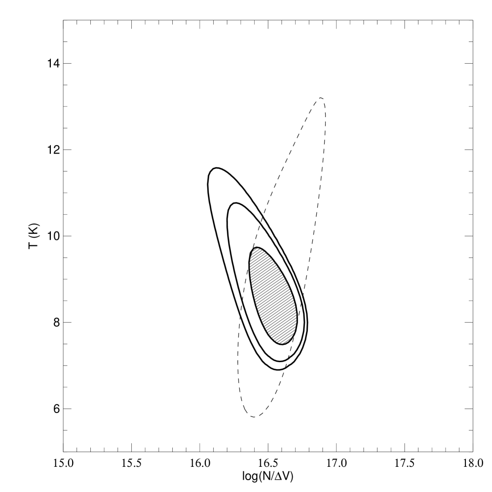
Figure 10.— Probability analysis of HLCs in (${{{\rm N}_{\rm\scriptscriptstyle CO}}}/\Delta V$)–temperature space, under LTE conditions (see Table 2). The dashed curve encloses the 1$\sigma$ confidence region when only HLC data for the (3–2) and lower transitions of ${}^{12}{\rm C}$O and ${}^{13}{\rm C}$O are taken into account. The solid contours enclose the 1,2, and 3$\sigma$ confidence intervals when the new (4–3)/(2–1) data (this paper) are included. The inner, 1$\sigma$, contour is shaded. The units of ${{{\rm N}_{\rm\scriptscriptstyle CO}}}/\Delta V$ are $\,{\rm cm}^{-2}\mkern-5.0mu$  $({\,{\,{\rm km}}{\,{\rm s}}^{-1}})^{-1}$.

4. Modelling the CO-emitting regions: A statistical approach

Here we introduce a statistical method for modelling the physical conditions in the CO-emitting cells of translucent molecular clouds. As stated above, integrated intensity ratios among the first four transitions of CO are constant. Define the following integrated intensity ratios for translucent clouds:

$$\frac{I_{(2-1)}}{I_{(1-0)}}\equiv(R_{1}\pm\sigma_{1}) = 0.77\pm 0.24;$$ (8)

$$\frac{I_{(3-2)}}{I_{(2-1)}}\equiv(R_{2}\pm\sigma_{2}) = 0.55\pm 0.16;$$ (9)

$$\frac{I_{(4-3)}}{I_{(2-1)}}\equiv(R_{3}\pm\sigma_{3}) = 0.11\pm 0.02;$$ (10)

$$\frac{I[^{13}{\rm CO}(1-0)]}{I[^{12}{\rm CO}(1-0)]}\equiv(R_{4}\pm\sigma_{4}) = 0.13\pm 0.04.$$ (11)

These ratios are taken from Equations 3, 4, 5, and 7. Suppose that fluctuations in the $i$th ratio, $r_{i}$, are distributed normally with mean $R_{i}$ and standard deviation $\sigma_{i}$. The probability of measuring the $i$th ratio to be between $r_{i}$ and $r_{i}+dr_{i}$ is then:

$$p(r_{i},R_{i},\sigma_{i})dr_{i}~{}=~{}\frac{1}{\sigma_{i}\sqrt{2\pi}}{\rm e}^{-(r_{i}-R_{i})^{2}/(2\sigma_{i}^{2})}\,dr_{i}.$$ (12)

Since the ratios are constant (excluding fluctuations), they are statistically independent of each other. The joint probability of observing a given set of ratios is thus given by the product:

$$P(r_{1},r_{2},r_{3},r_{4})dr_{1}dr_{2}dr_{3}dr_{4}\equiv P({\bf r})d{\bf r}=\prod_{i=1}^{4}p(r_{i},R_{i},\sigma_{i})dr_{i}.$$ (13)

This analysis requires that all the CO emission originates in gas with the same physical conditions. We of course have argued that this is the case (see §3.4). Therefore, given a physical model and an input grid of physical parameters, the line intensities, ${\rm T}_{\rm\scriptscriptstyle MB}\mkern-5.0mu$ , and ratios among them, $r$, can be computed. Equation 13 gives the probability distribution in the vector of ratios, r. This can be used to estimate the most likely portion of the input parameter space which gives the observed ratios. Below we evaluate the high density, low temperature (HDLT) and the low density, high temperature (LDHT) translucent cloud scenarios using two simple cloud models, the local thermodynamic equilibrium model and the large velocity gradient model.

4.0.1 The LTE model

In the HDLT scenario advocated by FP the CO emission originates in cold, high-density regions where the CO level populations are in local thermodynamic equilibrium (LTE). This scenario is worth investigating because of its extreme simplicity—in LTE the line ratios depend on only two parameters, the excitation temperature, ${\rm T_{\rm ex}}$, and the CO column density per velocity interval, ${\rm N}_{\rm\scriptscriptstyle CO}/{\Delta{\rm V}}$.

The peak intensity of a CO spectral line, ${\rm T}_{\rm\scriptscriptstyle MB}\mkern-5.0mu$ , is given in LTE by:

$${{{\rm T}_{\rm\scriptscriptstyle MB}}} = 5.53{\,{\rm K}}\,\left[\frac{1}{{\rm e}^{(5.53{\,{\rm K}})J/{{\rm T_{\rm ex}}}}-1}-\frac{1}{{\rm e}^{(5.53{\,{\rm K}})J/{\rm T_{BG}}}-1}\right]$$ (14)

$$(1-{\rm e}^{-\tau})\,\phi,$$

where ${\rm T_{\rm\scriptscriptstyle BG}}=2.7{\,{\rm K}}$ is the cosmic microwave background temperature and $\tau$ is the line center opacity. The transition is from rotational level $J$ to $J-1$. The function $\phi$ contains the details of the telescope beam average; if the emission originates from gas with uniform properties, then $\phi$ is simply the beam filling fraction of the gas. In this case, which we assume to hold for HLCs, $\phi$ cancels when line ratios are taken.

We will use the LTE model to predict ${\rm T}_{\rm\scriptscriptstyle MB}\mkern-5.0mu$  ratios, and then compare them directly with the observed $\int{{\rm T}_{\rm\scriptscriptstyle MB}}\,dV$ ratios (Equation 6) by assuming Gaussian line profiles. The LTE opacity for a transition from level $J$ to level $J-1$ is given by:

$$\tau_{J,J-1} = \frac{8\pi^{3}\mu^{2}}{3hZ({{\rm T_{\rm ex}}})}\,{\rm e}^{-(2.765{\,{\rm K}})J(J+1)/{{\rm T_{\rm ex}}}}$$ (15)

$$[{\rm e}^{(5.53{\,{\rm K}})J/{{\rm T_{\rm ex}}}}-1]\left[{{{\rm N}_{\rm\scriptscriptstyle CO}/{\Delta{\rm V}}}}\right]$$

$$\approx ~{}\frac{1.565\times 10^{-15}}{Z({{\rm T_{\rm ex}}})}\,\frac{[{\rm e}^{(5.53{\,{\rm K}})J/{{\rm T_{\rm ex}}}}-1]}{{\rm e}^{(2.765{\,{\rm K}})J(J+1)/{{\rm T_{\rm ex}}}}}$$

$$\left[\frac{{{{\rm N}_{\rm\scriptscriptstyle CO}/{\Delta{\rm V}}}}}{{\,{\rm cm}^{-2}}({\,{\,{\rm km}}{\,{\rm s}}^{-1}})^{-1}}\right].$$

Here $\mu=0.112\,$ debye is the electric dipole moment of the CO molecule and $Z({{\rm T_{\rm ex}}})$ is the CO rotational partition function:

$$Z({{\rm T_{\rm ex}}})~{}=~{}\sum_{J=0}^{\infty}(2J+1)\,\exp[-(2.765{\,{\rm K}})J(J+1)/{{\rm T_{\rm ex}}}].$$ (16)

Using a grid of values of ${\rm N}_{\rm\scriptscriptstyle CO}/{\Delta{\rm V}}$ and ${\rm T_{\rm ex}}$, we have computed the vector r of ratios under LTE conditions. The series in Equation 16 was truncated to 20 terms, since new terms added less than 1% to the value of $Z$. The ${}^{13}{\rm C}$O intensities were determined in the same way as the ${}^{12}{\rm C}$O intensities, except the ${}^{13}{\rm C}$O abundance was taken to be 1/60 that of ${}^{12}{\rm C}$O.

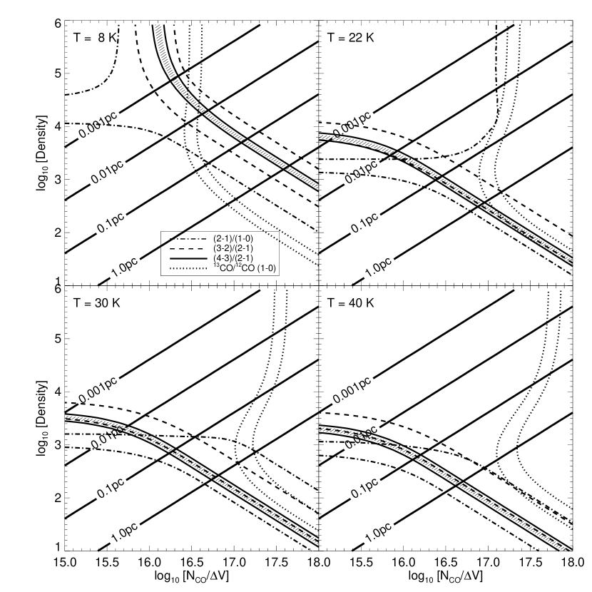
Figure 11.— Statistical equilibrium calculations for CO lines in clouds with a large velocity gradient (LVG). Each plot maps out observed cloud CO line ratios as a function of column density per unit velocity, ${{{\rm N}_{\rm\scriptscriptstyle CO}}}/\Delta V$, and gas volume density for a different temperature. The shaded region indicates the range of values of the ${}^{12}{\rm C}$O (4–3)/(2–1) ratio reported here for HLCs. Straight lines indicate the total “size” of the emitting regions, given by the ratio of column density to volume density, for CO-emitting cells with velocity width $\Delta V=1{\,{\,{\rm km}}{\,{\rm s}}^{-1}}$. The units of ${{{\rm N}_{\rm\scriptscriptstyle CO}}}/\Delta V$ are $\,{\rm cm}^{-2}\mkern-5.0mu$  $({\,{\,{\rm km}}{\,{\rm s}}^{-1}})^{-1}$. Density is in units of $\,{\rm cm}^{-3}\mkern-5.0mu$ .

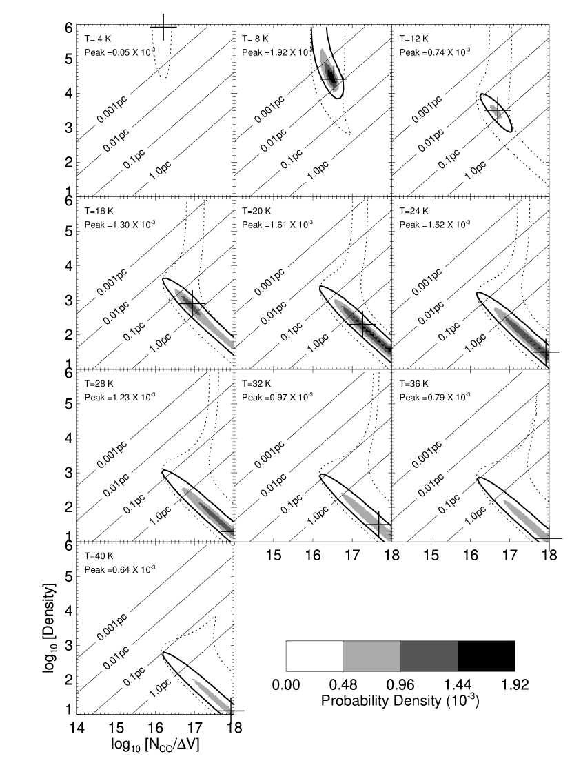
Figure 12.— The probability density field for HLC CO-emitting cells in the LVG model. Slices in the (${{{\rm N}_{\rm\scriptscriptstyle CO}}}/\Delta V$)–Density plane were made for 10 values of the temperature, and are represented as greyscale images. The dashed curves in each plot represent slices through the 3$\sigma$ confidence surface for the sample region of [${\rm T_{\rm k}}$, ${{{\rm N}_{\rm\scriptscriptstyle CO}}}/\Delta V$, $n$]–space when only HLC data for the (3–2) and lower transitions of ${}^{12}{\rm C}$O and ${}^{13}{\rm C}$O are taken into account. The solid contours represent slices through the 3$\sigma$ confidence surface when the new (4–3)/(2–1) data (this paper) are included. The crosses indicate the point in each slice where the probability density reaches its maximum value, listed as “Peak” on each graph. Straight lines indicate the “size” of the emitting regions, as described in Figure 11.

Predicted ${}^{12}{\rm C}$O LTE line ratios are listed in Table 2 as a function of excitation temperature for ${{{\rm N}_{\rm\scriptscriptstyle CO}}}=5\times 10^{16}{\,{\rm cm}^{-2}}$ and $\Delta V=1{\,{\,{\rm km}}{\,{\rm s}}^{-1}}$. The bottom row of the table gives the actual values observed towards HLCs. The measured (2–1)/(1–0), (3–2)/(2–1), and (4–3)/(2–1) ratios are all compatible with low temperatures, ${{\rm T_{\rm ex}}}\approx 5-10{\,{\rm K}}$. Using the probability distribution function, $P({\bf r})d{\bf r}$ (Equation 13), we can determine quantitatively a probability distribution in (${\rm N}_{\rm\scriptscriptstyle CO}/{\Delta{\rm V}}$, ${\rm T_{\rm ex}}$)–space. Figure 10 shows this. The dashed contour on the figure represents the 1$\sigma$ confidence interval (68.3% of the total probability) in the (${\rm N}_{\rm\scriptscriptstyle CO}/{\Delta{\rm V}}$, ${\rm T_{\rm ex}}$)–plane when only ratios 1, 2, and 4 are considered, i.e., when we neglect the new (4–3) data (this paper). The solid shaded contour represents the 1$\sigma$ confidence interval when the new data are included, and the two surrounding solid contours represent the 2 and 3$\sigma$ confidence intervals (95.4% and 99.7%, respectively, of the total probability). The new data have decreased the size of the 1$\sigma$ contour by a factor of $\sim 3$. The most probable set of physical properties is: ${{\rm T_{\rm ex}}}=(8.5\pm 1.5){\,{\rm K}}$ and ${{{\rm N}_{\rm\scriptscriptstyle CO}/{\Delta{\rm V}}}}={10^{16.5\pm 0.2}}{\,{\rm cm}^{-2}}\,({\,{\,{\rm km}}{\,{\rm s}}^{-1}})^{-1}$. Evidently, if CO-emitting regions are in LTE then the temperature is low, and the HDLT regime is the only solution. The LTE line center opacity (Equation 15) is $\tau=$ 9.6, 7.2, 2.1, and 0.3, for the ${}^{12}{\rm C}$O (1–0), (2–1), (3–2), and (4–3) transitions respectively. As we deduced from the observations (see Figure 9), the CO-emitting regions are optically thick to ${}^{12}{\rm C}$O (1–0) radiation. In fact, only the (4–3) and higher transitions of ${}^{12}{\rm C}$O are optically thin.

4.0.2 The LVG model

The LTE analysis is necessary but not sufficient to confirm the HDLT scenario because the LTE model does not consider the possibility of low density gas. We have simply shown that if the gas is dense enough such that the transitions are thermalized, then the temperature must be low. There is no reason a priori to believe this is true. If the temperature is high enough, intermediate levels such as $J=4$ may be significantly populated even in low density gas. Furthermore, it may be radiative trapping which causes the thermalization of level populations, rather than high densities. The LTE model cannot distinguish between such possibilities.

In this section we calculate the CO level populations in statistical equilibrium using the large velocity gradient (LVG) formalism (Sobolev 1960; Castor 1971). This approximation states that the mean free path of spectral line photons, $l_{\rm\scriptscriptstyle mfp}$, is on average much less than the product $\Delta V\,(dV/dR)^{-1}$, where $\Delta V$ is the total cloud velocity dispersion and $dV/dR$ is the cloud velocity gradient which is a systematic function of position. In the LVG approximation different regions in a cloud are effectively decoupled in velocity space, whence line radiation emitted from one region of the cloud does not interact with any other region. This simplifies considerably the radiative transfer computation.

Of course, the LVG approximation does not strictly hold in HLCs—it is unlikely that the velocity field in HLCs is so well-ordered as to produce a systematic velocity gradient. In general the clouds are not gravitationally bound (MBM; Keto & Myers 1986; Pound & Blitz 1993; Heithausen 1996), nor do they possess evidence of large–scale outflows or rotation (e.g., Pound et al. 1991). Instead, the velocity field in these clouds is most likely turbulent (Falgarone 1994; Falgarone et al. 1994), hence the velocity is a random function of position. Nevertheless, $l_{\rm\scriptscriptstyle mfp}$ is probably much less than the velocity correlation length of the turbulence, i.e., the spectral lines form under macro-turbulent conditions [see for example the simulations of Park & Hong (1995); see also the review in Falgarone et al. (1998)]. Macro-turbulence prevents distinct emission regions of a cloud from “shadowing” each other in velocity space, which is statistically equivalent to a large systematic velocity gradient in its effect on the radiative transfer through the cloud.

Since the level populations both determine and are determined by the radiation field, the solution of the equation of radiative transfer for CO line radiation with self-consistent level populations was performed numerically. The level populations in a statistical steady state, and the corresponding radiation field were computed for a grid of clouds, each with constant volume density, $n$, kinetic temperature, ${{\rm T_{\rm k}}}$, and CO abundance, ${\rm X}_{\rm\scriptscriptstyle CO}$. At the surface the incident radiation field was taken to be that due to the 2.7$\,{\rm K}\mkern-5.0mu$  cosmic microwave background. It was furthermore assumed that there is no internal radiation source in the clouds. Collisional rate coefficients for CO excitation by ${\rm H}_{2}\mkern-5.0mu$  were those computed by Flower & Launay (1985). A constant abundance ${{{\rm X}_{\rm\scriptscriptstyle CO}}}=8\times{10^{-5}}$ was assumed, i.e., in the CO-emitting regions approximately 80% of the carbon gas is in CO. This is based on the local ISM gas-phase carbon abundance which is observed to be [C]$=(1.4\pm 0.2)\times{10^{-4}}$ (Sofia, Cardelli, Guerin, & Meyer 1997). The results do not change drastically if ${\rm X}_{\rm\scriptscriptstyle CO}$ varies between 5 and 10 $\times{10^{-5}}$. The abundance of ${}^{13}{\rm C}$O was assumed to be 1/60 that of ${}^{12}{\rm C}$O, i.e., [${}^{13}{\rm C}$O]/[${}^{12}{\rm C}$O]=[${}^{13}{\rm C}$]/[${}^{12}{\rm C}$]. We have ignored the effects of chemical fractionation and isotope-selective photodissociation, which would cause the ${}^{13}{\rm C}$O/${}^{12}{\rm C}$O abundance ratio to range between 1/70 to 1/35 (§3.5; van Dishoeck & Black 1988).

The populations of the first eight rotational transitions of the ${}^{12}{\rm C}$O and ${}^{13}{\rm C}$O molecules were modelled. For each species the model was run for temperatures ranging from 4 to 40 K, for densities ranging from $10^{1}$ to $10^{6}$$\,{\rm cm}^{-3}\mkern-5.0mu$ , and for column density per velocity ranging from ${{{\rm N}_{\rm\scriptscriptstyle CO}/{\Delta{\rm V}}}}=10^{15}$ to $10^{18}$$\,{\rm cm}^{-2}\mkern-5.0mu$ /($\,{\,{\rm km}}{\,{\rm s}}^{-1}\mkern-5.0mu$ ). Results for ${\rm T_{\rm\scriptscriptstyle k}}=8$, 22, 30, and 40$\,{\rm K}\mkern-5.0mu$  are displayed in Figure 11. The observed range of values of the four ratios, $R_{i}\pm\sigma_{i}$ (defined in Equations 8 through 11), are indicated by pairs of contours. The range in the (4–3)/(2–1) ratio is shaded. For reference the size along the line-of-sight, $L$, of CO emitting regions is indicated by straight solid lines. A linewidth of $\Delta V=1{\,{\,{\rm km}}{\,{\rm s}}^{-1}}$ has been assumed, whence the following relationship gives the size:

$$\frac{L}{{\,{\rm pc}}}\approx 4.05\times{10^{-2}}\left(\frac{{{{\rm N}_{\rm\scriptscriptstyle CO}}}}{{10^{16}}{\,{\rm cm}^{-2}}}\right)\left(\frac{n}{{10^{3}}{\,{\rm cm}^{-3}}}\right)^{-1}\left[\frac{{{{\rm X}_{\rm\scriptscriptstyle CO}}}}{8{\times 10^{-5}}}\right]^{-1}.$$ (17)

Figure 12 shows the statistical analysis of the LVG results. Using the method described, we have computed the probability distribution function, $P({\bf r})d{\bf r}$, as a function of ${\rm N}_{\rm\scriptscriptstyle CO}/{\Delta{\rm V}}$, $n$, and ${\rm T_{\rm k}}$. The greyscale images in Figure 12 each represent a slice through the probability density field made in the (${\rm N}_{\rm\scriptscriptstyle CO}/{\Delta{\rm V}}$, $n$)–plane at a particular temperature. The dashed contour is a slice through the the 3$\sigma$ confidence surface if the (4–3)/(2–1) ratio is neglected and the solid contour represents a slice through the 3$\sigma$ confidence surface when the new data are included. The crosses indicate the point in the (${\rm N}_{\rm\scriptscriptstyle CO}/{\Delta{\rm V}}$, $n$)–plane where the probability density reaches its maximum value for the given temperature.

Figure 13.— Maximum-probability values of $P$, (${\rm N}_{\rm\scriptscriptstyle CO}/{\Delta{\rm V}}$), and $n$ in slices of constant ${\rm T_{\rm k}}$ (i.e., the values of the quantities at the crosses shown in Figure 12). Dashed curves represent these functions when only the (3–2) and lower transitions of CO are included, while solid curves include the new (4–3) data. The new data reduce the range of possible solutions, but do not alter significantly the most probable cloud conditions. Note that $P_{max}(T)$ is normalized so that the peak value equals unity. The absolute peak probability density value is 4 times higher for the current dataset than for the prior dataset.

The maximum probability density in each temperature slice, $P_{\rm max}({{\rm T_{\rm k}}})$, i.e., the value of the probability density at the location of the crosses, is printed on the plots. The probability field has two local maxima, one at ${{\rm T_{\rm k}}}\approx 8{\,{\rm K}}$ [$P_{\rm max}({{\rm T_{\rm k}}})=1.92\times{10^{-3}}$] and one at ${{\rm T_{\rm k}}}\approx 20{\,{\rm K}}\ [P_{\rm max}({{\rm T_{\rm k}}})=1.61\times{10^{-3}}]$. These correspond to the HDLT and LDHT solutions, respectively. The HDLT solution is the most probable. This regime is very well-defined in the (${\rm N}_{\rm\scriptscriptstyle CO}/{\Delta{\rm V}}$, $n$)–plane, with $n={10^{4.5\pm 0.5}}{\,{\rm cm}^{-3}}$, and ${{{\rm N}_{\rm\scriptscriptstyle CO}/{\Delta{\rm V}}}}={10^{16.6\pm 0.3}}{\,{\rm cm}^{-2}}({\,{\,{\rm km}}{\,{\rm s}}^{-1}})^{-1}$. It is reassuring that we get the same value of ${\rm N}_{\rm\scriptscriptstyle CO}/{\Delta{\rm V}}$ in the HDLT/LVG model as in the LTE model. The two models tell the same story: if the density is high then the level populations are thermalized in constant-opacity structures with ${{\rm T_{\rm k}}}\approx 8{\,{\rm K}}$. The ${}^{12}{\rm C}$O line center opacities in the LVG model are: $\tau=$ 9.6, 14.4, 6.3, and 1.0 for the (1–0), (2–1), (3–2), and (4–3) transitions, respectively. In this model all ${}^{12}{\rm C}$O radiation is produced in gas which is at least marginally optically thick.

As mentioned by FP the implied structure sizes in the HDLT case are very small, less than $\sim 0.01{\,{\rm pc}}$ ($\sim 2000\,$AU), which is consistent with the $<6500\,$AU–sized structures seen by Pound et al. (1991) in high–latitude cloud MBM-12. This HDLT structure size is $\lesssim$1% of the average projected CO size of HLCs ($\sim 1{\,{\rm pc}}$; Ingalls 1999). Thus in this interpretation a typical HLC is comprised of an ensemble of $\sim 10,000$ HDLT CO-emitting cells (given an area filling fraction of unity).

Unfortunately, it is still not possible to rule out the LDHT solution completely, since the probability field has a second local maximum at ${{\rm T_{\rm k}}}\approx 20{\,{\rm K}}$ which is about 80% as probable as the 8$\,{\rm K}\mkern-5.0mu$  maximum. We are, however, able to place a strict upper limit on the temperature in the CO-emitting regions due to the predicted size of LDHT structures. As mentioned in §1, the sizes of emitting structures along the line-of-sight (LOS) may be much larger than their sizes in the plane of the sky. It is not plausible, however, for LOS structure sizes to exceed the $\sim 1{\,{\rm pc}}$ cloud sizes. For very high temperatures (${{\rm T_{\rm k}}}\gtrsim 30{\,{\rm K}}$) the LOS size of emitting regions with nonzero probability in the model becomes unrealistically large. Unless most observed CO structures are filaments aligned along the line of sight, which is unlikely, temperatures greater than $\sim 30{\,{\rm K}}$ must be completely ruled out.

Again (see the LTE model) the ${}^{12}{\rm C}$O (4–3) data significantly decrease the size of the 3$\sigma$ surface in the parameter space. In other words, the range of possible solutions is decreased. Remarkably, including the higher transition data does not change the predicted physical conditions. We plot in Figure 13 the maximum-probability values of $P$, (${\rm N}_{\rm\scriptscriptstyle CO}/{\Delta{\rm V}}$), and $n$ (the values at the positions of the crosses). As for Figures 10 through 12, dashed curves represent these functions when only the (3–2) and lower transitions of CO are included, and solid curves represent the same functions when the new (4–3) data are used. Clearly the new data both limit the range of possible solutions in ${\rm T_{\rm k}}$-space (Figure 13, top) and also yield cloud conditions that are entirely consistent with those derived using the old data (Figure 13, middle and bottom).

5. Discussion

5.1. Physical Implications of HDLT Gas

We have studied the J = (1–0) through (4–3) transitions of CO in translucent clouds. Motivated by the work of Falgarone et al. (1991; 1992; 1998) and FP, instead of treating clouds as separate entities with distinct characteristics, we sought regularity in the CO emission. The linear relationships among the (1–0), (2–1), (3–2), and (4–3) transitions, as well as the constancy of the 60µm/100µm IRAS surface brightness ratio, justify this perspective. The simplest interpretation of these results is that the emission arises in regions with the same physical properties, or “cells”, and that variations in the emission are caused by variations in the beam filling fraction of the cells. We call this the “cell hypothesis”.

Two types of CO cell may exist: the low density, high temperature (LDHT) and the high density low temperature (HDLT) cell. The LDHT cell is relatively space-filling, with line of sight sizes of order 50% to 100% of the cloud size. It is also in thermal pressure equilibrium with the interstellar environment.

The existence of HDLT cells, on the other hand, is controversial. We have shown that cells with densities of order ${10^{4.5}}{\,{\rm cm}^{-3}}$ are the most probable source of CO emission. This challenges the picture of HLCs described by van Dishoeck et al. (1991), who argued against the possibility of gas with $n\sim{10^{4}}{\,{\rm cm}^{-3}}$. The HDLT scenario also defies one of the primary assumptions of interstellar physics, which holds that clouds are in hydrostatic equilibrium. HDLT cells have a thermal pressure $P/k\sim 2{\times 10^{5}}{\,{\rm cm}^{-3}}{\,{\rm K}}$, which is an order of magnitude greater than the ambient thermal ISM pressure. Is this a serious problem?

The interstellar medium is turbulent. Its structures are not the result of equilibrium processes. Recent simulations of magnetohydrodynamic (MHD) turbulence performed by Ballesteros-Paredes, Vásquez-Semadeni, & Scalo (1999) show that thermal pressure equilibrium is irrelevant, since in MHD turbulence the volume and surface terms of the Eulerian Virial Theorem are comparable. As a consequence, structures will nearly always deform under inertial motions, resulting in “clumping” on many scales. According to this model, in a turbulent cloud, clumps are continually forming due to density fluctuations and dissipating due to radiative cooling. Quasi-static configurations are highly unlikely, unless compressed to sizes $L\lesssim 0.01{\,{\rm pc}}$, where self-gravity becomes important. Ironically, the HDLT cells are approximately this size. If the simulations of Ballesteros-Paredes et al. (1999) are correct, then the only stable configuration in translucent molecular clouds is the HDLT one. This important result needs to be confirmed. Is the CO emission produced only in stable structures which are in LTE? This would explain the remarkable uniformity we see in the CO line ratios for a large sample of clouds.

5.2. Limitations of the Method

We have attempted in this paper to evaluate two competing models for the physical state of molecular gas in translucent clouds, the HDLT and LDHT models. Both van Dishoeck et al. (1991) and FP state that neither HDLT nor LDHT conditions uniquely describe the data (even though each group concludes by favoring a different configuration; see §1). We have assumed that clouds are macro-turbulent, and we have argued that the LVG radiative transfer model is an adequate approximation of macro-turbulence. By deriving a probability density field in the physical parameter space we have shown quantitatively that HDLT gas is the more likely source of observed CO emission.

Our analysis is limited, however, by the extent to which the LVG scenario is an accurate representation of the velocity field of translucent gas. The assumption that clouds are macro-turbulent is based on the extensive three-dimensional radiative transfer simulations done by Park & Hong (1995). Nevertheless, it can be argued that using the macro-turbulent LVG assumption has biased our results in favor of HDLT conditions, since tiny HDLT cells are more likely to satisfy the LVG criterion, because they are less likely to shadow each other along the line of sight than the much larger ($\sim 0.5-1\,$pc) LDHT cells. Furthermore, since they have larger values of ${{{\rm N}_{\rm\scriptscriptstyle CO}}}/\Delta V$, LDHT cells have a much larger column density of radiatively coupled gas than HDLT cells with the same internal velocity dispersion. Thus the macro-turbulent approximation should break down for the largest LDHT cells. A more complete study would vary the statistics of the velocity field between the micro-turbulent and macro-turbulent limits. This is beyond the scope of the current paper, and we leave it to future work.

5.3. Testing for HDLT Cells

If HDLT cells exist, then they can be detected directly in CO emission using a millimeter-wave interferometer. A resolved HDLT cell would have a Rayleigh-Jeans brightness temperature in ${}^{12}{\rm C}$O (1–0) of ${{\rm T}_{\rm\scriptscriptstyle A}}\approx 5{\,{\rm K}}$. An interferometer with a spatial resolution of 0.001$\,{\rm pc}\mkern-5.0mu$  (for a cloud at a distance of 100$\,{\rm pc}\mkern-5.0mu$  this corresponds to an angular resolution of 2″) would be able to detect such HDLT cells. If there is no detectable ${}^{12}{\rm C}$O (1–0) emission in HLCs at 2″ scales, then the HDLT hypothesis is false.

References

- (1) Ballesteros-Paredes, J., Vásquez-Semadeni, E., & Scalo, J. 1999, ApJ, 515, 296
- (2) Bennett, C. L. et al. 1994, ApJ, 436, 423
- (3) Boreiko, R. T. & Betz, A. L. 1996, ApJ, 467, L113
- (4) Castor, J. I. 1970, MNRAS, 149, 111
- (5) Chamberlin, R. A., Lane, A. P., & Stark, A. A. 1997, ApJ, 476, 428
- (6) Chiar, J. E., Kutner, M. L., Verter, F., & Leous, J. 1994, ApJ, 431, 658
- (7) Clemens, D. P. & Barvainis, R. 1988, ApJS, 68, 257
- (8) Dame, T. M., Elmegreen, B. G., Cohen, R. S., & Thaddeus, P. 1986, ApJ, 305
- (9) Désert, F. -X., Boulanger, F., & Puget, J. L. 1990, A&A, 237, 215
- (10) Draine, B. T. 1978, ApJS, 36, 595
- (11) Dwek, E. et al. 1997, ApJ, 475, 565
- (12) Erickson, N.R., Goldsmith, P.F., Novak, G., Grosslein, R.M., Viscuso, P.J., Erickson, R.B., & Predmore, C.R. 1992, IEEE Trans. on Microwave Theory and Techniques, 40, 1
- (13) Falgarone, E., Panis, J. -F., Heithausen, A., Pérault, M., Stutzki, J., Pugent, J. -L., & Bensch, F. 1998, A&A, 331, 669
- (14) Falgarone, E. 1994, in The First Symposium on the Infrared Cirrus and Diffuse Interstellar Clouds, eds R.M. Cutri and W.B. Latter (San Francisco: ASP), 368
- (15) Falgarone, E. & Phillips, T. G. 1996, ApJ, 472, 191 (FP)
- (16) Falgarone, E., Phillips, T. G., & Walker, C. K. 1991, ApJ, 378, 186
- (17) Falgarone, E., Puget, J.-L., & Pérault, M. 1992, A&A, 257, 715
- (18) Flower, D. R. & Launay, J. M. 1985, MNRAS, 214, 271
- (19) Habing, H. J. 1968, Bull. Astron. Inst. Netherlands, 19, 421
- (20) Handa, T., Hasegawa, T., Hayashi, M., Sakamoto, S., Oka, T., & Dame, T. 1993, in Back to the Galaxy, ed S. S. Holt & F. Verter (AIP Conf Proc), 315
- (21) Heithausen, A. 1996, A&A, 314, 251
- (22) Heithausen, A., Bensch, F., Stutzki, J., Falgarone, E., & Panis, J. -F. 1998, A&A, 331, L65
- (23) Heithausen, A., Corneilussen, U., & Grossman, V. 1998, A&A, 330, 311
- (24) Ingalls, J. G. 1999, PhD Thesis, Boston University
- (25) Ingalls, J. G., Bania, T. M., & Jackson, J. M. 1994, ApJ, 431, L139
- (26) Ingalls, J. G., Chamberlin, R. A., Bania, T. M., Jackson, J. M., Lane, A. P., & Stark, A. A. 1997, ApJ, 479, 296
- (27) IRAS Catalogs & Atlases: Explanatory Supplement 1988, eds C. A. Beichman, G. Neugebauer, H.J. Habing, P.E. Clegg, & T.J. Chester (Washington, DC: GPO)
- (28) Keto, E. R., & Myers, P. C. 1986, ApJ, 304, 466
- (29) Langer, W. D., & Penzias, A. A. 1993, ApJ, 408, 539
- (30) Ladd, N., & Heyer, M. 1996, Characterization of the FCRAO 14-m Telescope with QUARRY (FCRAO Technical Memorandum 28 October 1996)
- (31) Levine, D. A. et al. 1993, IPAC User’s Guide, 5th ed., (Pasadena, CA: California Institute of Technology)
- (32) Low, F. J., et al. 1984, ApJ, 278, L19
- (33) Magnani, L., Blitz, L., & Mundy, L. 1985 ApJ, 295, 402 (MBM)
- (34) Magnani, L., Caillault, J.-P., Buchalter, A., & Beichman, C. A. 1995, ApJS, 96, 159
- (35) Magnani, L., Hartmann, D., & Speck, B. G. 1996 ApJS, 106, 447
- (36) Marscher, A. P., Moore, E. M., & Bania, T. M. 1993, ApJ, 419, L101
- (37) Park, Y. -S. & Hong, S. S. 1995, A&A, 300, 890
- (38) Pound, M. W. 1996, ApJ, 457, L35
- (39) Pound, M. W., Bania, T. M., & Wilson, R. W. 1990, ApJ, 351, 165
- (40) Pound, M. W. & Blitz, L. 1993, ApJ, 418, 328
- (41) Reach, W. T., Pound, M. W., Wilner, D. J., & Lee, Y. 1995, ApJ, 441, 224
- (42) Sanders, D. B., Scoville, N. Z., Tilanus, R. P. J., Wang, Z., & Zhou, S. 1993, in Back to the Galaxy, ed S. S. Holt & F. Verter (AIP Conf Proc), 311
- (43) Sanders, D. B., Clemens, D. P., Scoville, N. Z., & Solomon, P. M. 1986, ApJS, 60, 1
- (44) Schieder, R., Tolls, V., & Winnewisser, G. 1989, Experimental Astronomy, 1, 101
- (45) Sobolev, V. V. 1960, Moving Envelopes of Stars (Cambridge: Harvard University Press)
- (46) Sofia, U. J., Cardelli, J. A., Guerin, K. P., & Meyer, D. M. 1997, ApJ, 482, L105
- (47) Stark, A. A., Chamberlin, R. A., Ingalls, J. G., Cheng, J., Wright, G. 1997, Rev. Sci. Inst., 68(5), 2200
- (48) Stark, R., & van Dishoeck, E. F. 1994, A&A, 286, L43
- (49) Stark, R., 1995, A&A, 301, 873
- (50) Taylor, J. R. 1997, An Introduction to Error Analysis, 2nd edition, (Sausalito, CA: University Science Books), p 291
- (51) Tielens, A. G. G. M., & Hollenbach, D. 1985, ApJ, 291, 722
- (52) Turner, B. E. 1994, in The First Symposium on the Infrared Cirrus and Diffuse Interstellar Clouds, ed. R. M. Cutri and W. B. Latter (ASP Conf Ser 58), 307
- (53) Turner, B. E., Terzieva, R., & Herbst, E. 1999, ApJ, 518, 699
- (54) van Dishoeck, E. F., & Black, J. H. 1988, ApJ, 334, 771
- (55) van Dishoeck, E. F., Black, J. H., Phillips, T. G., & Gredel, R. 1991, ApJ, 366, 141
- (56) Wright, E. L. et al. 1991, ApJ, 381, 200