Non-linear Stochastic Galaxy Biasing in Cosmological Simulations

Abstract

We study the biasing relation between dark-matter halos or galaxies and the underlying mass distribution, using cosmological $N$-body simulations in which galaxies are modelled via semi-analytic recipes. The nonlinear, stochastic biasing is quantified in terms of the mean biasing function and the scatter about it as a function of time, scale and object properties. The biasing of galaxies and halos shows a general similarity and a characteristic shape, with no galaxies in deep voids and a steep slope in moderately underdense regions. At $\sim 8\mbox{$h^{-1}$ Mpc}$, the nonlinearity is typically $\lower 2.15277pt\hbox{$\;\buildrel<\over{\sim}\;$}10$ percent and the stochasticity is a few tens of percent, corresponding to $\sim 30$ percent variations in the cosmological parameter $\beta=\Omega^{0.6}/b$. Biasing depends weakly on halo mass, galaxy luminosity, and scale. The observed trend with luminosity is reproduced when dust extinction is included. The time evolution is rapid, with the mean biasing larger by a factor of a few at $z\sim 3$ compared to $z=0$, and with a minimum for the nonlinearity and stochasticity at an intermediate redshift. Biasing today is a weak function of the cosmological model, reflecting the weak dependence on the power-spectrum shape, but the time evolution is more cosmology-dependent, relecting the effect of the growth rate. We provide predictions for the relative biasing of galaxies of different type and color, to be compared with upcoming large redshift surveys. Analytic models in which the number of objects is conserved underestimate the evolution of biasing, while models that explicitly account for merging provide a good description of the biasing of halos and its evolution, suggesting that merging is a crucial element in the evolution of biasing.

1 Introduction

The standard picture of the growth of structure via gravitational instability within a dark-matter dominated universe has led to a successful and predictive theoretical framework. However, in order to make direct contact with most observations, the relationship between galaxies and the underlying dark-matter distribution must be understood. This relationship has come to be loosely referred to as galaxy “biasing” [Davis et al. (1985), Bardeen et al. (1986), Dekel & Rees (1987)].

Given the complexity of the process of galaxy formation, it would be surprising if the galaxy distribution traced the mass distribution in a simple way. Various physical mechanisms have been proposed that could lead to galaxy biasing, but the features of the biasing process remain highly uncertain, including, for example, non-linearity, scale dependence, and stochasticity. Even the direction of the biasing, i.e. bias or anti-bias, is sometimes uncertain.

Yet, there are many observational indications that galaxy biasing does exist and is non-trivial; for example, the dependence of galaxy clustering on type or environment [Dressler (1980), Hermit et al. (1996), Willmer et al. (1998), Tegmark & Bromley (1998)], or the evolution of biasing in time [Steidel et al. (1998), Adelberger et al. (1998)]. To the extent that the cosmological parameters are known, studying galaxy biasing will allow us to better understand the process of galaxy formation. Conversely, better understanding of biasing is a crucial component in interpreting the results of methods that attempt to use galaxies as tracers of the underlying density field and thus determine the cosmological density parameter $\Omega$ (see reviews by [Strauss & Willick (1995)], [Dekel (1994)], [Dekel et al. (1997)], and [Dekel (1999)]).

Modern $N$-body techniques have provided the basis for a great deal of progress in understanding the clustering of dark-matter halos relative to the underlying matter density field (e.g. [Gross et al. (1998)], [Jenkins et al. (1998)]). Analytic approximations based within the hierarchical-merger framework have led to additional insights (e.g. [Mo & White (1996)] and extensions, cf. [Catelan et al. (1998)]). However, these halos do not necessarily correspond to galaxies. One reason for this is the “over-merging” problem: dark matter halos that are incorporated within a larger collapsed structure may lose their identities due to the limited numerical resolution of the simulation. In addition, the biasing properties of the halos include only the effects of clustering due to gravity and do not reflect the astrophysical processes involving gas and stars, which are presumably important in determining the properties of real galaxies.

Recent theoretical studies have used a variety of techniques to address these issues. For example, ?), ?) ?) and ?) used cosmological simulations with hydrodynamics and phenomenological recipes for star formation. ?) used very high-resolution dissipationless N-body simulations, in which the over-merging problem is largely overcome and there should be a good one-to-one correspondence between dark matter halos and galaxies. ?) and ?) used various “toy models” to describe galaxy formation in large, low resolution dissipationless N-body simulations. ?) and ?) used semi-analytic techniques to assign galaxies to halos within dissipationless N-body simulations.

All of these techniques have certain advantages and disadvantages. The present study provides a useful complement to this previous work, and is unique in several respects. We model galaxies using a new technique [Kauffmann et al. (1998a)], in which $N$-body simulations are combined with semi-analytic modelling of galaxy formation. Merging histories of dark matter halos (hereafter referred to simply as halos) are extracted from large dissipationless N-body simulations using the outputs at finely spaced time steps. Within the framework of these “merger trees”, gas dynamics, star formation, supernovae feedback, and galaxy merging are modelled semi-analytically. The results are convolved with stellar population models. In this way, we obtain predictions of observable galaxy properties such as magnitudes, colours, star formation rates, and morphologies. This allows us to study the dependence of galaxy biasing on these characteristics at different cosmological epochs and at different smoothing scales. Another novel aspect of this work is that we utilize the biasing formalism developed by ?), which allows us to separate and quantify the nonlinearity and the stochasticity of the biasing relation.

The outline of the paper is as follows. In Section 2, we summarize the biasing formalism and analytic models for halo biasing. In Section 3, we briefly describe the simulations and the semi-analytic techniques used to model galaxy formation. In Section 4, we discuss the relationship between the halos and galaxies in our simulations. In Section 5, we study the dependence of the biasing relation on halo mass, galaxy luminosity and type, scale, and redshift. In Section 6, we compare the results of the simulations with analytic models of biasing. We summarize our results and conclude in Section 7.

2 Descriptions and Models of Biasing

A biasing scheme relates the density fluctuation fields of galaxies and mass. For the mass, we define $\delta(\vec{x})\equiv[\rho(\vec{x})-\rho_{\rm b}]/\rho_{\rm b}$, where $\rho_{\rm b}$ is the background density. We denote the corresponding fields for the galaxies (or halos) by $\delta_{\rm g}(\vec{x})$. The two fields are smoothed with the same window function of scale $R_{\rm s}$. We assume that biasing is a local process, which means that the galaxy density field $\delta_{\rm g}$ is related to $\delta$ within the local smoothing volume.

2.1 Descriptions of Non-linear, Stochastic Biasing

The simplest possible model for biasing is strictly linear and deterministic:

$$\delta_{\rm g}(\vec{x})=b\,\delta(\vec{x}).$$ (1)

A less restrictive definition of linear biasing follows from the theory of biasing of density peaks in a Gaussian random field [Kaiser (1984), Bardeen et al. (1986)], which predicts that the galaxy-galaxy and matter-matter correlation functions are related in the linear regime by a constant multiplicative factor,

$$\xi_{\rm gg}(r)=b^{2}\xi_{\rm mm}(r).$$ (2)

In both cases, $b$ is referred to as the “linear biasing parameter”. Eqn. 2 follows from Eqn. 1 but the converse is not true.

Linear deterministic bias can serve only as a crude null hypothesis: it is not a self-consistent model, it has no theoretical motivation and it seems inconsistent with observations. ?, hereafter DL) have proposed a general formalism for non-linear, stochastic local biasing, which we shall adopt in this paper. We shall denote the one-point probability distribution functions (PDF) for the matter and galaxy density fields as $P(\delta)$ and $P(\delta_{\rm g})$. By definition, both distributions have zero mean, and the corresponding variances are $\sigma^{2}\equiv\langle\delta^{2}\rangle$ and $\sigma_{\rm g}^{2}\equiv\langle\delta_{\rm g}^{2}\rangle$. The local biasing relation between galaxies and matter is treated as a non-deterministic process, specified by the conditional biasing distribution $P(\delta_{\rm g}|\delta)$. The mean biasing function $b(\delta)$ is then defined by

$$b(\delta)\delta\equiv\langle\delta_{\rm g}|\delta\rangle=\int d\delta_{\rm g}\,P(\delta_{\rm g}|\delta)\,\delta_{\rm g}.$$ (3)

This function fully characterizes the mean non-linear biasing and reduces naturally to the linear biasing relation Eqn. 1 if $b$ is independent of $\delta$.

Useful statistics for characterizing the mean biasing and its non-linearity are the moments

$$\hat{b}\equiv\langle b(\delta)\delta^{2}\rangle/\sigma^{2}$$ (4)

and

$$\tilde{b}^{2}\equiv\langle b^{2}(\delta)\delta^{2}\rangle/\sigma^{2}.$$ (5)

To describe the statistical nature of the biasing relation, we define the random biasing field

$$\epsilon=g-\langle\delta_{\rm g}|\delta\rangle,$$ (6)

and its variance, the biasing scatter function

$$\sigma^{2}_{b}(\delta)\equiv\langle\epsilon^{2}|\delta\rangle/\sigma^{2}.$$ (7)

Averaging over $\delta$, one obtains the biasing scatter $\sigma_{\rm b}$:

$$\sigma^{2}_{\rm b}\equiv\langle\epsilon^{2}\rangle/\sigma^{2}.$$ (8)

To second order, the three parameters $\hat{b}$, $\tilde{b}$ and $\sigma_{\rm b}$ characterize any local, non-linear and stochastic biasing relation. The parameter $\hat{b}$ is simply the slope of the linear regression of $\delta_{\rm g}$ on $\delta$, and as such it is a natural generalization of the linear biasing parameter of Eqn. 1. The ratio $\tilde{b}/\hat{b}$ quantifies the non-linearity of the mean biasing relation and $\sigma_{\rm b}/\hat{b}$ independently measures the scatter. Thus the non-linearity and stochasticity can be studied separately. The formalism reduces in a natural way to linear biasing when $\tilde{b}=\hat{b}$ and to deterministic biasing when $\sigma_{\rm b}=0$. We do not investigate moments higher than second order in this paper, but the formalism is readily generalizable.

Various statistics describing biasing are used in the literature and commonly referred to without distinction as “the” bias parameter. In general, these statistics are not equivalent. Here we follow the notation of DL which naturally generalizes the linear deterministic biasing parameter of Eqn. 1 into the mean biasing parameter $\hat{b}$ of Eqn. 4. The biasing parameter relating the variances at a given smoothing scale is denoted $b_{\rm var}$, and it can be expressed in terms of the three basic parameters above:

$$b_{\rm var}\equiv{\sigma_{g}\over\sigma}=\hat{b}\left[\frac{\tilde{b}^{2}}{\hat{b}^{2}}+\frac{\sigma_{b}^{2}}{\hat{b}^{2}}\right]^{1/2}\,.$$ (9)

A complementary parameter is the linear correlation coefficient

$$r\equiv\frac{\langle\delta_{\rm g}\delta\rangle}{\sigma_{\rm g}\sigma}=\left[\frac{\tilde{b}^{2}}{\hat{b}^{2}}+\frac{\sigma_{b}^{2}}{\hat{b}^{2}}\right]^{-1/2}\,.$$ (10)

Note that both $b_{\rm var}$ and $r$ mix nonlinear and stochastic effects. We denote the ratio of correlation functions at a given separation by $b_{\xi}=\sqrt{\xi_{\rm gg}/\xi_{\rm mm}}$.

2.2 Models of Biasing

2.2.1 Galaxy Conserving Models

The bias and linear correlation coefficient are expected to evolve with time in accord with the evolution of clustering. If the galaxies behave as test particles in the matter density field and their numbers and intrinsic properties are conserved, then they satisfy the continuity equation $\dot{\delta_{\rm g}}\simeq\dot{\delta}\simeq-\nabla\cdot v$. The parameters $b_{\rm var}$ and $r$ then evolve as [Tegmark & Peebles (1998)]:

$${b}_{0} = [(1-D)^{2}+2D(1-D)br+D^{2}b^{2}]^{1/2}$$ (11)

$$r_{0} = [(1-D)+Dbr]/{b}_{0}\,,$$ (12)

where $b_{0}$ and $r_{0}$ are the present day quantities, $b$ and $r$ are the corresponding values at some earlier redshift $z$, and $D$ is the linear growth factor at $z$ (normalized to unity today). If there is no correlation between galaxies and mass ($r=1$), this expression reduces to the model originally proposed by ?). We shall refer to this type of model as “galaxy conserving” (GC).

2.2.2 Hierarchical Merging Models

?, hereafter MW) developed a model for the biasing of virialized dark-matter halos with respect to the underlying matter distribution. Their model is based on an extension of the Press-Schechter approximation [Press & Schechter (1974)], and accounts for halo merging and continuous formation of new halos. They derived an expression for the mean nonlinear biasing function $b(\delta;M,z,R_{s})$ of halos with mass $M$ at a redshift $z$ for a smoothing scale $R_{s}$ (MW eqn. 19-20). In the vicinity of $|\delta|\gg\delta_{1}$, where $\delta_{1}\equiv\delta_{c}(1+z)$ is the density of a collapsed object, this reduces to the simple linear biasing factor:

$$b(M,z)=1+\frac{\nu^{2}-1}{\delta_{1}}\,,$$ (13)

where $\nu\equiv\delta_{1}/\sigma(M)$, and $\sigma(M)$ is the rms mass variance. MW showed that their model predictions for these quantities are in good agreement with the results of N-body simulations with scale-free initial power spectra, $P(k)\propto k^{n}$.

2.2.3 Shot Noise and Stochasticity

In empirical measures of the scatter in the biasing relation, shot noise is inevitably mixed with the physical sources of stochasticity. Removing this shot noise is not straightforward because halos or galaxies correspond to rare peaks in the density distribution, and their selection is far from a Poisson process. Let us imagine however a deterministic biasing scheme with a known form $\langle\delta_{\rm g}|\delta\rangle$ (for example, measured from a simulation). The expected variance in the number of galaxies $N$ in a smoothing window with volume $V$ and overdensity $\delta$ is $\mu_{2}\equiv\langle(N-\langle N\rangle)^{2}\rangle=N=nV(1+\delta_{\rm g})$, where $n$ is the global average number density of galaxies. The variance of the galaxy field $\delta_{\rm g}$ as a function of $\delta$ is then $\sigma^{2}_{g}(\delta)=\mu_{2}/(nV)^{2}=(1+\delta_{\rm g}(\delta))/(nV)$. We shall refer to this simple model as the “conditional Poisson” model.

3 Simulations

The dissipationless $N$-body simulations and the semi-analytic method used to model galaxies within these simulations are described in detail in ?). Here, we briefly summarize only their main features.

3.1 $N$-body Simulations

Table 2: Simulation Parameters. From left to right: the cosmological mass-density parameter $\Omega$, the Hubble constant $h\equiv H_{0}/(100\,\mbox{km s${}^{-1}$ Mpc${}^{-1}$})$, the linear rms mass density in a sphere of radius $8\mbox{$h^{-1}$ Mpc}$ $\sigma_{8}$, the box size $L$, and the mass per particle, $m_{\rm p}$.

Model	$\Omega$	$h$	$\sigma_{8}$	$L$ ($h^{-1}$ Mpc)	$m_{\rm p}$ ($h^{-1}$ $M_{\odot}$)
$\tau$CDM	1.0	0.5	0.6	85	$1.0\times 10^{10}$
$\Lambda$CDM	0.3	0.7	0.90	141	$1.4\times 10^{10}$

Special $N$-body simulations were run for this project (termed “GIF”) using the version of the adaptive particle-particle particle-mesh (AP³M) Hydra code developed as part of the VIRGO supercomputing project. The simulations have $N_{\rm p}=256^{3}$ particles and 512 cells on a side, and a gravitational softening length of $30\mbox{$h^{-1}$ kpc}$ ($h\equiv H_{0}/(100\,{\rm km\,s^{-1}\,Mpc^{-1}})$). Here we analyze only two of the four cosmological models simulated for the GIF project (see Table 2). One model, $\tau$CDM, has $\Omega=1$ and the other, $\Lambda$CDM, has $\Omega=0.3$ and a cosmological constant $\Omega_{\Lambda}=0.7$. The initial power spectra of fluctuations both have a shape parameter $\Gamma=0.21$ and are normalized to approximately reproduce the number density of clusters at the present epoch. Dark matter halos were identified using a standard friends-of-friends algorithm with a linking length 0.2 times the mean interparticle separation, thus corresponding to a density contrast of $\sim 125$ at the outer parts of the halos. We do not include any halos smaller than 10 particles in our analysis, as tests show that these halos are not stable over many output times.

3.2 Semi-Analytic Modelling of Galaxies

A “merger tree” is constructed for each halo identified at $z=0$ by searching for its progenitor halos at earlier redshifts. A halo at an early redshift $z_{1}$ is defined to be a progenitor of a halo at a later redshift $z_{0}<z_{1}$ if more than half of the particles of the progenitor and its most-bound particle are included in the halo at $z_{0}$. The progenitors are the halos that will merge together to form the parent halo at $z=0$. If a halo is at the top level of the hierarchy (i.e. it has no progenitor with at least 10 particles), then it is assumed to contain hot gas at the virial temperature of the halo. This gas is allowed to cool according to the radiative cooling timescale, and the cold gas is assumed to settle into a galactic disk and form stars.

The star formation rate is given by the expression

$$\dot{m}_{*}=\alpha\>\frac{m_{\rm cold}}{t_{\rm dyn}},$$ (14)

where $\alpha$ is a free parameter, $m_{\rm cold}$ is the mass of cold gas in the disk, and $t_{\rm dyn}$ is the dynamical time of the disk. The dynamical time is approximated as $t_{\rm dyn}=0.1r_{\rm vir}/V_{c}$, where $r_{\rm vir}$ is the virial radius and $V_{c}$ is the circular velocity of the halo at $r_{\rm vir}$. Cold gas may be reheated by supernovae feedback, with the rate of reheating given by the expression

$$\dot{m}_{\rm rh}=\epsilon\left(\frac{V_{0}}{V_{c}}\right)^{2}\dot{m}_{*},$$ (15)

where $\epsilon$ is a free parameter, and $V_{0}$ is a scaling constant. Reheated gas is removed from the cold gas reservoir. It may then be retained in the halo where it will cool again on a relatively short time scale, or ejected from the halo. If ejected, the gas is returned to the halo after the mass of the halo has grown by a factor of two or more.

The N-body simulations used here do not have sufficient resolution to resolve sub-halos once they are incorporated into larger halos. Therefore, the merging rate of galaxies within the halos is modeled semi-analytically. When halos merge, the central galaxy of the largest progenitor halo becomes the central galaxy of the new halo and all other galaxies become “satellite” galaxies. A satellite galaxy is assumed to merge with the central galaxy once its dynamical friction timescale has elapsed (see [Binney & Tremaine (1987)]). The morphologies of the galaxies are determined by assuming that major mergers ($m_{\rm sat}/m_{\rm central}>0.3)$ result in destruction of the disk and consumption of all remaining gas in a starburst. The remnant is assumed to be a bare spheroid. Subsequent gas cooling may result in the formation of a new disk. The bulge-to-disk ratio at each output redshift is then used to divide the galaxies into rough morphological categories.

The star formation history of each galaxy is convolved with stellar population synthesis models to obtain total luminosities in any desired filter band. The models of ?) are used, assuming that all stars have solar metallicity, and a standard Scalo initial mass function [Scalo (1986)]. The effects of dust extinction on the galaxy spectra were investigated using the empirical recipe of ?) (WH), in which the face-on optical depth in the B-band is parameterized in the form:

$$\tau_{B}\propto\tau^{*}_{B}(L_{B}/L_{B}^{*})^{\beta}\,,$$ (16)

with $\beta=0.5$, $\tau^{*}_{B}=0.8$, and $L_{B}=1.3\times 10^{10}h^{-2}L_{\odot}$. This can be extended to other wavebands using a standard Galactic extinction curve. The extinction is then computed by assigning a random inclination to each galaxy and using a standard “slab” model (see ?) for details).

The two free parameters in the galaxy formation models ($\alpha$ in Eqn. 14 and $\epsilon$ in Eqn. 15) are set by requiring the central galaxy in a halo with $V_{c}=220\,\mbox{km s${}^{-1}$}$ at the present epoch to have an I-band magnitude of $M_{I}-5\log h\sim-22.1$ and a cold gas mass of $m_{\rm cold}\sim 10^{10}\mbox{$M_{\odot}$}$. This ensures that the zero-point of the Tully-Fisher relation for spiral galaxies is in agreement with observations (e.g. [Giovanelli et al. (1997)]).

Various properties of the galaxies produced using these techniques are summarized in the companion papers based on the GIF simulations, ?), ?), and ?). We note that throughout this paper, we include in our analysis only galaxies that reside in halos of least 10 particles.

4 From Halos to Galaxies

The study of biasing is in some sense the attempt to understand the connection between the total mass density, which we believe to be dominated by dark matter, and the density of luminous galaxies. A fairly robust component of modern galaxy formation theory is that galaxies form within collapsed, virialized dark-matter halos. The clustering properties of these halos relative to the underlying mass distribution are straightforward to compute from cosmological $N$-body simulations such as the ones that we have described, subject only to the numerical limitations of the simulation at hand. Predicting how these halos are connected to visible galaxies is far more difficult. We have adopted the particular recipes described above, but other equally plausible recipes could lead to different results. In this section we quantify the resulting statistical relation between halos and galaxies in our simulations, and in the next section we present in parallel the results for the biasing properties of halos and galaxies. In this way we hope to gain some insight into the extent to which the biasing of galaxies is determined by the gravitational process of halo formation and to what extent by other astrophysical processes.

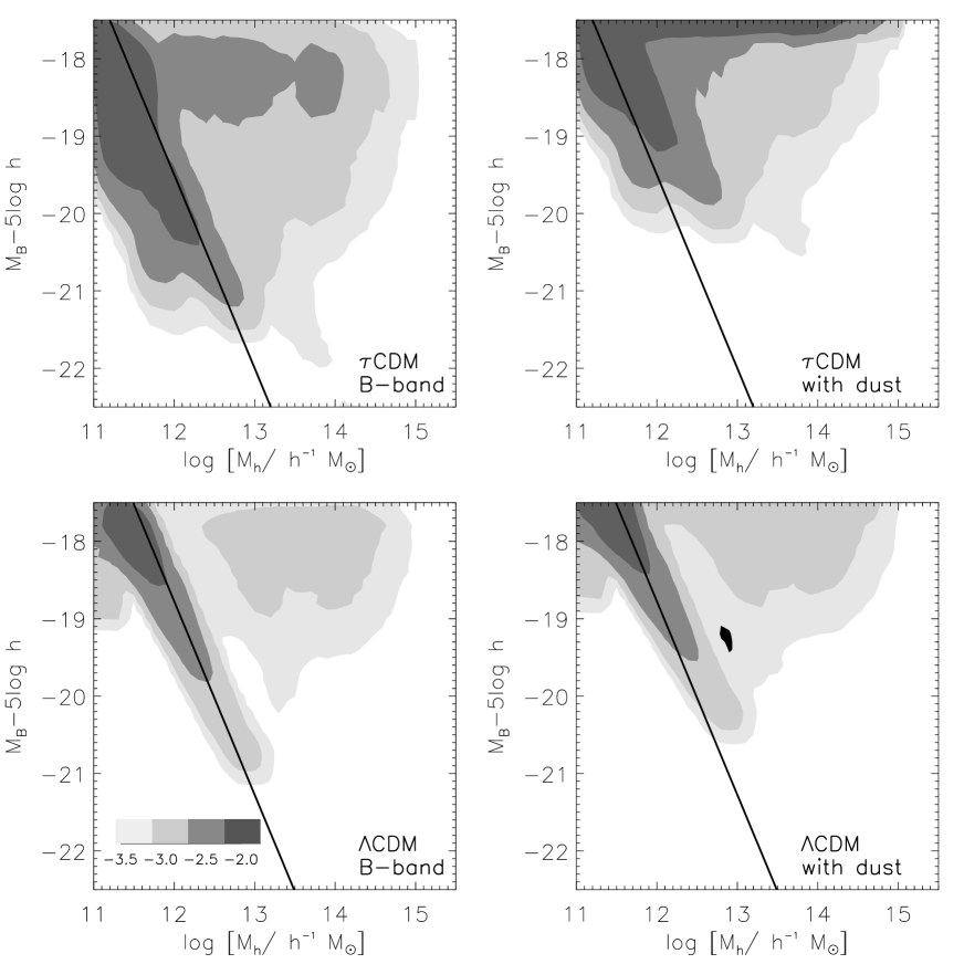
Figure 2: The relationship between galaxy luminosity and the mass of the host halo. The contours represent the joint probability that a galaxy has a given luminosity and dwells in a host halo with a given mass. The grey-scale indicates the $\log_{10}$ of the probability, as shown by the scale bar on the figure. The right panels show the effects of applying a differential correction for dust extinction to the modelled luminosities, in which more luminous galaxies are more extinguished (see text). Top panels show the $\tau$CDM simulations and bottom panels show the $\Lambda$CDM simulations. The diagonal lines indicate constant mass-to-light ratio, with the constant dictated by the observed B-band Tully-Fisher relation.

In general, a single dark-matter halo in our simulations may contain several galaxies with a range of luminosities. The largest collapsed halos in our simulations have virial radii of $1.5-2\mbox{$h^{-1}$ Mpc}$. Therefore, on the smoothing scales that investigate here ($R_{s}\mathrel{\hbox{\hbox to0.0pt{\hbox{\lower 4.0pt\hbox{$\sim$}}\hss}\hbox{$>$}}}4\mbox{$h^{-1}$ Mpc}$), the clustering of galaxies is mainly determined by the clustering of the halos in which they dwell. Figure 2 shows the joint probability function of absolute magnitude and host halo mass for the galaxies in our simulations. The pronounced diagonal “ridge” is populated by galaxies that are the central object in their halo, and illustrates the fairly tight relationship between luminosity and halo mass or circular velocity (i.e. the Tully-Fisher relation) obeyed by these galaxies. This ridge corresponds to a constant halo mass-to-light ratio, where the value of the constant is constrained to agree with the zero-point of the observed Tully-Fisher relation by construction (see Section 3.2). The galaxies that lie far off of the ridge are mainly satellites. Thus we see that galaxies with a given luminosity live in a wide range of environments. The differing appearance of the contours in the two different cosmologies (for example the much broader ridge in the $\tau$CDM simulations) are a direct consequence of the details of the star formation and supernovae feedback recipes, which were chosen to give the best agreement with observations [Kauffmann et al. (1998a)]. Put another way, these two cosmologies have different halo mass functions, so that in order for both to reproduce the observed galaxy luminosity function, the relationship between halos and galaxiesmust be different. The right-hand panels show the results of including dust extinction. We see that this effect can substantially modify the relationship between mass and light in the B-band. We return to this point later.

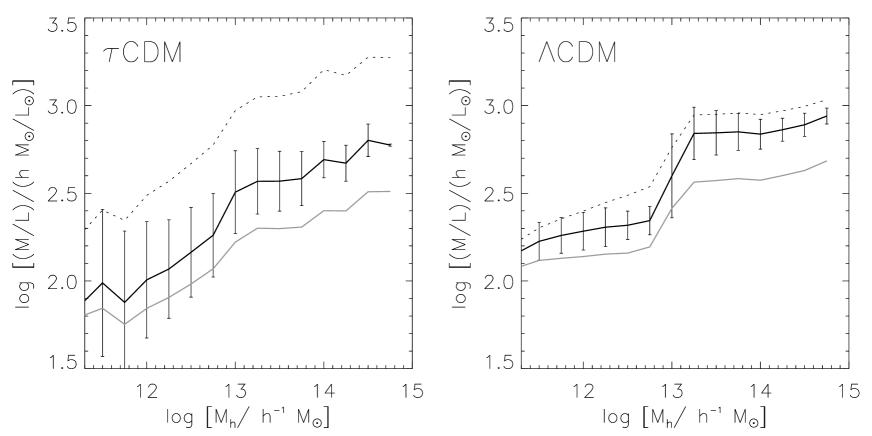
Figure 4: The mass to light ratio of halos in the simulations. The solid black line shows the B-band $M/L$, and error bars show the 1-sigma scatter. The dotted line shows the B-band $M/L$ after a correction for dust extinction has been applied (see text). The grey line shows the I-band $M/L$ (without dust).

Figure 4 shows the mass-to-light ratio of halos in our simulations in the B and I bands. The effective mass-to-light ratio when dust extinction is included is also shown. The mass-to-light ratio varies by more than one order of magnitude from the smallest to largest halos in the simulations, and has a large scatter at a fixed halo mass. The characteristic mass $M_{*}$, defined as the mass that is just becoming non-linear at a particular epoch (more precisely $\sigma(M_{*}(z))=\delta_{c}(z)$), is $M_{*}=2.9\times 10^{12}\mbox{$h^{-1}$ $M_{\odot}$}$ for the $\tau$CDM model and $M_{*}=1.5\times 10^{13}\mbox{$h^{-1}$ $M_{\odot}$}$ for the $\Lambda$CDM model (see figure 6). The exponential turn-over in the halo mass function thus occurs at a mass much larger than that of halos that typically host $L_{*}$ galaxies. Therefore the sharp increase in $M/L$ at $\sim 10^{13}\mbox{$h^{-1}$ $M_{\odot}$}$ is necessary in order to produce a luminosity function with a “knee” at $L_{*}$. This is generally believed to be the result of inefficient cooling in large halos, and in these simulations it is achieved by turning off gas cooling in halos larger than 350 km s^-1(see [Kauffmann et al. (1998a)]). We may also note that the difference between the mean B-band and I-band mass-to-light ratio increases with halo mass, indicating that larger halos tend to host galaxies with redder colours.

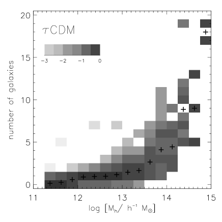
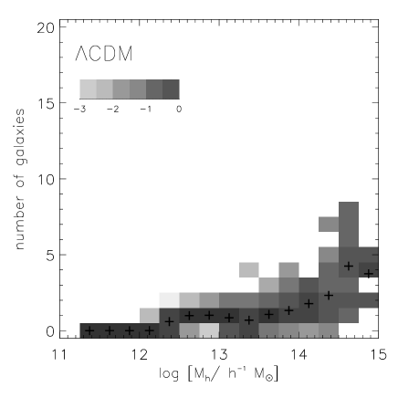
Figure 8: The probability of finding $n$ galaxies per halo, with $M_{B}-5\log h\leq-19.5$, as a function of halo mass, in the $\tau$CDM (top) and $\Lambda$CDM (bottom) simulations. The grey scale indicates the $\log_{10}$ of the probability, according to the scale shown on the figure. The mean is shown by the cross symbols.

The distribution $P(n|M_{h})$ of the number of bright galaxies per halo as a function of halo mass is shown in figure 8. Halos with masses between $10^{12}\mbox{$h^{-1}$ $M_{\odot}$}$ and $10^{13}\mbox{$h^{-1}$ $M_{\odot}$}$ contain one bright galaxy on average, with a relatively small dispersion. Larger mass halos ($\mathrel{\hbox{\hbox to0.0pt{\hbox{\lower 4.0pt\hbox{$\sim$}}\hss}\hbox{$>$}}}5\times 10^{13}\mbox{$h^{-1}$ $M_{\odot}$}$) typically contain more than one galaxy per halo, and the number of galaxies per halo has a larger dispersion; these halos represent groups or clusters of galaxies.

5 Biasing of Halos and Galaxies

In this section we present our main results concerning the biasing relation between the overdensity fields of halos, or galaxies, and that of the underlying dark matter.

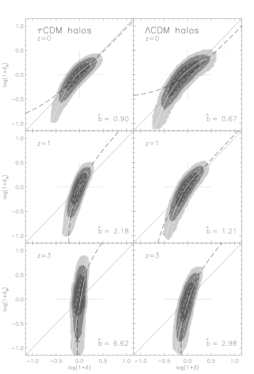
Figure 10: The joint distribution of the overdensity fields of halos ($M\geq 10^{12}\mbox{$h^{-1}$ $M_{\odot}$}$) and mass, both smoothed with a top-hat window of radius $R_{\rm s}=8\mbox{$h^{-1}$ Mpc}$, for $\tau$CDM (left) and $\Lambda$CDM (right), for several redshifts. The contours represent approximately the 50 (dark grey), 80 (medium grey), and 98 (light grey) percentiles. The white lines show the mean conditional biasing function $\langle\delta_{\rm g}|\delta\rangle$ and the $1\sigma$ scatter about it in equal bins of $\log(1+\delta)$. The black long-dashed line shows the linear biasing approximation with $b=\hat{b}$.

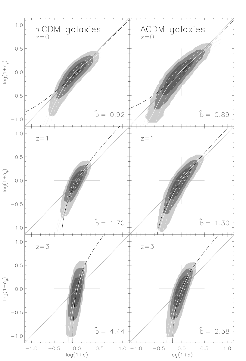
Figure 12: Same as figure 10, for galaxies brighter than $M_{B}-5\log h=-19.5$.

Figure 10 shows the joint distribution $P(\delta_{\rm g},\delta)$ for halos, and figure 12 shows the same for galaxies. All the density fields have been smoothed with a top-hat filter of radius 8 $h^{-1}$ Mpc (hereafter T8). We have selected halos with masses larger than $1.0\times 10^{12}\mbox{$h^{-1}$ $M_{\odot}$}$, and galaxies with $M_{B}-5\log h\leq-19.5$, at several redshifts as indicated on the figures. The conditional mean and standard deviation functions are shown, corresponding to $b(\delta)$ and $\sigma_{\rm b}(\delta)$ of Eqn. 3 and 7. Shown for reference is also the linear biasing approximation $\delta_{\rm g}=b\delta$, with $b=\hat{b}$. A log-log density plot is used in order to stress the behavior in the regions of under-density. Note that in this specific presentation, linear biasing appears as a curved line.

The results for halos and galaxies are qualitatively similar. This is somewhat surprising given the rather complex relationship between the two that we saw in the previous section. However, recall from figure 8 that on average there is approximately one galaxy brighter than $-19.5+5\log h$ per $\sim 10^{12}\mbox{$h^{-1}$ $M_{\odot}$}$ halo. These halos are much more numerous than the larger mass halos that host larger numbers of galaxies, so they tend to dominate the appearance of a number-weighted joint probability such as the quantity represented in these figures. We also note that the contours for the two cosmological models differ in their details but overall they appear qualitatively similar.

The favored environment for halo/galaxy formation, namely, the peak in the halo/galaxy overdensity distribution, occurs in regions where the matter density is close to its mean value ($1+\delta=1$). In the vicinity of $1+\delta\sim 1$, the overdensity of halos/galaxies follows that of the underlying matter, $b(\delta)\simeq 1$. But, in general, the linear biasing approximation is not an accurate description of the mean biasing relation.

The mean biasing function shows a robust characteristic behavior in the under-dense regions ($1+\delta<1$); the local slope of $b(\delta)$ is steeper than the global slope $\hat{b}$, and is larger than unity even when $\hat{b}<1$. This leads to voids empty of galaxies below some finite matter underdensity ($1+\delta>0$); namely, the galaxy-formation efficiency drops to zero below a certain mass-density threshold. We can say that the galaxies in the voids are always “positively biased”, in the sense that locally $\hat{b}>1$, while they can be either biased or “anti-biased” ($\hat{b}<1$) in the high-density regions.

In the over-dense regions ($1+\delta>1$), the behavior changes with redshift. At $z=0$, the local slope of $b(\delta)$ is smaller than unity, driving $\hat{b}$ to below unity. At higher redshifts the local slope becomes larger, driving $\hat{b}$ to values as large as 3 to 7 by $z=3$. The redshift dependence of the biasing relation is striking; we return to it in 5.4.

The stochasticity in the biasing scheme is evident from the spread in $\delta_{\rm g}$ at fixed $\delta$. We will discuss it further in the next section.

5.1 Mass and Luminosity Dependence

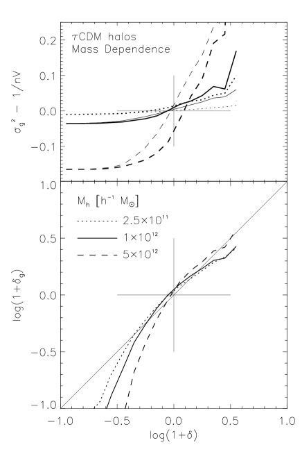
Figure 14: Mass dependence of the mean and scatter of the conditional biasing relation for halos, for $\tau$CDM at $z=0$. The bottom panel shows the mean conditional biasing relation for halos in our simulations, selected with different mass thresholds. The top panel shows the variance of the conditional biasing relation, minus the mean expected variance due to shot noise. Bold lines indicate the simulation results and light lines indicate the “conditional Poisson” model discussed in the text.

In this section we investigate the dependence of biasing on halo mass and galaxy luminosity, for a fixed smoothing window (T8) and at the present epoch ($z=0$). Figure 14 (bottom) shows the mean biasing function for halos selected with different mass thresholds, in the $\tau$CDM simulation. We see that massive halos are more biased; the curves all cross at $\delta\simeq 0$, massive halos have higher overdensities than smaller mass halos in regions with $\delta>0$, and smaller mass halos have higher overdensities where $\delta<0$.

The top panel shows the variance of the conditional biasing distribution $\langle\epsilon^{2}|\delta\rangle$ minus the mean shot noise correction $1/(\bar{n}V_{s})$, where $\bar{n}=N/V_{\rm BOX}$ is the average number density of halos/galaxies above the given threshold in the simulation, and $V_{s}$ is the volume of the smoothing window. The conditional Poisson model discussed in Section 2.2.3 is shown for comparison. In regions of lower than average overdensity, the scatter is generally smaller than the mean shot noise, and in overdense regions it is larger.

This can be understood by referring to the expression for the variance of counts in cells [Peebles (1980)]:

$$\mu_{2}\equiv\langle(N-nV)^{2}\rangle=nV+n^{2}\int_{V}dV_{1}dV_{2}.\xi_{12}$$ (17)

The variance of the conditional biasing distribution is then $\mu_{2}/(nV)^{2}$. This reduces to the usual shot noise value $1/\sqrt{nV}$ in the absence of correlations ($\xi=0$), but it leads to a scatter larger than the mean shot noise when the integral over $\xi$ is positive, and smaller than the mean shot noise when it is negative. In underdense regions ($\delta<0$), halos are anti-correlated ($\xi<0$) and the volume-averaged correlation function, $\bar{\xi}$, is negative. In overdense regions ($\delta>0$), halos are positively correlated and $\bar{\xi}$ is positive.

The corresponding results for the $\Lambda$CDM model are extremely similar (and are therefore not shown) because the mass dependence enters only through the shape of the power spectrum, which is similar by design for the $\tau$CDM and $\Lambda$CDM simulations.

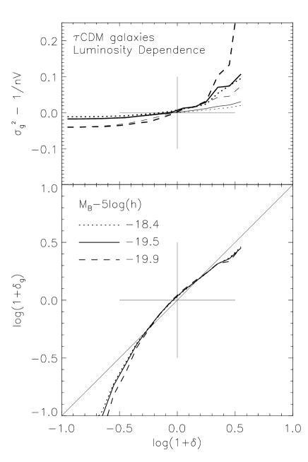
Figure 16: Same as figure 14, for galaxies selected with different B-band absolute magnitude thresholds.

Figure 16 summarizes the mean and scatter of the conditional biasing relation for galaxies with different luminosity thresholds. Two notable features are evident. First, we see no significant change in the biasing relation for galaxies with absolute-magnitude thresholds in the range $-18.4+5\log h$ (well below $L_{*}$) to $-19.9+5\log h$ (above $L_{*}$). We return to this point in a moment, when we discuss figure 22. Second, the scatter compared to the average shot noise is comparable to the corresponding quantity for halos. On the face of it, one might think that the complex physics of gas cooling, star formation, merging, supernovae feedback, etc, even as simply modelled in our simulations, would lead to a larger scatter. However, on the other hand, the nature of the physics associated with these processes might actually lead to a stronger correlation of luminosity with the local matter density than that shown by the halos. For example, gas can only cool and form stars in regions with sufficiently high density, the star formation efficiency is assumed to be proportional to the density, supernovae feedback is less efficient in halos with deep potential wells (i.e. high density), and starbursts occur preferentially in high density regions. While these lines of argument appear plausible, more detailed investigation of the physical source of scatter in the biasing relation that we obtain both for galaxies and halos is clearly in order.

The three characteristic parameters of the biasing scheme (see Section 2.1), measuring mean biasing, nonlinearity, and stochasticity, are shown in figure 18 as a function of halo-mass threshold or galaxy luminosity threshold. The mean biasing is characterized by $\hat{b}$, and also shown are $b_{\rm var}$ and $b_{\xi}$. The fact that $b_{\rm var}$ tends to be systematically larger is due to the presence of nonlinearity and stochasticity. The nonlinearity, as measured by $\tilde{b}/\hat{b}$, is less than 10 percent for halos and is nearly constant over the mass range. The nonlinearity is even smaller for galaxies, and shows a trend with galaxy luminosity. The stochasticity, $\sigma_{\rm b}/\hat{b}$, shows a modest trend, increasing for higher mass halos or brighter galaxies. As remarked before, the stochasticity is actually larger for halos than for galaxies. The linear correlation coefficient $r=\hat{b}/b_{\rm var}$, which, like $b_{\rm var}$, mixes nonlinear and stochastic effects, is roughly constant over these ranges of mass or luminosity and has a value $r\simeq 0.9$.

We further examine the clustering of halos of different masses compared to the dark matter in figure 20, which shows the auto-correlation functions of halos and dark matter in the $\tau$CDM simulations. More massive halos show correlations of higher amplitude and therefore more positive biasing. The turn-over of the halo correlation functions at small radii is caused by exclusion effects due to the finite spatial extent of the halos. When using conventional halo finders based on friends-of-friends or spherical over-density, halos that lie too close together are “merged” into a single halo. The spatial scale at which this effect becomes important depends on the mass of the halo, according to the relation between virial radius and mass ($M_{\rm vir}\propto r^{3}_{\rm vir}$). Thus on small scales, one expects anti-correlations due to this exclusion effect to lead to negative $\bar{\xi}$ in regions of high halo density, and thus to a reduction in the scatter, but this effect is negligible for the smoothing scales considered here ($R_{\rm s}\mathrel{\hbox{\hbox to0.0pt{\hbox{\lower 4.0pt\hbox{$\sim$}}\hss}\hbox{$>$}}}4\mbox{$h^{-1}$ Mpc}$). Note that the fact that the observed galaxy correlation function is a nearly perfect unbroken power-law on sub-Mpc scales indicates that there must be a significant contribution from galaxy pairs that dwell within a common halo.

The correlation function of galaxies with different luminosity thresholds is shown in figure 22. As noted by ?), the clustering amplitude of the galaxies in the simulations is nearly independent of the luminosity threshold, in contrast to the findings of ?), who observed pronounced luminosity-dependent bias in the SSRS2 redshift survey. They found that brighter galaxies are more strongly clustered than fainter galaxies, and thus have a longer correlation length $r_{0}$ as shown on the figure.

Our result is not surprising given the weak mass dependence of the biasing of galaxy-mass halos (figure 18). However, this introduces an apparent problem when compared to observations. The difference between the faintest and brightest magnitude thresholds for the observed galaxy samples analyzed by ?) is about 1.5 magnitudes. This corresponds to a factor of four in mass if the mass-to-light ratio is constant and its value is dictated by the observed Tully-Fisher relation. On the other hand, we saw from figure 18 that there is only a $\sim 10\%$ increase in the mean biasing as a function of halo mass over this range, and even this weak mass dependence is diluted by the presence of low-luminosity satellite galaxies in large-mass halos (see figure 2), yielding no luminosity dependence in our simulated galaxy biasing.

A clue for a resolution of this problem may come from the fact that the mass dependence of halo biasing becomes much stronger in the regime where $M>M_{*}$ (figure 18). If we increase the mass-to-light ratio, pushing the bright galaxies into larger mass halos, we would obtain stronger luminosity dependence, as was in fact found by ?) when they effectively normalized their models with a higher mass-to-light ratio. Unfortunately, this would lead to an apparent contradiction with the observed Tully-Fisher relation.

A more promising way to achieve the desired effect is by inclusion of dust in our considerations. We note that the observed Tully-Fisher relation has been corrected for dust extinction using observationally determined inclinations for each galaxy. These corrections can be quite large in the B-band, where most of the samples used to study galaxy clustering are selected. Moreover, there is evidence that more luminous galaxies suffer larger extinctions [Tully et al. (1999), Wang & Heckman (1996)]. Studies of galaxy clustering do not include corrections for dust extinction because inclination estimates are generally not available. ?) showed that including dust extinction can significantly modify the galaxy-galaxy correlation function found in these simulations.

The $\tau$CDM model suffered from an excess of bright galaxies compared to the observed B-band luminosity function when dust extinction was neglected. ?) found that including dust extinction using the empirical recipe of ?) led to an improved luminosity function, but still with an excess, especially on the bright end. We now tune the parameters of the WH recipe in order to obtain the best possible fit to the observed luminosity function. For the $\tau$CDM model, we find that using $\beta=0.2$ and setting $\tau^{*}_{B}=2.0$ in eqn. 16 gives the best results. For the $\Lambda$CDM model, the luminosity function already has a small deficit of galaxies compared to observations even without any dust correction. Despite this, we show the results of applying a dust correction to the $\Lambda$CDM models using the fiducial values of the WH parameters (as in [Kauffmann et al. (1998a)]).

The inclusion of dust extinction changes the effective mass-to-light ratio of the halos in the simulations (see figure 2), in the desired sense: galaxies of a given observed luminosity now dwell in larger mass halos. We see in the right-hand panels of figure 22 that this leads to a luminosity dependence that is qualitatively similar to the observed dependence, especially in the $\tau$CDM case (unfortunately, the number of bright galaxies in our simulation box also becomes quite small, and the correlation function becomes rather noisy, but the trend is clear). Note also that although the inclusion of dust increases the correlation amplitude of the galaxies in the $\tau$CDM model, bringing the results into better agreement with the observed galaxy correlation function, the clustering amplitude for bright galaxies is still not as high as the SSRS2 observations. Conversely, with no dust correction, the clustering amplitude of galaxies for the $\Lambda$CDM model is already comparable to the observational results, and inclusion of dust hardly makes a difference. It may be that a cosmology with an intermediate value of $\Omega_{0}\simeq 0.5$ will give the best overall results when realistic extinction due to dust is included. However, a much larger correction seems to be required in order to match the correlation function of very bright galaxies as provided by these observations. These results highlight the importance of obtaining large redshift surveys selected in near IR bands in order to reduce the sensitivity to dust extinction.

5.2 Type Dependence

We study the type dependence of biasing with T8 smoothing, for galaxies brighter than $M_{B}-5\log h=-18.4$, at $z=0$. Here, instead of quantifying the bias of galaxies with respect to mass as in the previous section, we show the biasing of different types of galaxies relative to the overall galaxy population. This relative bias is of particular practical interest because it can be compared directly with the results of observations.

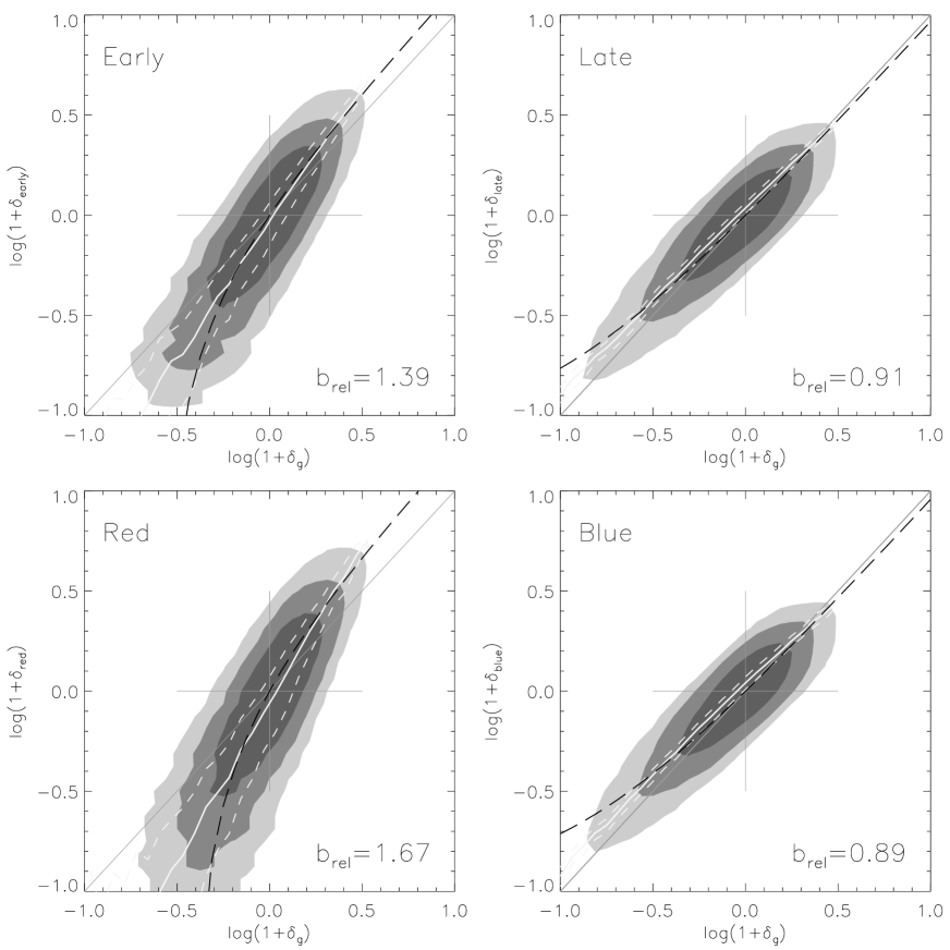
Figure 24: The joint distribution of the overdensity fields of type-selected galaxies and all galaxies, both with $M_{B}-5\log h\leq-18.4$ and smoothed with a top-hat window of radius $R_{\rm s}=8\mbox{$h^{-1}$ Mpc}$, for the $\tau$CDM simulations. The top panels represent galaxies selected by morphology (“early” corresponds roughly to E–S0, “late” to S–Irr Hubble types), and the bottom panels represent galaxies selected according to B-V colour. The contours represent approximately the 50 (dark grey), 80 (medium grey), and 98 (light grey) percentiles. The white lines show the mean conditional biasing function $\langle\delta_{\rm early/late}|\delta_{\rm g}\rangle$ and the $1\sigma$ scatter about it in equal bins of $\log\delta_{\rm g}$. The black long-dashed line shows the linear biasing approximation with $b=\hat{b}_{\rm rel}$.

We can classify different types of galaxies in our simulations in several ways. For example, we identify “early” and “late” types according to the bulge-to-total luminosity ratio; galaxies of $L_{\rm bulge}/L_{\rm tot}>0.4$ are identified with early type galaxies (Hubble type E–S0), and the rest with late types (S–Irr), as in ?). Similarly, we can divide the galaxies in terms of colour. Here, we classify galaxies with $B-V>0.8$ as “red” and the remainder as “blue”. Figure 24 (top) shows the joint density distribution for galaxies of early and late types relative to the galaxy population as a whole at the same magnitude limit. Early type galaxies are biased ($\hat{b}>1$) compared to the overall population, wheras late type galaxies are slightly anti-biased ($\hat{b}<1$) We obtain comparable results, with stronger bias and anti-bias, when galaxies are divided in terms of their colors, as shown in the bottom panels. The results shown are for the $\tau$CDM simulation, and are similar for the $\Lambda$CDM simulation.

Once again, we can understand this result in terms of the masses of the dark matter halos in which these different types of galaxies are found. Figure 26 shows the distributions of host halo masses for early and late type galaxies and red and blue galaxies. Although each type occupies a broad range of halo masses, the mean halo mass occupied by early/red types is significantly larger than that occupied by late/blue types. Several physical effects included in the semi-analytic modelling may contribute to this result. Larger mass halos are more likely to have suffered a recent major merger, which is assumed to destroy the disk and create a bulge. In addition, gas cooling ceases in large mass halos, cutting off the supply of new gas and subsequently the star formation. Therefore the galaxies in these halos redden, are not able to form new disks and so remain bulge-dominated. Note that the separation between the distributions of red and blue galaxies is larger than the separation between early and late types (figure 26), explaining why the relative biasing is stronger for the former (figure 24).

The mean relative biasing parameters found in the simulations are summarized in Table 4. These parameters are the equivalent of $\hat{b}$ and $b_{\rm var}$ as defined in Section 2.1, where the matter field $\delta$ is replaced with the field of late/blue type galaxies and $\delta_{\rm g}$ is replaced with the field of early/red type galaxies. The difference between $\hat{b}^{\rm rel}$ and $b_{\rm var}^{\rm rel}$ again indicates the presence of nonlinearity and stochasticity in the relative biasing relation, and is also reflected in the relative linear covariance parameter $r^{\rm rel}$.

Table 4: Relative bias of early to late and red to blue galaxies in the simulations on a scale of 8 $h^{-1}$ kpc. For each parameter, the first value is for $\tau$CDM and the second is for $\Lambda$CDM.

type	$\hat{b}^{\rm rel}$		$b_{\rm var}^{\rm rel}$		$r^{\rm rel}$
early/late	1.4	1.1	1.5	1.3	0.93	0.87
red/blue	1.6	1.6	1.8	1.8	0.87	0.87

Observationally, the stronger clustering of early type galaxies is well known [Dressler (1980), Hermit et al. (1996), Willmer et al. (1998), Tegmark & Bromley (1998)]. In order to compare with theoretical predictions, care must be taken to account properly for the transformation from redshift space to real space, as early and late type galaxies are known to be affected differently by redshift distortions. In real space, ?) find $b_{\rm early}/b_{\rm late}=1.18\pm 0.15$, ?) find $b_{\rm early}/b_{\rm late}=1.33$ and ?) find $b_{\rm early}/b_{\rm late}=1.68$. Not surprisingly, the range of observational values seems to depend on the importance of clusters in the sample, with higher values obtained in samples that include many rich clusters. The quoted observational statistics correspond to $b_{\rm var}$. The values we obtain (1.3-1.5) are in reasonable agreement with the observational values.

It is also fairly well established that red galaxies are generally more clustered than the blue population [Landy et al. (1996), Tucker et al. (1997)], but a quantitative comparison is more difficult, because most of the values in the literature are obtained from the angular or redshift space correlation functions, and a variety of colour bands are used. ?) quote a relative variance bias in real space $b_{\rm red}/b_{\rm blue}=1.40\pm 0.33$ at $8\mbox{$h^{-1}$ Mpc}$, and suggest that there is evidence for scale dependence in the relative bias. However, they used a colour threshold of $B-R=1.3$ so it is not directly comparable with our results.

In principle, the type dependence could be further studied as a function of redshift, scale, luminosity, or environment. The samples currently available from both simulations and observations are too small to obtain proper statistics after this sort of subdivision, but this may be a powerful discriminatory tool for galaxy formation models once larger simulations and larger redshift surveys are available. Another promising approach would be to categorize galaxies using automatic spectral classification methods such as Principal Component Analysis [Connolly et al. (1995), Folkes et al. (1996)] and study the corresponding relative bias. An example of a comparison of this sort appears in ?).

5.3 Scale Dependence

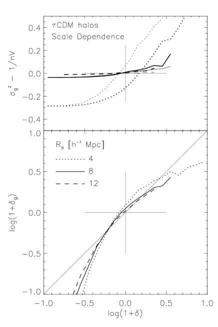
Figure 28: Scale dependence of the mean and scatter of the conditional biasing relation for halos ($M\geq 10^{12}\mbox{$h^{-1}$ $M_{\odot}$}$), for $\tau$CDM at $z=0$. The quantities shown are as in figure 14.

Figure 28 and 30 show the scale dependence of biasing for a fixed halo mass threshold ($M\geq 10^{12}\mbox{$h^{-1}$ $M_{\odot}$}$) or galaxy luminosity ($M_{B}-5\log h\leq-19.5$) at the present epoch ($z=0$). The results shown are for top-hat smoothings of 4, 8 and 12$h^{-1}$ Mpc. This figure shows the mean and scatter of the conditional biasing relation for halos in the $\tau$CDM simulation (again, the results of the $\Lambda$CDM simulation are nearly identical and are not shown). The scale dependence of the mean biasing is weak over this range, while the scatter shows an expected scale dependence. Once again, the results for galaxies are similar to the results for halos. This suggests that, at least in our simulations, the scale dependence (or lack thereof) of biasing of bright galaxies is mainly determined by the gravitational physics of halo formation.

Figure 32 presents the scale dependence of the biasing parameters. Here we see that the mean biasing actually increases slightly with smoothing scale for both halos and galaxies. As expected, the non-linearity and stochasticity both decrease with increasing smoothing scale, such that the biasing relation converges towards linear deterministic biasing for large smoothing scales.

5.4 Redshift Dependence

We now return to the redshift evolution of biasing, which is the most striking feature in figure 10 and 12, and is of particular interest given the recent observational developments at high redshift. We use a fixed halo-mass threshold ($M\geq 10^{12}\mbox{$h^{-1}$ $M_{\odot}$}$) or luminosity threshold ($M_{B}-5\log h\leq-19.5$) and smoothing scale (T8). We already noted that the shape of the biasing relation changes noticably, and in particular the slope $\hat{b}$ increases dramatically with redshift. The rapid evolution towards higher bias at high redshift has been noted in several recent works [Bagla (1998), Wechsler et al. (1998), Colín et al. (1998), Katz et al. (1998), Blanton et al. (1999)]. Here we discuss several other interesting properties of the redshift evolution of biasing of both halos and galaxies.

The $\tau$CDM and $\Lambda$CDM models, which showed very similar mass and scale dependences at $z=0$, show quite different redshift evolution. The evolution is more pronounced in the $\Omega_{0}=1$ $\tau$CDM model than in the low-$\Omega_{0}$ $\Lambda$CDM model, as expected. This is because the mass and scale dependence at fixed redshift are determined mainly by the shape of the power spectrum, which is deliberately similar for these two models, while the redshift evolution depends on the growth rate of clustering, which is quite different in these two models.

In addition, we can see in figure 10 and 12 that the evolution of the biasing relation for galaxies is weaker than that for halos. This is because of the redshift dependence of the efficiency of star formation and hence of the relationship between halo mass and galaxy luminosity. Halos are typically denser at high redshift, and in these models we have effectively assumed that the star formation rate is proportional to the average halo density (see figure 8 and 9 of ?) and Eqn. 14 of this paper). Therefore, when we select galaxies with a fixed luminosity threshold, at high redshift we include galaxies residing in smaller mass halos (and thus of lower biasing). Note that this effect also reduces the difference in the evolution of biasing within the two cosmological models, i.e., the additional physics associated with star formation conspires to make the redshift evolution of biasing less discriminatory to cosmology.

Figure 34 summarizes the redshift evolution of the mean bias, nonlinearity, and stochasticity parameters. Note the increasing difference between the mean biasing statistics, $\hat{b}$, $b_{\rm var}$ and $b_{\xi}$, with increasing redshift, for the $\tau$CDM model; $\hat{b}$ differs from $b_{\xi}$ by a factor of two at $z=3$. This difference reflects the increase in stochasticity and non-linearity with redshift in the $\tau$CDM model, as seen in the lower panels of the figure. The increase in stochasticity in this model is dominated by the increase in shot noise due to the decrease in number density of halos/galaxies between $z=1$ and $3$. The difference in $b_{\xi}$ and $b_{\rm var}$ is due to the stronger scale dependence at $z=3$ ($b_{\xi}$ reflects the biasing at a fixed scale, whereas $b_{\rm var}$ is an average over different scales). In the $\Lambda$CDM simulations, the non-linearity and stochasticity instead decrease with redshift, and therefore $\hat{b}$, $b_{\rm var}$ and $b_{\xi}$ agree within 30 percent at $z=3$. Thus, the evolution of the biasing parameters is characterized in the two models by a minimum in the nonlinearity and stochasticity, which occurs at $z\sim 1$ in the $\tau$CDM cosmology and $z\sim 3$ in the $\Lambda$CDM cosmology.

Some insight into the origin of this minimum may be gained by examining the time evolution of the correlation functions of dark matter, halos, and galaxies from $z=3$ to $z=0$, shown in figure 36. The clustering amplitude of the dark matter increases monotonically as time progresses. However, halos of a fixed physical mass correspond to rarer peaks in the density field at higher redshift, so the clustering amplitude of these objects decreases monotonically as time moves forward. The changing mass scale corresponding to galaxies of a fixed B-band luminosity discussed above leads to a rather different behaviour for the magnitude-limited galaxies. In both models, the clustering amplitude decreases as we move backwards in time from $z=0$ to $z=1$. It starts increasing at a redshift of about $z=1$ for $\tau$CDM and $z=3$ for $\Lambda$CDM. This effect is discussed in much more detail in ?), who found that the magnitude of this “dip” in the clustering amplitude or correlation length depends on the way in which galaxies are selected as well as on the cosmology. In both models investigated, the redshift at which the the correlation amplitude begins to rise corresponds approximately with the minimum in the non-linearity and stochasticity of the biasing relation noted above. This correspondance is intriguing but its significance is not immediately obvious.

6 Comparison with Analytic Models of Biasing

Analytic models of biasing provide an important counterpart to $N$-body simulations, which have limited resolution and volume. In this section we evaluate several biasing models by comparing them with the results of our simulations, focussing especially on the redshift dependence. Numerous recent papers [Matattese et al. (1997), Moscardini et al. (1998), Adelberger et al. (1998), Coles et al. (1998), Mo et al. (1998), Magliocchetti et al. (1999)] have made use of versions of these analytic models to make predictions about galaxy clustering at high redshift and to interpret high-redshift observations.

We first investigate the Mo & White model, summarized in Section 2.2.2. In their original paper, ?) showed that their model agreed well with the results of simulations with scale-free power spectra. It is useful to investigate their model in the context of a more realistic power spectrum, and to show results in terms of the physical mass scales and redshifts that we expect to correspond to observable galaxies. For technical convenience, we display the biasing relation as a function of mass threshold, while MW originally provided predictions for halos of a specific mass. To compute the MW prediction for all masses above a threshold, we simply perform a weighted average over the original expression (MW eqn. 19), using the Press-Schechter formula for the number density of halos of a given mass [Press & Schechter (1974)].

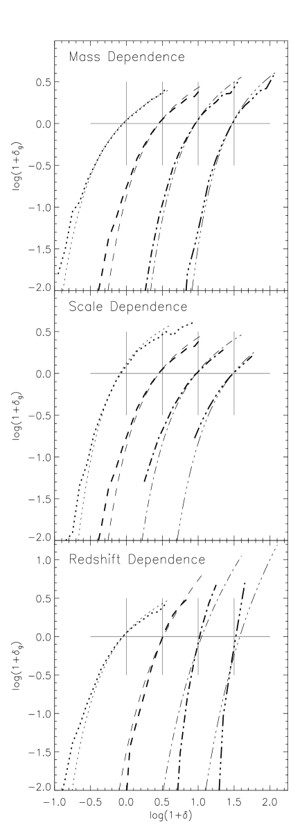
Figure 38: Comparison of the predictions of the MW model (light lines) with the simulation results (bold lines) for the mean biasing relation. The curves in each panel have been offset by 0.5 dex for clarity. The top panel shows the results for different mass thresholds ($\log[M/(\mbox{$h^{-1}$ $M_{\odot}$})]=11.4,12.0,12.4,12.7$ from left to right), the middle panel shows different smoothing scales ($R_{s}=4,8,12,16\mbox{$h^{-1}$ Mpc}$ from left to right) and the bottom panel shows different redshifts ($z=0$, 1, 2, 3 from left to right).

Figure 38 shows the comparison of the MW predictions for the mean biasing relation with the simulation results ($\tau$CDM) for halos at different mass thresholds, smoothing scales, and redshifts. Apparently the MW model does well at reproducing the changing shape of the biasing relation with mass, scale, and to a lesser extent, redshift. At $z=0$, the MW model tends to slightly underpredict the halo overdensity in regions of very low matter overdensity. At larger redshifts, the MW model fails to follow the rapid growth of the slope $\hat{b}$ with redshift. The progressively larger deviation of the MW predictions from the simulation results with increasing redshift is probably the result of inaccuracies in the underlying Press-Schechter and extended Press-Schechter approximations, which are known to have a similar redshift dependence [Somerville et al. (1998)]. However, the MW model does correctly predict the qualitative features of the evolution, including both the change in shape and the progression towards higher biasing.

As we mentioned in Section 2.2.2, when the overdensity within the smoothing window is low compared to the critical overdensity for collapse at a particular epoch, the MW model reduces to a very simple expression for the linear bias factor b(M, z) as a function of halo mass and redshift (MW eqn. 20, our eqn. 13). Figure 40 shows the mass dependence of the halo biasing parameter $b_{\rm var}$ at several redshifts for the simplified MW model and the $\tau$CDM simulations. Even this simple expression agrees remarkably well with the mass and redshift dependence of biasing of halos in our simulations. The mass range of halos that can be usefully studied in our simulations is limited on the low mass end by our resolution ($M_{\rm res}=2.0\times 10^{11}M_{\odot}$) and on the high mass end by shot noise. In the figure, we show the simulation results both with and without a standard Poisson correction for shot noise. Particularly for high mass halos, the sampling is far from Poisson and the shot noise correction is likely to be inaccurate. Another interesting thing to note is that the mass dependence of biasing over scales comparable to the size of galactic halos ($\sim 10^{11}-10^{12}\mbox{$h^{-1}$ $M_{\odot}$}$) is much stronger at high redshift than at $z=0$. This is because of the dramatic decrease of the non-linear clustering mass $M_{*}$ with redshift (see figure 6).

The time evolution of $b_{\rm var}$ for halos ($M>10^{12}\mbox{$h^{-1}$ $M_{\odot}$}$) and galaxies ($M_{B}-5\log h\leq-19.5$) is compared with the predictions of the models in figure 42. One can clearly see the slower evolution of galaxies versus halos in the simulations, discussed in Section 5.4. We show the MW model (eqn. 13) for the corresponding mass threshold. The MW model gives a good qualitative description of the evolution of halo biasing, as noted before.

There is no mass threshold that gives a good description of the evolution of the galaxy biasing, because of the differing merger timescales of galaxies and halos, and because of the effects mentioned earlier concerning the changing mass-to-light connection as a function of redshift.

We also show the galaxy-conserving (GC) model [Fry (1996), Tegmark & Peebles (1998)] described in Section 2.2.1. We start at high redshift ($z=3$ or $z=1$) with the values of $b_{\rm var}$ and the linear correlation coefficient $r$ as measured from the simulation galaxies or halos, and propagate the bias to $z=0$ using eqn. 11. The evolution predicted by the GC models is much weaker than that predicted by the MW models and observed in the simulations. This clearly suggests that merging, which is not included in the GC model, is an important process in the evolution of clustering over this redshift range, even in a low-$\Omega$ Universe. We might expect that merging would be less important for galaxies than halos, and indeed the weak evolution according to the GC model is slightly closer to the biasing evolution for the galaxy population, but it still significantly underpredicts the rate of evolution.

7 Summary and Conclusions

We have performed a study of biasing of dark-matter halos and galaxies in cosmological simulations of $\Lambda$CDM ($\Omega=0.3$) and $\tau$CDM ($\Omega=1$), explicitly treating and quantifying the mean biasing as well as non-linearity and stochasticity in the biasing relation. We conclude that the CDM-based hierarchical structure formation scenario predicts that biasing has a moderate degree of nonlinearity and stochasticity, and it depends on mass, type, scale and especially redshift.

The mean biasing function is always of the following characteristic shape. In the underdense regime ($-1<\delta<0$), $b(\delta)$ vanishes near $\delta\lower 2.15277pt\hbox{$\;\buildrel>\over{\sim}\;$}-1$, then rises sharply towards $\delta_{\rm g}\simeq\delta=0$ with a slope steeper than unity. In the overdense regime ($\delta>0$), the behavior is fairly linear, and the effective slope of $b(\delta)$ is either larger or smaller than unity, representing biasing or anti-biasing. The nonlinearity at $8\mbox{$h^{-1}$ Mpc}$ is at the level of a few to $\sim$10 percent. The stochasticity is typically at the level of a few tens of percent.

For halos, we find that the mean biasing increases gradually with mass, as does the stochasticity (to a large extent due to an increasing shot noise contribution), while the non-linearity is nearly the same for all masses. At $z=0$, the biasing relation for galaxies in our simulations is similar to that for $\mathrel{\hbox{\hbox to0.0pt{\hbox{\lower 4.0pt\hbox{$\sim$}}\hss}\hbox{$>$}}}10^{12}\mbox{$h^{-1}$ $M_{\odot}$}$ halos. This reflects the fact that our halos of $10^{12}\mbox{$h^{-1}$ $M_{\odot}$}$ contain on average one bright galaxy per halo, but is still somewhat surprising given that the halos do contain different numbers of galaxies with various luminosities. We find that the biasing is nearly independent of the luminosity of the galaxies selected, in contradiction with some observational results, but in keeping with our finding of weak mass dependence of halo biasing over the mass scales typical of galaxy-sized halos at $z=0$.

This apparent contradiction may be resolved by considering dust extinction. We show that including the effects of dust effectively increases the mass-to-light ratio, so that $L>L_{*}$ galaxies are found in larger mass halos where the biasing dependence on mass is more pronounced. This leads to a luminosity dependent biasing that is qualitatively similar to that observed, although neither of the cosmological models considered here fully succeed in simultaneously reproducing the amplitude of the observed correlation function and the detailed luminosity dependence of galaxy clustering. We suspect that a cosmology with an intermediate value of $\Omega_{0}\sim 0.5$ might give better results. However, the observational results are still somewhat controversial, and the modelling of dust extinction is highly uncertain. Since this appears to have the potential to be a rather powerful constraint, the relative biasing of galaxies of different luminosities should be measured more accurately using larger samples. Ideally, this should be investigated using a K-band selected sample which will decrease the uncertainties connected with dust extinction.

We find that galaxy biasing depends fairly strongly on morphological type and color, with early type and red galaxies being respectively about 1.3 to 1.8 times more biased than late type or blue galaxies. These results are in good agreement with current observational estimates. More detailed studies of relative biasing will be an important application of forthcoming large redshift surveys such as 2dF, SDSS, and 2MASS.

Over the range of smoothing scales from $4$ to $16\mbox{$h^{-1}$ Mpc}$, the mean biasing increases weakly with smoothing scale, similarly for halos and galaxies.

The non-linearity and stochasticity decrease with increasing smoothing scale, so that the linear deterministic biasing approximation is approached for very large smoothing scales, as expected. On scales larger than a few Mpc, the clustering of bright galaxies in our simulations is fairly robust to differing assumptions about the details of galaxy formation. On smaller scales, halos become strongly anti-correlated because of exclusion effects. This implies that in order to reproduce the observed unbroken powerlaw correlation function of galaxies on these scales, there must be a significant number of galaxy pairs that cohabit the same halo. The biasing of our simulated galaxies on these scales is highly sensitive to the details of the astrophysical recipes, e.g., supernovae feedback, dust extinction, etc.

The mean biasing of halos of a fixed mass and smoothing scale increases dramatically with redshift, by a factor of 5-10 for $\tau$CDM and a factor of $\sim 3$ for $\Lambda$CDM from $z=0$ to $z=3$. In both models, the nonlinearity of the biasing relation evolves with redshift, decreasing to a minimum value very close to 1.0 (pure linear bias) at $z\sim 1$ for $\tau$CDM and $z\sim 3$ for $\Lambda$CDM, then increasing again at higher redshift. The redshift dependence of biasing of galaxies with a fixed luminosity threshold differs significantly from that of halos with a fixed mass threshold. This is because, due to our standard star-formation recipe, galaxies of a given luminosity are hosted at higher redshift by halos of smaller masses and thus of weaker biasing.

We have compared the results of the numerical simulations with analytic models for biasing. The MW model provides a good description of the changing shape of the biasing relation for halos as a function of mass threshold, smoothing scale, and more qualitatively, redshift. Even the simplified linear version of the MW model (Eqn. 13) provides a fairly accurate description of the mass dependence of mean halo biasing and the redshift evolution of halos of a fixed mass. The evolution of galaxy biasing may differ substantially depending on the efficiency of star formation and how it varies with redshift. Galaxy-conserving models (e.g. [Fry (1996)]; ?)) substantially underpredict the evolution rate of halo and galaxy biasing at all epochs, strongly suggesting that merging is a crucial ingredient in the evolution of biasing over this redshift range.

Our results are relevant to the attempts to measure the cosmological density parameter using galaxy densities, e.g., via redshift distortions or via a comparison to streaming velocities. Under the simplified assumption of linear and deterministic biasing, these attempts lead to a measure of the quantity $\beta\equiv\Omega^{0.6}/b$. Dekel & Lahav (1998) have proposed that deviations from the linear deterministic biasing ansatz may partially reconcile the differing values of $\beta$ obtained by the different methods. Our results suggest that the expected levels of nonlinearity and stochasticity on the relevant scales, as predicted by simulations with realistic models of galaxy formation, would lead to modest differences in the various measures of $\beta$, on the order of 20–30 percent. We suggest that the strong type dependence of biasing that is present both in our simulations and in observations may also contribute to some of the discrepancies in the results from different surveys, which include different mixtures of galaxy types. This should be investigated further by applying these methods to detailed mock catalogs extracted from simulations similar to those used here.

Our results also suggest several cautions that should be applied to the numerous recent attempts to draw conclusions from the redshift evolution of galaxy clustering. This may differ significantly from the redshift evolution of halo clustering because of differences in merging rates and a time dependence of the efficiency of star formation. Moreover, if different types of galaxy are selected at different redshifts, their biases may differ, giving a warped view of the actual redshift evolution. Finally, we find that different statistics for measuring the mean biasing may differ by as much as a factor of 2, and the disagreement of various statistics changes with epoch in accord with the changing importance of non-linearity, stochasticity, and scale dependence. These statistics are often treated as equivalent in the literature, an unfortunate outgrowth of the linear deterministic biasing ansatz.

Our results are in general agreement both with other recent work using different methods and with what we know about the scale, type and redshift dependence of galaxy biasing from observations. Further studies using these techniques, along with new data from forthcoming large redshift surveys will no doubt lead to improved measurements of the cosmological parameters using galaxy-based methods, and in addition to a better understanding of the process of galaxy formation and evolution.

Figure 6: The characteristic non-linear mass $M_{*}$ (see text) as a function of redshift for the $\tau$CDM and $\Lambda$CDM models. The horizontal dotted line indicates the mass of the smallest halos that we can reliably resolve in our simulations.

Figure 18: Biasing characteristics as a function of halo mass threshold and galaxy magnitude limit. The simulations are analyzed at $z=0$, with T8 smoothing. Top: mean biasing $\hat{b}$, $b_{\rm var}$, and $b_{\xi}$. Middle: nonlinearity $\tilde{b}/\hat{b}$. Bottom: stochasticity $\sigma_{\rm b}/\hat{b}$.

Figure 20: Biasing of halos as measured by the two-point auto-correlation functions for different halo-mass thresholds at $z=0$ in the $\tau$CDM simulations. The bold solid line refers to the mass and the broken lines to the halos. The fit to the observed galaxy correlations in the APM survey is shown for reference (light solid line). Results for the $\Lambda$CDM simulations are qualitatively similar.

Figure 22: The auto-correlation function for galaxies (light broken lines) with varying absolute magnitude limits at $z=0$ in the $\tau$CDM simulation (top) and $\Lambda$CDM simulations (bottom). The right panels include a model for dust extinction (see text). Symbols show the correlation length $r_{0}$ for galaxies with varying absolute magnitude thresholds, obtained by ?) from the SSRS2 redshift survey.

Figure 26: The distribution of host halo masses for galaxies selected according to morphological type (left) and colour (right) and with $M_{B}-5\log h\leq-18.4$. Solid lines show the distribution of host halo masses for all galaxies above the magnitude limit, dotted lines show the distribution of masses for late/blue galaxies, and dashed lines show the distribution for early/red galaxies. Early-type and red galaxies dwell on average in more massive halos, and hence are biased compared to the overall galaxy population.

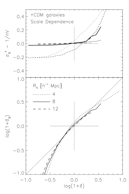
Figure 30: Same as figure 28, for galaxies with $M_{B}-5\log h\leq-19.5$.

Figure 32: Biasing characteristics as a function of smoothing scale for halos of $M\geq 10^{12}\mbox{$h^{-1}$ $M_{\odot}$}$ or galaxies with $M_{B}-5\log h\leq-19.5$ at $z=0$. Details are as in figure 18.

Figure 34: Biasing characteristics as a function of redshift. The two cosmological models are analyzed with T8 smoothing, for halos of $M\geq 10^{12}\mbox{$h^{-1}$ $M_{\odot}$}$ or galaxies with $M_{B}-5\log h\leq-19.5$. Details are as in figure 18.

Figure 36: The auto-correlation function for halos ($M\geq 10^{12}\mbox{$h^{-1}$ $M_{\odot}$}$; left panels, light lines) or galaxies ($M_{B}-5\log h\leq-19.5$; right panels, light lines) and for the dark matter (bold lines) at different redshifts.

Figure 40: Mass dependence of halo biasing ($b_{\rm var}$) at $z=0$, $z=1$, and $z=3$. Solid lines are the predictions of the MW model. Dotted lines are results from the $\tau$CDM simulations without correction for shot-noise. Symbols are results from the simulations with a standard Poisson correction for shot-noise. Circles and the lowest set of lines are for $z=0$, diamonds and the middle set of lines for $z=1$, and triangles and the highest lines are for $z=3$.

Figure 42: Redshift evolution of biasing ($b_{\rm var}$) of galaxies ($M_{B}-5\log h\leq-19.5$; stars) and halos ($M\geq 10^{12}\mbox{$h^{-1}$ $M_{\odot}$}$; dots) in the simulations, compared with analytic models. The light solid lines show the predictions of the MW model, with the same mass threshold as the simulation halos. The dotted lines show the predictions of the galaxy-conserving model, for initial bias values typical of halos or galaxies at $z=3$ or galaxies at $z=1$ in our simulations (see text for details).

References

- Adelberger et al. (1998) Adelberger K., Steidel C., Giavalisco M., Dickinson M., Pettini M., Kellogg M., 1998, ApJ, in press, astro-ph/9804236
- Bagla (1998) Bagla J., 1998, MNRAS, 299, 417
- Bardeen et al. (1986) Bardeen J. M., Bond J. R., Kaiser N., Szalay A. S., 1986, ApJ, 304, 15 (BBKS)
- Benson et al. (1999) Benson A., Cole S., Frenk C., Baugh C., Lacey C., 1999 (astro-ph/9903343)
- Binney & Tremaine (1987) Binney J., Tremaine S., 1987, Galactic Dynamics. Princeton Univ. Press, Princeton, NJ
- Blanton et al. (1998) Blanton M., Cen R., Ostriker J., Strauss M., 1998, ApJ, submitted (astro-ph/9807029)
- Blanton et al. (1999) Blanton M., Cen R., Ostriker J., Strauss M., Tegmark M., 1999, ApJ, submitted (astro-ph/9903165)
- Bruzual & Charlot (1998) Bruzual G., Charlot S., 1998, in preparation
- Catelan et al. (1998) Catelan P., Lucchin F., Matarrese S., Porciani C., 1998, MNRAS, 297, 692
- Cen & Ostriker (1998) Cen R., Ostriker J., 1998, ApJ, submitted (astro-ph/9809370)
- Coles et al. (1998) Coles P., Lucchin F., Matarrese S., Moscardini L., 1998, MNRAS, 300, 183
- Colín et al. (1998) Colín P., Klypin A., Kravtsov A., Khokhlov A., 1998, ApJ, submitted (astro-ph/9809202)
- Connolly et al. (1995) Connolly A., Szalay A., Bershady M., Kinney A., Calzetti D., 1995, AJ, 110, 1071
- Davis et al. (1985) Davis M., Efstathiou G., Frenk C. S., White S. D. M., 1985, ApJ, 292, 371
- Dekel (1994) Dekel A., 1994, ARA&A, 32, 371
- Dekel (1999) Dekel A., 1999, in Ostriker A. D. . J., ed, Formation of Structure in the Universe. Cambridge Univ. Press, p. 250
- Dekel et al. (1997) Dekel A., Burstein D., White S., 1997, in Turok N., ed, Critical Dialogues in Cosmology. World Scientific, p. 175
- Dekel & Lahav (1998) Dekel A., Lahav O., 1998, ApJ, submitted, astro-ph/9806193
- Dekel & Rees (1987) Dekel A., Rees M., 1987, Nature, 326, 455
- Diaferio et al. (1998) Diaferio A., Kauffmann G., Colberg J., White S., 1998, MNRAS, submitted (astro-ph/9812009)
- Dressler (1980) Dressler A., 1980, ApJ, 236, 351
- Folkes et al. (1996) Folkes S., Lahav O., Maddox S., 1996, MNRAS, 283, 651
- Fry (1996) Fry J., 1996, ApJ, 461, 65
- Giovanelli et al. (1997) Giovanelli R., Haynes M., Da Costa L., Freudling W., Salzer J., Wegner G., 1997, ApJ, 477, L1
- Gross et al. (1998) Gross M. A. K., Somerville R. S., Primack J. R., Holtzman J., Klypin A., 1998, MNRAS, 301, 81
- Guzzo et al. (1997) Guzzo L., Strauss M., Fisher K., Giovanelli R., Haynes M., 1997, ApJ, 489, 37
- Hermit et al. (1996) Hermit S., Santiago B., Lahav O., Strauss M., Davis M., Dressler A., Huchra J., 1996, MNRAS, 283, 709
- Jenkins et al. (1998) Jenkins et al., 1998, ApJ, 499, 20
- Kaiser (1984) Kaiser N., 1984, ApJ, 284, L9
- Katz et al. (1998) Katz N., Hernquist L., Weinberg D., 1998, ApJ, submitted (astro-ph/9806257)
- Kauffmann et al. (1998a) Kauffmann G., Colberg J. M., Diaferio A., White S., 1998a, MNRAS, submitted, astro-ph/9805283
- Kauffmann et al. (1998b) Kauffmann G., Colberg J. M., Diaferio A., White S., 1998b, MNRAS, submitted, astro-ph/9809168
- Kauffmann et al. (1997) Kauffmann G., Nusser A., Steinmetz M., 1997, MNRAS, 286, 795
- Landy et al. (1996) Landy S., Szalay A., Koo D., 1996, ApJ, 460, 94
- Loveday et al. (1995) Loveday J., Maddox S., Efstathiou G., Peterson A., 1995, ApJ, 442, 457
- Magliocchetti et al. (1999) Magliocchetti M., Bagla J. S., Maddox S. J., Lahav O., 1999 (astro-ph/9902260)
- Mann et al. (1998) Mann R., Peacock J., Heavens A., 1998, MNRAS, 293, 209
- Matattese et al. (1997) Matattese S., Coles P., Lucchin F., Moscardini L., 1997, MNRAS, 286, 115
- Mo & White (1996) Mo H., White S., 1996, MNRAS, 282, 347 (MW)
- Mo et al. (1998) Mo H. J., Mao S., White S., 1998, MNRAS, 304, 175
- Moscardini et al. (1998) Moscardini L., Coles P., Lucchin F., Matarrese S., 1998, MNRAS, 299, 95
- Narayanan et al. (1998) Narayanan V., Berlind A., Weinberg D., 1998, ApJ, submitted (astro-ph/9812002)
- Peebles (1980) Peebles P., 1980, The Large-Scale Structure of the Universe. Princeton Univ. Press, Princeton, NJ
- Press & Schechter (1974) Press W., Schechter P., 1974, ApJ, 187, 425
- Scalo (1986) Scalo J., 1986, Fundam. Cosmic Phys., 11, 1
- Somerville et al. (1998) Somerville R., Lemson G., Kolatt T., Dekel A., 1998, MNRAS, submitted, astro-ph/9807277
- Steidel et al. (1998) Steidel C., Adelberger K., Dickinson M., Giavalisco M., Pettini M., Kellogg M., 1998, ApJ, 492, 428
- Strauss & Willick (1995) Strauss M., Willick G., 1995, Phys. Rep., 261, 271
- Tegmark & Bromley (1998) Tegmark M., Bromley B., 1998, ApJ, submitted (astro-ph/9809324)
- Tegmark & Peebles (1998) Tegmark M., Peebles P., 1998, ApJ, 500, 79
- Tucker et al. (1997) Tucker D. et al., 1997, MNRAS, 285, 5
- Tully et al. (1999) Tully R. B., Pierce M. J., Huang J.-S., Saunders W., Verheijen M., Witchalls P., 1999, AJ, 115, 2264
- Wang & Heckman (1996) Wang B., Heckman T., 1996, ApJ, 457, 645
- Wechsler et al. (1998) Wechsler R., Gross M., Primack J., Blumenthal G., Dekel A., 1998, ApJ, in press (astro-ph/9712141)
- Willmer et al. (1998) Willmer C., Da Costa N., Pellegrini P., 1998, AJ, 115, 869