Sunyaev-Zel’dovich Effect Derived Distances to the High-Redshift Clusters MS $0451.6-0305$ and Cl $0016+16$

Abstract

We determine the distances to the $z\simeq 0.55$ galaxy clusters MS $0451.6-0305$ and Cl $0016+16$ from a maximum likelihood joint fit to interferometric Sunyaev-Zel’dovich effect (SZE) and X-ray observations. We model the intracluster medium (ICM) using a spherical isothermal $\beta$ model. We quantify the statistical and systematic uncertainties inherent to these direct distance measurements, and we determine constraints on the Hubble parameter for three different cosmologies. For an $\mbox{$\Omega_{M}$}=0.3$, $\mbox{$\Omega_{\Lambda}$}=0.7$ cosmology, these distances imply a Hubble constant of $63^{+12}_{-9\phantom{0}}\,{}^{+21}_{-21}$ km s^-1 Mpc^-1, where the uncertainties correspond to statistical followed by systematic at 68% confidence. The best fit $H_{\circ}$ is 57 km s^-1 Mpc^-1 for an open $\mbox{$\Omega_{M}$}=0.3$ universe and 52 km s^-1 Mpc^-1 for a flat $\mbox{$\Omega_{M}$}=1$ universe.

1. Introduction

Analysis of Sunyaev-Zel’dovich effect (SZE) and X-ray data from a cluster of galaxies provides information that can be used to determine the distance to the cluster, independent of the extragalactic distance ladder. In the early seventies, Sunyaev and Zel’dovich (1970, 1972) suggested that cosmic microwave background (CMB) photons inverse Compton scattering off the electrons in the hot ($\sim 10$ keV) intracluster medium (ICM) trapped in the potential well of the cluster, would cause a small ($\lesssim 1$ mK) distortion in the CMB spectrum, now known as the Sunyaev-Zel’dovich effect (SZE). The distortion appears as a decrement for frequencies $\lesssim 218$ GHz ($\lambda\gtrsim 1.4$ mm) and as an increment for frequencies $\gtrsim 218$ GHz. The SZE signal is proportional to the pressure integrated along the line of sight through the cluster, $\Delta T\sim\int\!n_{e}T_{e}d\ell$, where $n_{e}$ is the electron density of the ICM and $T_{e}$ is the electron temperature. The X-ray surface brightness can be written as $S_{x}\sim\int\!n_{e}^{2}\mbox{$\Lambda_{e\mbox{\tiny H}}$}d\ell$ where $\Lambda_{e\mbox{\tiny H}}$ is the X-ray cooling function, which depends on temperature and metallicity. It was soon realized that one can determine the distance to the cluster by capitalizing on the different dependencies on density, $n_{e}$, with some assumptions about the geometry of the cluster. This is a direct distance based only on relatively simple cluster physics and not requiring any standard candles or rulers.

The SZE signal is weak and difficult to detect. The recent success of SZE observations is due to advances in instrumentation and observational strategy. Recent high signal-to-noise ratio detections have been made with single dish observations at radio wavelengths (Birkinshaw & Hughes 1994; Herbig et al. 1995; Myers et al. 1997; Hughes & Birkinshaw 1998), millimeter wavelengths (Holzapfel et al. 1997a, b; Pointecouteau et al. 1999) and submillimeter wavelengths (Lamarre et al. 1998; Komatsu et al. 1999). Interferometric observations have produced high quality images of the SZE (Jones et al. 1993; Grainge et al. 1993; Carlstrom et al. 1996, 1998; Saunders et al. 1999; Grainge et al. 1999). On the theoretical side, there is substantial literature on relativistic corrections to both the SZE (Rephaeli & Yankovitch 1997; Itoh et al. 1998; Challinor & Lasenby 1998; Nozawa et al. 1998a; Sazonov & Sunyaev 1998) and X-ray bremsstrahlung (Hughes & Birkinshaw 1998; Rephaeli & Yankovitch 1997; Nozawa et al. 1998b). To date, there are about a dozen estimates of $H_{\circ}$ based on combining X-ray and SZE data for individual clusters (see Birkinshaw 1999 for a comprehensive review).

Table 1Radio Point Sources

	RA	DEC	$F_{28.5}$	$F_{15}$	$F_{5}$	$F_{1.4}$
Field	(J2000)	(J2000)	(mJy)	(mJy)	(mJy)	(mJy)
MS 0451	$04\mbox{${}^{\mbox{h}}$}$ $54\mbox{${}^{\mbox{m}}$}$ $22\mbox{${}^{\mbox{s}}$}$	$-03^{\circ}$ $01\arcmin$ $26\arcsec$	1.88	$\cdots$	$\cdots$	14.9
Cl 0016	$00\mbox{${}^{\mbox{h}}$}$ $18\mbox{${}^{\mbox{m}}$}$ $31\mbox{${}^{\mbox{s}}$}$	$+16^{\circ}$ $20\arcmin$ $45\arcsec$	9.07	25.0	84.5	267

We present a new analysis, wherein we perform a joint maximum-likelihood fit to both interferometric SZE and X-ray data. This method takes advantage of the unique properties of interferometric SZE data, utilizing all the available image data on the ICM. This is the first time SZE and X-ray data have been analyzed jointly. We apply this method to observations of MS $0451.6-0305$ and Cl $0016+16$, massive clusters at redshift $z=0.55$ (Donahue & Stocke 1995; Carlberg et al. 1994) and $z=0.5455$ (Neumann & Bohringer 1997; Dressler & Gunn 1992), respectively.

We describe the data and reduction in § 2, the analysis method in § 3, and present the results and possible systematic uncertainties in § 4. Section 5 contains a discussion of the results and future prospects. All uncertainties are 68.3% confidence unless explicitly stated otherwise.

2. Observations and Data Reduction

2.1. Interferometric SZE Observations

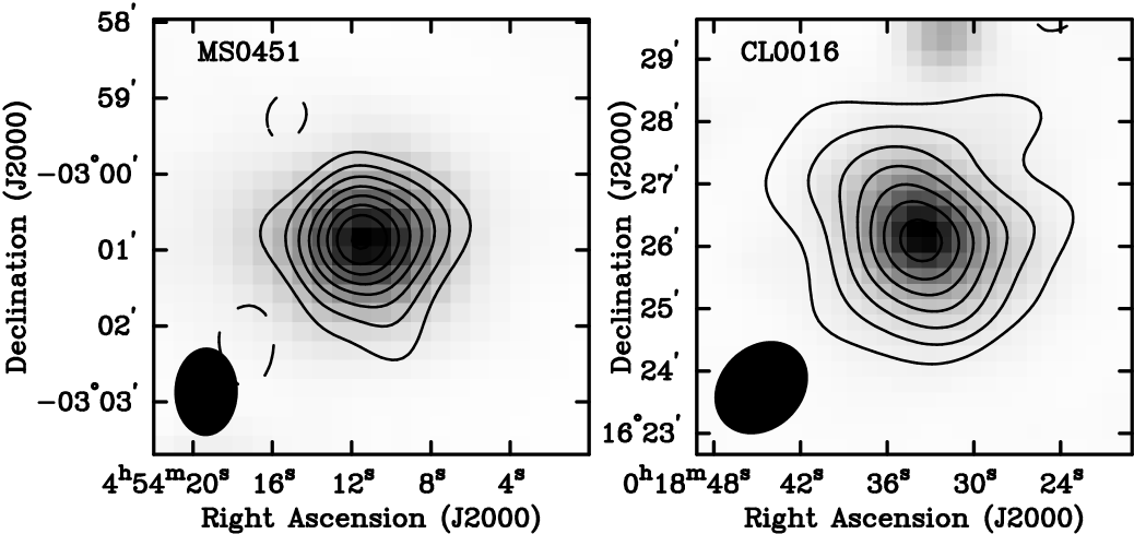
Figure 1.— SZE (contours) and X-ray (grey scale) image overlay for MS $0451.6-0305$ and Cl $0016+16$. The SZE images have an rms of $\sim 30$ $\mu$K (MS 0451) and $\sim 46$ $\mu$K (Cl 0016). The contours are multiples of 2 $\sigma$ and negative contours are shown as solid lines. The FWHM ellipse of the synthesized beam is shown in the lower left corner of each panel. The different sizes of the SZE images are due to the smaller dishes of the BIMA telescopes (used for Cl 0016) which can be more closely packed and thus sample smaller $u$-$v$ radii than the OVRO telescopes (used for MS 0451). The X-ray images are PSPC raw counts smoothed with a Gaussian with $\sigma=15\arcsec$. The peak for the MS 0451 image is 23 counts and 50 counts for the Cl 0016 image.

The extremely low systematics of interferometers and their two-dimensional imaging capability make them well suited to study the weak ($\lesssim 1$ mK) SZE signal in galaxy clusters. Over the past several summers, we outfitted the Berkeley Illinois Maryland Association (BIMA) millimeter array in Hat Creek, California, and the Owens Valley Radio Observatory (OVRO) millimeter array in Big Pine, California, with centimeter wavelength receivers. Our receivers use cooled ($\sim 10$ K) High Electron Mobility Transistor (HEMT) amplifiers (Pospieszalski et al. 1995) operating over 26-36 GHz with characteristic receiver temperatures of $T_{rx}\sim$11-20 K, over 28-30 GHz, the band used for the observations presented here. When combined with the BIMA or OVRO systems, these receivers obtain typical system temperatures scaled to above the atmosphere of $T_{sys}\sim 45$ K and as low as 34 K. Most telescopes are placed close together in a compact configuration to probe the angular scales subtended by distant clusters ($\sim$ 1′), but telescopes are always placed at longer baselines for simultaneous detection of point sources. Every half hour we observe a radio point source, commonly called a phase calibrator, to monitor the system gains for about two minutes.

MS 0451 was observed at OVRO in 1996 during May and June for 30 hours with six 10.4 m telescopes using two 1 GHz channels centered at 28.5 GHz and 30.0 GHz (2 GHz bandwidth). Cl 0016 was observed at OVRO in 1994 between June 16 and July 4 for 87 hours with five 10.4 m telescopes and a 1 GHz bandwidth centered at 28.7 GHz and in 1995 between July 24 and July 28 for 13 hours using five 10.4 m telescopes and two 1 GHz channels centered at 28.5 GHz and 30.0 GHz. Cl 0016 was also observed at BIMA in 1996 between September 6 and September 18 for 29 hours with six 6.1 m telescopes and in 1997 between June 21 and July 22 for 8 hours with nine 6.1 m telescopes, both years with an 800 MHz bandwidth centered at 28.5 GHz.

The data are reduced using the MIRIAD (Sault et al. 1995) software package at BIMA and using MMA (Scoville et al. 1993) at OVRO. In both cases, data are removed when one telescope shadows another, when cluster data are not straddled by two phase calibrators, when there are anomalous changes in instrumental response between calibrator observations, or when there is spurious correlation. For absolute flux calibration, we use observations of Mars, on the assumption that we know its true brightness temperature from the Rudy (1987) Mars model. For observations not containing Mars, calibrators in those fields are bootstrapped back to the nearest Mars calibration (see Grego 1999 for more details). The observations of the phase calibrators over each summer give us a summer-long calibration of the gains of the BIMA and OVRO interferometers. They both show very little gain variation, changing by less than 1% over a many-hour track, and the average gains remain stable from day to day.

An interferometer samples the Fourier transform of the sky brightness rather than the direct image of the sky. The final products from the interferometer are the amplitudes of the real and imaginary components of the Fourier transform of the cluster SZE distribution on the sky multiplied by the primary beam of the telescope. The SZE data files include the positions in the Fourier domain, which depend on the arrangement of the telescopes in the array, the real and imaginary components, and a measure of the noise in the real and imaginary components. The Fourier conjugate variables to right ascension and declination are commonly called $u$ and $v$, respectively, and the Fourier domain is commonly referred to as the $u$-$v$ plane.

The finite size of each telescope dish imposes an almost Gaussian attenuation across the field of view, known as the primary beam. The primary beams are constructed from holography data taken at each array. The main lobe of the primary beams can be approximated as Gaussian with a full width at half maximum (FWHM) of $4\arcmin.2$ for OVRO and $6\arcmin.6$ for BIMA at 28.5 GHz. We use the primary beam profiles made from the holography data for our analysis.

The primary beam sets the field of view. The effective resolution, called the synthesized beam, depends on the sampling of the $u$-$v$ plane of the observation and is therefore a function of the configuration of the telescopes. The cluster SZE signal is largest on the shortest baselines (largest angular scales). The shortest possible baseline is set by the diameter of the telescopes, $D$. Thus we are not sensitive to angular scales larger than about $\lambda/2D$, which is $\sim 2\arcmin.8$ for BIMA observations and $\sim 1\arcmin.7$ for OVRO observations. The compact configuration used for our observations yields significant SZE signal at these angular scales, but the interferometer is not sensitive to larger angular scales. Because of this spatial filtering by the interferometer, it is necessary to fit models directly to the data in the $u$-$v$ plane, rather than to the deconvolved image.

Point sources are identified from SZE images created with DIFMAP (Pearson et al. 1994) using only the long baseline data ($\gtrsim 2000\ \lambda$) and natural weighting. Approximate positions and fluxes for each point source are obtained from this image and used as inputs for the model fitting discussed in § 3.2. The data are separated by observatory, frequency, and by year to allow for temporal and spectral variability of the point source flux. One point source is found in both the MS 0451 and Cl 0016 fields. The point source positions and fluxes are from the model fitting described in § 3.2 and summarized in Table 1. Our positions agree very well with the NRAO VLA Sky Survey (NVSS) source positions (Condon et al. 1998).

The MS 0451 field point source is located 172″ from the pointing center with a measured flux of $0.50^{+0.07}_{-0.07}$ mJy at 28.5 GHz. Correcting for the primary beam attenuation appropriate for this offset, the intrinsic point source flux is $1.88^{+0.26}_{-0.26}$ mJy. In the 30 GHz channel, this point source has a flux of $0.36^{+0.07}_{-0.07}$ mJy, and $1.35^{+0.26}_{-0.26}$ after correcting for the primary beam. This point source was found in the NVSS survey with a flux of 14.9 mJy at 1.4 GHz (Condon et al. 1998). The point source in the Cl 0016 field is 339″ from the pointing center and is only seen in the BIMA data since the OVRO primary beam attenuation places it out of the OVRO field of view. The flux of this source is measured to be $1.01^{+0.23}_{-0.20}$ mJy at 28.5 GHz from the 1997 BIMA data, which when corrected for the primary beam attenuation, is an intrinsic flux of $9.07^{+2.07}_{-1.80}$. This source corresponds to source 15 from the survey of this field done by Moffet & Birkinshaw (1989). They found this source to be $267\pm 3$ mJy at 1.44 GHz (264 mJy in the more recent NVSS survey; Condon et al. 1998), $84.5\pm 1.1$ mJy at 4.86 GHz, and $25.0\pm 1.5$ mJy at 14.94 GHz. We do not see the other two sources of Moffet & Birkinshaw (1989) within 360″ of the pointing center, sources 10 and 14 which have 15 GHz fluxes of 0.56 and $<2.7$ mJy, respectively. We do not present a flux for the point source in the 1996 BIMA Cl 0016 data because of a problem with the absolute calibration of the array during observations early that summer. Though the overall normalization is uncertain, the data still provide shape information about the cluster. Table 1 summarizes the positions of the point sources and their fluxes at various frequencies.

Figure 1 shows the SZE image contours overlaid on the X-ray images of these clusters. We use DIFMAP (Pearson et al. 1994) to produce the naturally weighted SZE images. The point sources are subtracted from the data and a Gaussian taper applied to emphasize brightness variations on cluster scales before the image is deconvolved (CLEANed). For the MS 0451 OVRO data, we apply a 1200 $\lambda$ half-power radius Gaussian taper before deconvolving the image. This yields an elliptical Gaussian fit of $48\arcsec\times 70\arcsec$ for the synthesized beam (effective resolution) and a rms of $\sim 68$ $\mu$Jy beam^-1, corresponding to a Rayleigh-Jeans (RJ) brightness sensitivity of $\sim 30$ $\mu$K. For Cl 0016 we use the 1996 and 1997 BIMA data with a 1000 $\lambda$ half-power radius Gaussian taper giving a $81\arcsec\times 101\arcsec$ synthesized beam and a rms of $\sim 250$ $\mu$Jy beam^-1, corresponding to a $\sim 46$ $\mu$K RJ brightness sensitivity. The SZE image contours are multiples of twice the rms level for each image. Images made with the 1994 OVRO Cl 0016 data were presented in Carlstrom, Joy, & Grego (1996).

We stress that these images are made to demonstrate the data quality. The actual analysis is done in the Fourier plane, where the noise characteristics of the data and the spatial filtering of the interferometer are well understood. The SZE and X-ray image overlays in Figure 1 show that the region of the cluster sampled by the interferometric SZE observations and the X-ray observations is similar.

2.2. X-ray Observations

We use archival Röntgen Satellite (ROSAT) data from both the Position Sensitive Proportional Counter (PSPC) and High-Resolution Imager (HRI) instruments. MS 0451 was observed with the PSPC in 1993 over March 5-7 for 15,439 s of live-time and by the HRI in 1995 over September 3-19 for 45,864 s of live-time. There are approximately 1200 cluster photons collected in both the PSPC and HRI observations. Cl 0016 was observed with the PSPC in 1992 over July 11-18 for a live-time of 41,589 s and by the HRI in 1995 between June 17 and July 5 for a live-time of 70,228 s. The PSPC data contains about 3200 cluster photons and the HRI has about 1500.

We use the Snowden Extended Source Analysis Software (ESAS) (Snowden et al. 1994; Snowden 1998) to reduce the data. We use this software to generate a raw counts image, a noncosmic background image, and an exposure map for the HRI (0.1-2.4 keV) data and for each of the Snowden bands R4-R7 (PI channels $52-201$; approximately $0.5-2.0$ keV) for the PSPC data, using a master veto rate (a measure of the cosmic-ray and $\gamma$-ray backgrounds) of 200 counts s^-1 for the PSPC data. We examine the light curve data of both instruments looking for periodic, anomalously high count rates (short-term enhancements) and for periods of high scattered solar X-ray contamination. None are found. The Snowden software produces $512\times 512$ pixel images with $14.947\arcsec$ pixels for the PSPC and $5.0\arcsec$ pixels for the HRI. For the PSPC, final images for all of the R4-R7 bands together are generated by adding the raw counts images and the background images. Each Snowden band has a slightly different effective exposure map and there is an energy dependence in the point spread function (PSF). Thus, we generate a single exposure image and a single PSF image by combining cluster photon-weighted averages of the four exposure images and the four PROS (Worrall et al. 1992; Conroy et al. 1993) generated on-axis PSF images. The cluster photon-weighting is determined using the background subtracted detected photons within a circular region centered on the cluster. The region selected to construct the weights is the largest circular region encompassing the cluster which contains no bright point sources. For MS 0451, we use a 12 pixel radius and for Cl 0016 we use a 15 pixel radius. X-ray images with SZE image overlays of MS 0451 and Cl 0016 are shown in Figure 1. The gray-scale images are the PSPC “raw” counts images smoothed with a Gaussian with $\sigma=15\arcsec$. The peaks of the images are 23 counts (MS 0451) and 50 counts (Cl 0016).

For MS 0451, we use the emission-weighted temperature, galactic absorption, and metallicity from Donahue (1996). She found a best-fit X-ray temperature of $T_{e}=10.4^{+1.0}_{-0.8}$ keV with a galactic absorption column density of $\mbox{$N_{\mbox{\tiny H}}$}=3.0^{+0.4}_{-0.3}\times 10^{20}$ cm^-2 and a metallicity of $0.15^{+0.07}_{-0.07}$ solar implied by the iron abundance from a joint analysis of ASCA and PSPC data. This temperature is consistent with the Mushotzky & Scharf (1997) value of $T_{e}=10.17^{+0.93}_{-0.76}$ keV. For Cl 0016, we adopt the Hughes and Birkinshaw (1998) results. They found $T_{e}=7.55^{+0.72}_{-0.58}$ keV with a galactic absorption column density of $\mbox{$N_{\mbox{\tiny H}}$}=5.59^{+0.41}_{-0.36}\times 10^{20}$ cm^-2 and a metallicity of $0.07^{+0.11}_{-0.07}$ solar from a joint analysis of ASCA and PSPC data. This temperature agrees with a more recent analysis by Furuzawa et al. (1998) who found $T_{e}=8.0^{+0.6}_{-0.5}$ keV. Unlike the Hughes & Birkinshaw analysis, this analysis did not include the PSPC data which is sensitive to the column density.

2.2.1 X-ray Cooling Function

The Raymond-Smith (1977) code calculates the electron-ion bremsstrahlung contribution in the non-relativistic limit using the Gaunt factors of Karzas & Latter (1961). Recently it has been pointed out (Rephaeli & Yankovitch 1997; Hughes & Birkinshaw 1998) that relativistic corrections are important for a precise determination of angular diameter distances, and therefore also of $H_{\circ}$. Though dubbed “relativistic” corrections, the corrections go beyond only relativistic effects and include 1) relativistic corrections to the electron distribution function, 2) relativistic and spin corrections to the non-relativistic electron-ion bremsstrahlung cross section, 3) inclusion of electron-electron bremsstrahlung (all three of relative order $\mbox{$k_{\mbox{\tiny B}}$}T_{e}/m_{e}c^{2}$), and 4) first-order Born approximation corrections to electron-ion bremsstrahlung (of order $(Ry/\mbox{$k_{\mbox{\tiny B}}$}T_{e})^{1/2}$, where $Ry=13.6$ eV is the ionization energy of hydrogen). When applied, these corrections provide a better than 1% accurate calculation of thermal bremsstrahlung (Gould 1980). Gould provides results for both the integrated energy-loss rate and the spectral cooling function from thermal bremsstrahlung.

Following Hughes & Birkinshaw (1998), we use the corrections to the spectral cooling function rather than the total energy-loss rate used by Rephaeli & Yankovitch (1997) because the calculated cooling function comes from integrating the spectral cooling function over the fairly narrow ROSAT energy band redshifted to the cluster frame. These corrections may also affect the $T_{e}$ derived from fits to X-ray spectral data because these corrections modify the shape of the X-ray spectrum. Hughes & Birkinshaw (1998) found a $\sim 1$% change in the best fit $T_{e}$ for the Coma cluster ($T_{e}\sim 8$ keV) when applying these corrections to their spectral fits. As a check we also verified that the spectral cooling function formula from Gould when integrated over energy agrees with the total energy-loss result.

Table 2X-ray Cooling Functions for the PSPC

	$\Lambda_{e\mbox{\tiny H}\circ}$	$\Lambda_{e\mbox{\tiny H}\circ}^{\mbox{\tiny det}}$	$\Sigma$
Cluster	(erg s-1 cm3)	(cnt s-1 cm5)	($\frac{\mbox{erg s}^{-1}\mbox{ cm}^{-2}}{\mbox{cnt s}^{-1}}$)
MS 0451	$6.95\times 10^{-24}$	$3.26\times 10^{-13}$	$1.37\times 10^{-11}$
Cl 0016	$6.91\times 10^{-24}$	$3.00\times 10^{-13}$	$1.49\times 10^{-11}$

To calculate the X-ray spectral cooling function, we use a Raymond-Smith (1993 Sep 21 version) thermal plasma model with its bremsstrahlung component replaced with Gould’s bremsstrahlung calculation including the corrections discussed above. We use the Anders & Grevesse (1989) meteoritic abundances as the solar values, scaling the abundances of elements heavier than He by the metallicity of the cluster. We calculate the absorption from cold Galactic gas using the photoelectric cross sections from Balucinska-Church & McCammon (1992) (including the updated He absorption; 1993 Sep 23 version) for Anders & Grevesse solar abundances.

We integrate the modified Raymond-Smith spectral model over the redshifted ROSAT band (0.5-2.0 keV in the detector frame) to determine the cooling function in cgs units, $\Lambda_{e\mbox{\tiny H}\circ}$. We also calculate the cooling function in detector units by multiplying the modified Raymond-Smith spectrum by the response (includes effective area and energy resolution) of the instrument, dividing by the energy of the photons (to convert to counts), and integrating to find the total cooling function, $\Lambda_{e\mbox{\tiny H}\circ}^{\mbox{\tiny det}}$. Comparing these two yields the detector to cgs unit conversion, $\Sigma$, after correcting by $(1+z)$ due to the difference between instrument counts and energy ($\Sigma=\mbox{$\Lambda_{e\mbox{\tiny H}\circ}$}/\Lambda_{e\mbox{\tiny H}\circ}^{\mbox{\tiny det}}/(1+z)$). The cooling function results for the PSPC are summarized in Table 2. The cooling functions are 1.052 and 1.046 times the Raymond-Smith “uncorrected” value for MS 0451 and Cl 0016, respectively.

3. Method

3.1. Angular Diameter Distance Calculation

The calculation begins by constructing a model for the cluster gas distribution. We use a spherical isothermal $\beta$ model to describe the ICM. Within this context the cluster’s characteristic scale along the line of sight is the same as the scale in the plane of the sky. This model is clearly invalid in the presence of cluster asphericities. Thus cluster geometry introduces an important uncertainty in SZE and X-ray derived distances. In general, clusters are dynamically young, are aspherical, and rarely exhibit projected gas distributions which are circular on the sky (Mohr et al. 1995). We currently can not disentangle the complicated cluster structure and projection effects, but numerical simulations provide a good base for understanding these difficulties. The effects of asphericity contribute significantly to the distance uncertainty for each cluster, but do not result in any significant bias in the Hubble parameter derived from a large sample of clusters (Sulkanen 1999; Mohr et al. 1999a).

The spherical isothermal $\beta$ model is given by (Cavaliere & Fusco-Femiano 1976, 1978)

$$n_{e}({\mathbf{r}})=\mbox{$n_{e\circ}$}\left(1+\frac{r^{2}}{r_{c}^{2}}\right)^{-3\beta/2},$$ (1)

where $n_{e}$ is the electron number density, $r$ is the radius from the center of the cluster, $r_{c}$ is the core radius of the ICM, and $\beta$ is the power law index. With this model, the SZE signal is

$$\Delta T = f_{(x)}\mbox{$T_{\mbox{\tiny CMB}}$}\mbox{$D_{\!\mbox{\tiny A}}$}\!\int\!\!d\zeta\,\mbox{$\sigma_{\mbox{\tiny T}}$}n_{e}\frac{\mbox{$k_{\mbox{\tiny B}}$}T_{e}}{m_{e}c^{2}}$$ (2)

$$= \mbox{$\Delta T_{\circ}$}\left(1+\frac{\theta^{2}}{\theta_{c}^{2}}\right)^{(1-3\beta)/2},$$

where $\Delta T$ is the SZE decrement/increment, $f_{(x)}=\mbox{$(x\frac{e^{x}+1}{e^{x}-1}-4)(1+\delta_{\mbox{\tiny SZE}})$}$ ($f_{(x)}\rightarrow-2$ in the non-relativistic and Rayleigh-Jeans limits) is the frequency dependence of the SZE with $x=h\nu/k\mbox{$T_{\mbox{\tiny CMB}}$}$, $\delta_{\mbox{\tiny SZE}}(x,T_{e})$ is the relativistic correction to the frequency dependence, $T_{\mbox{\tiny CMB}}$ (=2.728 K; Fixsen et al. 1996) is the temperature of the CMB radiation, $k_{\mbox{\tiny B}}$ is the Boltzmann constant, $\sigma_{\mbox{\tiny T}}$ is the Thompson cross section, $m_{e}$ is the mass of the electron, $c$ is the speed of light, $\Delta T_{\circ}$ is the central SZE decrement/increment, $\theta$ is the angular radius in the plane of the sky and $\theta_{c}$ the corresponding angular core radius, and the integration is along the line of sight $\ell=\mbox{$D_{\!\mbox{\tiny A}}$}\zeta$. We apply the relativistic corrections $\delta_{\mbox{\tiny SZE}}$ to fifth order in $kT_{e}/m_{e}c^{2}$ (Itoh et al. 1998). The Itoh et al. results agree with other work (Stebbins 1997; Challinor & Lasenby 1998) to third order where they stop. This correction decreases the magnitude of $f_{(x)}$ by 3.7% for MS 0451 and 2.7% for Cl 0016. The correction is slightly higher for MS 0451, as expected, because of its higher electron temperature.

The X-ray surface brightness is

$$S_{x} = \frac{1}{4\pi(1+z)^{4}}\mbox{$D_{\!\mbox{\tiny A}}$}\!\int\!\!d\zeta\,n_{e}\mbox{$n_{\mbox{\tiny H}}$}\mbox{$\Lambda_{e\mbox{\tiny H}}$}\>\;\!$$ (3)

$$= \mbox{$S_{x\circ}$}\left(1+\frac{\theta^{2}}{\theta_{c}^{2}}\right)^{(1-6\beta)/2},$$

where $S_{x}$ is the X-ray surface brightness in cgs units (erg s^-1 cm^-2 arcmin^-2), $z$ is the redshift of the cluster, $n_{\mbox{\tiny H}}$ is the hydrogen number density of the ICM, $\mbox{$\Lambda_{e\mbox{\tiny H}}$}=\mbox{$\Lambda_{e\mbox{\tiny H}}$}(T_{e},\mbox{abundance})$ is the X-ray cooling function of the ICM in the cluster rest frame in cgs units (erg cm³ s^-1) integrated over the redshifted ROSAT band, and $S_{x\circ}$ is the X-ray surface brightness in cgs units at the center of the cluster. Since the X-ray observations are in instrument counts, we also need the conversion factor between detector counts and cgs units, $\Sigma$, discussed in §2.2.1 ($\mbox{$S_{x\circ}$}=S_{x\circ}^{\mbox{\tiny det}}\Sigma$). The normalizations, $\Delta T_{\circ}$ and $S_{x\circ}$, used in the fit include all of the physical parameters and geometric terms that come from the integration of the $\beta$ model along the line of sight.

One can solve for the angular diameter distance by eliminating $n_{e\circ}$ (noting that $\mbox{$n_{\mbox{\tiny H}}$}=n_{e}\mu_{e}/\mbox{$\mu_{\mbox{\tiny H}}$}$ where $n_{j}\equiv\rho/\mu_{j}m_{p}$ for species $j$) yielding

$$\mbox{$D_{\!\mbox{\tiny A}}$}=\frac{(\mbox{$\Delta T_{\circ}$})^{2}}{\mbox{$S_{x\circ}$}}\left(\frac{m_{e}c^{2}}{\mbox{$k_{\mbox{\tiny B}}$}\mbox{$T_{e\circ}$}}\right)^{2}\frac{\mbox{$\Lambda_{e\mbox{\tiny H}\circ}$}\mu_{e}/\mbox{$\mu_{\mbox{\tiny H}}$}}{4\pi^{3/2}\,f_{(x)}^{2}\,T_{\mbox{\tiny CMB}}^{2}\,\sigma_{\mbox{\tiny T}}^{2}\,(1+z)^{4}}$$

$$\times\frac{1}{\theta_{c}}\left[\frac{\Gamma(\frac{3}{2}\beta)}{\Gamma(\frac{3}{2}\beta-\frac{1}{2})}\right]^{2}\frac{\Gamma(3\beta-\frac{1}{2})}{\Gamma(3\beta)}$$ (4)

where $\Gamma(x)$ is the Gamma function. Similarly, one can eliminate $D_{\!\mbox{\tiny A}}$ instead and solve for the central density $n_{e\circ}$.

3.2. Joint SZE and X-ray Model Fitting

The SZE and X-ray emission both depend on the properties of the ICM, so a joint fit to all the available data provides the best constraints on those properties. We perform a joint fit to the interferometric SZE data and the PSPC and HRI X-ray data. Each data set is assigned a collection of parameterized models. Typically, SZE data sets are assigned a $\beta$ model and point sources and X-ray images are assigned a $\beta$ model and a cosmic X-ray background model. This set of models is combined for each data set to create a composite model which is then compared to the data.

Model parameters can be fixed, free to find their optimized values, or gridded. They can also be linked, forced to vary together among the data sets. In practice, $\theta_{c}$ and $\beta$ are linked between all data sets (both SZE and X-ray) and the central decrements $\Delta T_{\circ}$ are linked between the SZE data sets which are separated by season and array. We use a downhill simplex to search parameter space and maximize the joint likelihood (Press et al. 1992). The cluster position, $\beta$, $\theta_{c}$, $S_{x\circ}$, $\Delta T_{\circ}$, a constant cosmic background, radio point source positions, and point source fluxes are all allowed to vary.

Each data set is independent, and likelihoods from each data set can simply be multiplied together to construct the joint likelihood. Likelihood ratio tests can then be performed to get confidence regions or compare two models. Rather than working directly with likelihoods, $\mathcal{L}$, we work with $S\equiv-2\ln(\mathcal{L})$. We then construct a $\Delta\chi^{2}$-like statistic from the log likelihoods, $\Delta S\equiv S_{n}-S_{ref}$ where $S_{ref}$ is the reference $S$ statistic, typically chosen to be the minimum of the $S$ function, and $S_{n}$ is the $S$ statistic where $n$ parameters differ from the parameters at the reference. The statistic $\Delta S$ is sometimes referred to as the Cash (1979) statistic and tends to a $\chi^{2}$ distribution with $n$ degrees of freedom (Kendall & Stuart 1979 for example). This $\Delta S$ statistic is equivalent to the likelihood ratio test and is used to generate confidence regions and confidence intervals with $S_{ref}=S_{min}$. For one interesting parameter, the 68.3% ($\sim 1\sigma$) confidence level corresponds to $\Delta S=1.0$.

Because we are interested only in differences in log likelihoods, $\Delta S$, the model independent terms in the likelihoods are dropped. The log likelihoods are then

$$\sum_{i}-\frac{1}{2}\left(\Delta R^{2}_{i}+\Delta I^{2}_{i}\right)W_{i} \mbox{for SZE data (Gaussian)},$$ (5)

$$\sum_{i}D_{i}\ln(M_{i})-M_{i}\ \ \ \ \ \ \>\, \mbox{for X-ray data (Poisson)},$$ (6)

where $\Delta R_{i}$ and $\Delta I_{i}$ are the differences between the model and data at each point $i$ in the Fourier plane for the real and imaginary components respectively, $W_{i}=1/\sigma_{i}^{2}$ is a measure of the noise (Gaussian) of the real and imaginary components discussed in §2.1, and $M_{i}$ and $D_{i}$ are the model prediction and data in pixel $i$.

Figure 2.— Comparison of the PSPC radially averaged surface brightness profile (points with error bars) with the best fitting isothermal spherical $\beta$-model plus background (histogram) for a) MS 0451 and b) Cl 0016. The lower panel shows the residuals in units of the standard deviation. The best fit model is a good fit to the data over the entire range of radii considered in the fit. There is no evidence of excess emission near the core for either cluster, the signature of cooling flows.

The interferometric SZE observations provide constraints in the Fourier ($u$-$v$) plane, so we perform our model fitting in the $u$-$v$ plane, where the noise properties of the data and the spatial filtering of the interferometer are well defined. The SZE composite model for both MS 0451 and Cl 0016 consists of a $\beta$ model and a point source. The $\beta$ model is computed in a regular grid in image space, multiplied by the primary beam determined from holography measurements, and fast Fourier transformed to produce the $u$-$v$ plane model. It is then interpolated to the $u$-$v$ position for each data point. Point sources are computed analytically at each $u$-$v$ data point of the observation and added to the $\beta$ model in the $u$-$v$ plane to construct the composite SZE model. The Gaussian likelihood (eq. [5]) is calculated using the composite SZE model and the SZE data. During the fitting, the cluster center, $\theta_{c}$, $\beta$, $\Delta T_{\circ}$, the point source positions, and the point source fluxes are all allowed to vary.

Because the SZE is frequency dependent, a minor additional detail comes from observations of a cluster at multiple frequencies, 28.5 GHz and 30 GHz. We input a central decrement appropriate for 30 GHz into the fitting routine, which then corrects the model for the actual frequency of the observation. The likelihood is calculated with the model appropriate for the observing frequency. This allows us to link the central decrement across data sets with different observing frequencies.

Table 3ICM Parameters

		$\theta_{c}$	$S_{x\circ}^{\mbox{\tiny det}}$	$S_{x\circ}$	$\Delta T_{\circ}$
Cluster	$\beta$	(arcsec)	(cnt s-1 arcmin-2)	(erg s-1 cm-2 arcmin-2)	($\mu$K)
MS 0451	$0.806^{+0.052}_{-0.043}$	$34.7^{+3.9}_{-3.5}$	$6.96^{+0.63}_{-0.61}$ $\times 10^{-2}$	$9.56^{+0.86}_{-0.84}$ $\times 10^{-13}$	$-1431^{+\phantom{0}98}_{-\phantom{0}93}$
Cl 0016	$0.749^{+0.024}_{-0.018}$	$42.3^{+2.4}_{-2.0}$	$4.14^{+0.16}_{-0.19}$ $\times 10^{-2}$	$6.17^{+0.24}_{-0.28}$ $\times 10^{-13}$	$-1242^{+105}_{-105}$

The model for each X-ray data image includes a spherical isothermal $\beta$ model plus a constant cosmic background. The model is convolved with the appropriate PSF, multiplied with the exposure map, and then the noncosmic background is added pixel by pixel. Point sources are masked out. The logarithm of the Poisson likelihood (eq. [6]) is then calculated. During the fitting, the cluster center, $\theta_{c}$, $\beta$, $S_{x\circ}$, and the cosmic background are all allowed to vary. The PSF is generated by PROS and the exposure map and noncosmic background maps are those generated by the Snowden ESAS software discussed in § 2.2. The PSF and exposure maps for the PSPC Snowden bands R4-R7 are combined in a cluster photon-weighted average (see § 2.2). Point sources are found using the ESAS detection algorithm with a 3 $\sigma$ detection criterion and masked out. Circular regions of typically 3 pixel radius are placed on each point source and excluded from the calculation of the likelihood. These regions correspond to radii of $\sim 45\arcsec$ for the PSPC and $15\arcsec$ for the HRI. As a check, the image of the cluster excluding the masked regions is visually inspected. Increasing the size of the masked regions does not significantly alter the best fit parameters, including the cosmic background. For the model fitting we use a region centered on the cluster with a 64 pixel radius, corresponding to $\sim 16\arcmin$ for the PSPC and $\sim 5\arcmin$ for the HRI. Using a larger fitting region does not change the best fit model parameters significantly.

When allowed to vary separately, the best-fit central surface brightnesses for the PSPC and HRI are consistent within their uncertainties when compared in cgs units. We linked the central surface brightnesses between the PSPC and HRI in cgs units, using $\Sigma$ to convert to counts before comparing with the X-ray images. The linked $S_{x\circ}$ case gives an insignificant change in the $S$ statistic compared to the case where the PSPC and HRI normalizations are allowed to vary individually and removes one free parameter. The consistent central surface brightnesses from the PSPC and HRI observations present an interesting test of the relative calibration of the two instruments.

4. Direct Distances and the Hubble Constant

The results from our maximum likelihood joint fit to the SZE and X-ray data are summarized in Table 3 for both clusters. Figures 2a and 2b show the X-ray radial surface brightness profiles and the best fit composite models for MS 0451 and Cl 0016, respectively. The models for both clusters show a good fit to the data over a large range of angular radii. Using equation (4) with the best-fit parameters from Table 3 and the cooling functions from Table 2, we find the distance to MS 0451 to be $1278^{+265}_{-298}$ Mpc and the distance to Cl 0016 to be $2041^{+484}_{-514}$ Mpc, where the uncertainties are statistical only (see discussion below).

Our fitting results are consistent with previous analyses of the ROSAT data of MS 0451 and Cl 0016. Donahue (1996) analyzed the MS 0451 PSPC data and found $\beta=1.01^{+0.27}_{-0.18}$ and $\theta_{c}=38.2^{+11.6}_{-\phantom{0}9.6}$ arcseconds. Table 4 shows the comparison for Cl 0016 with Neumann & Böhringer (1997) and Hughes & Birkinshaw (1998).

Table 4Comparison of Cl 0016 Analyses

			$\theta_{c}$
Reference	Instrument	$\beta$	(arcsec)
NB97	PSPC	$0.80\phantom{0}^{+0.04}_{-0.05}$	$50.5^{+4.5}_{-4.0}$
NB97	HRI	$0.68\phantom{0}^{+0.10}_{-0.07}$	$38.5^{+8.0}_{-6.5}$
HB98	PSPC	$0.728^{+0.025}_{-0.022}$	$40.7^{+2.7}_{-2.3}$
This work	joint PSPC & HRI	$0.749^{+0.024}_{-0.018}$	$42.3^{+2.4}_{-2.0}$

We also compare our results with the distance determination to Cl 0016 by Hughes & Birkinshaw (1998). They analyzed the PSPC observations to determine the ICM shape parameters and then used that model to extract the SZE central decrement from observations taken with the OVRO single dish 40 m telescope at 20.3 GHz. They observed seven points in a north-south scan through Cl 0016. Beam switching was done using the 40 m dual-beam system, which provides two 1′.78 FWHM beams separated by 7′.15 in azimuth. The central decrement extracted from such scans depends on the adopted center of the SZE signal as well as the adopted ICM shape parameters, $\beta$ and $\theta_{c}$. Interferometric observations provide two-dimensional imaging information with accurate astrometry and therefore provide information about the cluster center and the ICM shape parameters. We find a central decrement of $-1242^{+105}_{-105}$ $\mu$K remarkably consistent with the Hughes & Birkinshaw value of $-1201^{+189}_{-189}$ $\mu$K converted to thermodynamic temperature at 30 GHz. Hughes & Birkinshaw found the distance to Cl 0016 to be $1863^{+836}_{-549}$ Mpc in good agreement with ours, where the uncertainty is statistical only and we have corrected for the frequency dependence of the SZE ($f_{(x)}\neq-2$) and relativistic corrections. Our PSPC central surface brightness and cooling function are both lower than the Hughes & Birkinshaw values. This difference arises entirely from using a different bandpass for the analysis ($0.5-2.0$ keV versus $0.4-2.4$ keV). However, only the ratio of the surface brightness and cooling function enters into the distance calculation. Our ratio times $\mu_{H}/\mu_{e}$ ($\Lambda_{e\mbox{\tiny H}}$ versus $\Lambda_{ee}$) is $1.65\times 10^{11}$ arcmin^-2 cm^-5 in fortuitously good agreement with theirs, $1.64\times 10^{11}$ arcmin^-2 cm^-5.

Table 5$D_{\!\mbox{\tiny A}}$ Observational Uncertainty Budget (percent)

Cluster	Fit	$N_{\mbox{\tiny H}}$	$[\mbox{Fe}]/[\mbox{H}]$	$T_{e}$	Total
MS 0451	${}^{+13.7}_{-13.1}$	${}^{+0.9}_{-1.2}$	${}^{+1.1}_{-1.1}$	${}^{+15.4}_{-19.2}$	${}^{+20.7}_{-23.3}$
Cl 0016	${}^{+17.8}_{-16.4}$	${}^{+1.1}_{-1.2}$	${}^{+2.1}_{-1.3}$	${}^{+15.4}_{-19.1}$	${}^{+23.7}_{-25.2}$

There is a known correlation between the $\beta$ and $\theta_{c}$ parameters of the $\beta$ model. One might think this correlation would make determinations of $D_{\!\mbox{\tiny A}}$ imprecise because $D_{\!\mbox{\tiny A}}$ is calculated from these very shape parameters of the ICM. Figure 4 illustrates this correlation and its effect on $D_{\!\mbox{\tiny A}}$ for MS 0451. The filled contours are the 1, 2, and 3 $\sigma$ $\Delta S$ confidence regions for $\beta$ and $\theta_{c}$ jointly. The lines are contours of constant $D_{\!\mbox{\tiny A}}$ in Mpc. With our interferometric SZE data, the contours of constant $D_{\!\mbox{\tiny A}}$ lie roughly parallel                                                                  

Confidence regions from the joint SZE and X-ray fit for MS 0451. The filled regions are 1, 2, and 3 sigma confidence regions for $\beta$ and $\theta_{c}$ jointly ($\Delta S=$ 2.3, 6.2, 11.8) and the cross marks the best fit $\beta$ and $\theta_{c}$. Solid lines are contours of angular diameter distance in Mpc. The $D_{\!\mbox{\tiny A}}$ contours lie roughly parallel to the $\beta$-$\theta_{c}$ correlation, minimizing the effect of this correlation on the uncertainties of $D_{\!\mbox{\tiny A}}$.

to the $\beta$-$\theta_{c}$ correlation, minimizing the effect of this correlation on the uncertainties of $D_{\!\mbox{\tiny A}}$. Figure 4 shows similar behavior for Cl 0016. Different observing techniques will result in different behavior. Contours of constant $D_{\!\mbox{\tiny A}}$ have been found to be roughly orthogonal to the $\beta$-$\theta_{c}$ correlation for some single dish SZE observations (Birkinshaw & Hughes 1994; Birkinshaw et al. 1991).

Uncertainties in the angular diameter distance from the fit parameters are calculated by gridding in the interesting parameters to explore the $\Delta S$ likelihood space. The most important parameters in this calculation are $\Delta T_{\circ}$, $S_{x\circ}$, $\beta$, and $\theta_{c}$. Radio point sources and the cosmic X-ray background affect $\Delta T_{\circ}$ and $S_{x\circ}$, respectively. Therefore we grid in $\Delta T_{\circ}$, $S_{x\circ}$, $\beta$, and $\theta_{c}$ allowing the X-ray backgrounds for the PSPC and HRI to float independently. To estimate the effect of the radio point sources, we find the best-fit parameter values with the point source flux fixed at its best fit value. We also run the grids for the point source flux fixed at the $\pm 1\ \sigma$ values. The point sources in the MS 0451 and Cl 0016 fields are both far enough from the cluster center so that their flux contributions have   a                                                                  

Same as Figure 4 for Cl 0016.

negligible effect on the central decrement and do not change the cluster shape parameters significantly. From this four dimensional $\Delta S$ hyper-surface, we construct confidence intervals for each parameter individually as well as confidence intervals for $D_{\!\mbox{\tiny A}}$ due to $S_{x\circ}$, $\Delta T_{\circ}$, $\beta$, and $\theta_{c}$ jointly. The correlations between the $\beta$ model parameters require this treatment to determine accurately the uncertainty in $D_{\!\mbox{\tiny A}}$ from the fitted parameters. To compute the 68.3% confidence region we find the minimum and maximum values of the parameter within a $\Delta S$ of 1.0. We emphasize that these uncertainties are meaningful only within the context of the spherical isothermal $\beta$ model.

Table 6$H_{\circ}$ Systematic Uncertainty Budget for MS 0451 and Cl 0016

Systematic	Effect
	(%)
SZE calibration	$\pm\phantom{0}8$
X-ray calibration	$\pm 10$
$N_{\mbox{\tiny H}}$	$\pm\phantom{0}5$
Asphericity	$\pm 14$
Isothermality & clumping	$\pm 20$
Undetected radio sources	$\pm 16$
Kinetic SZE	$\pm\phantom{0}6$
Total	$\pm 33$

The observational uncertainty budget for $D_{\!\mbox{\tiny A}}$ is shown in Table 5. The uncertainties in the fitted parameters come from the above procedure. The only other parameter that enters directly into the $D_{\!\mbox{\tiny A}}$ calculation is $T_{e\circ}$. Since $\mbox{$D_{\!\mbox{\tiny A}}$}\propto\mbox{$T_{e\circ}$}^{-2}$, the uncertainty in $D_{\!\mbox{\tiny A}}$ due to $T_{e\circ}$ is listed as twice the fractional uncertainty on $T_{e\circ}$. The other parameters, column density and metallicity, as well as $T_{e\circ}$, affect the X-ray cooling function. We estimate the uncertainties in $D_{\!\mbox{\tiny A}}$ due to these parameters by taking their 68.3% ranges and seeing how much they affect the cooling function. The uncertainty in the cooling function due to $T_{e\circ}$ is $\lesssim 0.5$% and is ignored. The uncertainty on $D_{\!\mbox{\tiny A}}$ due to observations is dominated by the uncertainty in the electron temperature and the SZE central decrement. Note that changes of factors of two in metallicity result in a $\sim 1$% effect on $D_{\!\mbox{\tiny A}}$. The column densities measured from the X-ray spectra are different from those from H I surveys (Dickey & Lockman 1990). We use the column densities from X-ray spectral fits since that includes contributions from nonneutral hydrogen and other elements which absorb X-rays. The survey derived column densities change the angular diameter distance by $\sim\pm 5$%, which we include as a systematic uncertainty (see § 5).

To determine the Hubble Constant, we perform a $\chi^{2}$ fit to our calculated $D_{\!\mbox{\tiny A}}$’s versus $z$ for three different cosmologies. To estimate statistical uncertainties, we combine the uncertainties on $D_{\!\mbox{\tiny A}}$ listed in Table 5 in quadrature, which is only strictly valid for Gaussian distributions. This combined statistical uncertainty is symmetrized (averaged) and used in the fit. We find

$$\mbox{$H_{\circ}$}=\cases{52^{+10}_{-\phantom{0}7}\ \mbox{km s${}^{-1}$ Mpc${}^{-1}$};&\mbox{$\Omega_{M}$}=1.0, \mbox{$\Omega_{\Lambda}$}=0.0,\cr 57^{+11}_{-\phantom{0}8}\ \mbox{km s${}^{-1}$ Mpc${}^{-1}$};&\mbox{$\Omega_{M}$}=0.3, \mbox{$\Omega_{\Lambda}$}=0.0,\cr 63^{+12}_{-\phantom{0}9}\ \mbox{km s${}^{-1}$ Mpc${}^{-1}$};&\mbox{$\Omega_{M}$}=0.3, \mbox{$\Omega_{\Lambda}$}=0.7,\cr}$$ (7)

where the uncertainties are statistical only. The statistical error comes from the $\chi^{2}$ analysis and includes uncertainties from $T_{e}$, the parameter fitting, metallicity, and $N_{\mbox{\tiny H}}$ (see Table 5). We have chosen three cosmologies encompassing the currently favored models. There is a $\sim 20$% range in $H_{\circ}$ at $z\sim 0.5$ due to the geometry of the universe.

4.1. Sources of Possible Systematic Uncertainty

The absolute calibration of both the SZE observations and the PSPC and HRI directly affects the distance determinations. The absolute calibration of the interferometric observations is conservatively known to about 4% at 68% confidence, corresponding to a 8% uncertainty in $H_{\circ}$ ($\propto\Delta T_{\circ}^{-2}$). The effective areas of the PSPC and HRI are thought to be known to about 10%, introducing a 10% uncertainty into the $H_{\circ}$ determination through the calculation of $\Sigma$. In addition to the absolute calibration uncertainty from the observations, there are possible sources of systematic uncertainty that depend on the physical state of the ICM and other sources that can contaminate the cluster SZE emission. Table 6 summarizes the systematic uncertainties in the Hubble constant determined from MS 0451 and Cl 0016.

4.1.1 Cluster Atmospheres and Morphology

Most clusters do not appear circular in radio, X-rays, or optical. Fitting a projected elliptical isothermal $\beta$ model gives an axial ratio of $\sim 0.80$ and $\sim 0.84$ for MS 0451 and Cl 0016, respectively, close to the local average of $0.80$ (Mohr et al. 1995). Under the assumption of axisymetric clusters, the combined effect of cluster asphericity and its orientation on the sky conspires to introduce a $\sim\pm 20$% random uncertainty in $H_{\circ}$ (Hughes & Birkinshaw 1998). When one considers a large, unbiased sample of clusters, presumably with random orientations, the uncertainty due to imposing a spherical model will cancel, manifesting itself in the statistical uncertainty and allowing a precise determination of $H_{\circ}$. Recently, Sulkanen (1999) studied projection effects using triaxial $\beta$ models. Fitting these with spherical models he found that the Hubble constant estimated from the fitting was within $\simeq 5$% of the true value. We are in the process of using N-body and smoothed particle hydrodynamics (SPH) simulations of 48 clusters to quantify the effects of complex cluster structure on our results.

Cooling flows also affect the derived distance to the cluster, affecting the emission weighted mean temperature and enhancing the X-ray central surface brightness (see, e.g., Nagai et al. 2000). A characteristic cooling time for the ICM is

$$t_{cool}\sim\frac{3kT_{e}n_{tot}}{2\Lambda n_{e}\mbox{$n_{\mbox{\tiny H}}$}}=\frac{3kT_{e}}{2\Lambda n_{e}}\frac{\mbox{$\mu_{\mbox{\tiny H}}$}}{\mu_{tot}},$$ (8)

where $\Lambda$ is the bolometric cooling function of the cluster and all quantities are evaluated at the center of the cluster. Cooling flows may occur if the cooling time is less than the age of the cluster, which we conservatively estimate to be the age of the universe at the redshift of observation, $t_{cool}<t_{H}(z)$. For a flat, Einstein-de Sitter universe, the Hubble time is $t_{H}(z)=\frac{2}{3}\mbox{$H_{\circ}$}^{-1}(1+z)^{-3/2}$. Both MS 0451 and Cl 0016 are observed in the $z\approx 0.55$ universe so that $t_{H}(z=0.55)=3\times 10^{9}\;h^{-1}$ years. The ratio of the cooling time to the Hubble time for typical ICM parameters at redshift of 0.55 is then

$$\frac{t_{cool}}{t_{H}(z=0.55)}\sim 19h\left(\frac{T_{e}}{8\mbox{ keV}}\right)\left(\frac{2.5\times 10^{-23}\ \mbox{erg cm${}^{3}$ s${}^{-1}$}}{\Lambda}\right)$$

$$\times\left(\frac{10^{-3}\mbox{ cm}^{-3}}{n_{e}}\right).\ \ \ \$$ (9)

Using the best fit parameters we find $\Lambda=2.8\times 10^{-23}$ erg cm³ s^-1 and $n_{e}=1.3\times 10^{-2}$ cm^-3 for MS 0451 and $\Lambda=2.4\times 10^{-23}$ erg cm³ s^-1 and $n_{e}=7.0\times 10^{-3}$ cm^-3 for Cl 0016 (the densities are determined by eliminating $D_{\!\mbox{\tiny A}}$ in eqs. [2] and [3] in favor of $n_{e\circ}$). This implies $t_{cool}/t_{H}$ ratios of $\sim 1.7$ and $\sim 2.6$ respectively. These ratios are summarized in Table 7 for all three cosmologies considered in this paper. From this simple calculation, we do not expect cooling flows in either of these clusters. The X-ray radial surface brightness profiles (Figs 2a and b) provide no evidence for excess emission in the cluster core (see also Donahue & Stocke 1995; Neumann & Bohringer 1997). As a check, we calculate $t_{cool}/t_{H}$ ratios for each cluster analyzed by Mohr et al. (1999). We check our cooling flow and non-cooling flow determinations versus those of Peres et al. (1998) and Fabian (1994). Of the 45 clusters in the Mohr sample, 41 have published mass deposition rates. We assume the cluster does not contain a cooling flow if its mass deposition rate is consistent with zero, otherwise it is designated as a cooling flow cluster. We are able to predict whether a cluster has a cooling flow or not with a 90% success rate, suggesting that the ratio $t_{cool}/t_{H}$ presented in equation (9) is a good predictor for the presence of a cooling flow.

Table 7Ratio of $t_{cool}/t_{H}(z)$

	Cosmology($\Omega_{M}$, $\Omega_{\Lambda}$)
Cluster	(1.0, 0.0)	(0.3, 0.0)	(0.3, 0.7)
MS 0451	1.7	1.3	1.0
Cl 0016	2.6	1.9	1.6

An isothermal analysis of a non-isothermal cluster could result in a large distance error; moreover, an isothermal analysis of a large cluster sample could lead to systematic errors in the derived Hubble parameter if most clusters have similar departures from isothermality (Birkinshaw & Hughes 1994; Inagaki et al. 1995; Holzapfel et al. 1997b). The effects of temperature variations depend on the observing technique. For example, PSPC X-ray constraints on the ICM distribution are very insensitive to temperature variations for gas whose temperatures are above 1.5 keV (see Fig. 1, Mathiesen et al. 1999). In principle, SZE observations are sensitive to temperature variations, because the SZE decrement is proportional to the projected pressure distribution (see eq. [2]). However, interferometric observations of the type presented here are relatively insensitive to modest ICM temperature variations.

Interferometric SZE observations sample the Fourier transform of the sky brightness distribution over a limited region of the $u$-$v$ plane. Specifically, the radio telescope dish size imposes a minimum separation for any two telescopes, making it impossible to sample the Fourier transform of the cluster SZE below some minimum radius in the $u$-$v$ plane. Moreover, the primary beam of the telescope defines some effective field of view, making interferometric observations completely insensitive to sky brightness fluctuations on any angular scale for those regions of the sky which lie outside the field of view. For these reasons interferometric SZE observations are insensitive to large angular scale variations in sky brightness. Therefore, clusters whose core regions are approximately isothermal and whose ICM temperatures decrease only gradually toward the virial region pose no problems for an isothermal analysis.

We are currently analyzing mock observations of gas-dynamical cluster simulations to explore the effects of expected temperature distributions for our observing strategy. These simulated clusters exhibit X-ray merger signatures consistent with those observed in real clusters and, presumably, they exhibit the appropriate complexities in their temperature structure as well. Preliminary results from this analysis indicate that expected temperature gradients do not introduce a large systematic error in our distance measurements. However, clumping within the ICM due to the common mergers of subclusters does enhance the X-ray surface brightness by $\sim 20$%. This enhancement causes X-ray gas mass estimates to be biased high by 10% (Mohr et al. 1999b), and it results in a $\sim 20$% underestimate of cluster distances. There is currently no direct observational evidence of clumping within the ICM, but merger signatures are common (Mohr et al. 1995), and the mergers are the driving mechanism behind these fluctuations in the simulated clusters (Mathiesen et al. 1999). We conservatively include a 20% systematic for clumping and departures from isothermality.

4.1.2 Possible SZE Contaminants

Undetected point sources may bias the angular diameter distance. Point sources near the cluster center mask the SZE decrement, causing an underestimate in the magnitude of the decrement, and therefore an underestimate of the angular diameter distance. While we can not rule out point sources below our detection threshold, to estimate an upper bound on their effects we add a point source with flux at our detection limit near the cluster center to each data set and then fit the new data set, not accounting for the added point source. Such a point source being at the cluster center is highly unlikely but provides an upper bound to the effects of undetected point sources. For a point source with flux density 1, 2, and 3 times the rms ($\sim 65$ $\mu$Jy) in the high-resolution ($\gtrsim 1,800\lambda$) image for MS 0451, we find the magnitude of the decrement decreases by 3%, 8%, and 14% respectively. For the Cl 0016 high-resolution image ($\gtrsim 1,500\lambda$), we find the decrement changes by 2%, 10%, and 17% for an on-center point source with flux density 1, 2, and 3 times the rms ($\sim 90$ $\mu$Jy) respectively. However, we can place more stringent constraints on contamination from undetected point sources because we have information about the distribution of point sources in these two fields from observations at lower frequencies. By performing a deeper survey of these fields with our 30 GHz receivers with an array configured for higher resolution we can lower our point source detection threshold until the uncertainty from undetected point sources becomes negligible.

The NVSS (Condon et al. 1998) detected two point sources within 400″ from the center of MS 0451. Of these, we detect the one that is 170″ from the pointing center, but the point source 295″ from the pointing center is outside the OVRO field of view. Sources with flux densities greater than $\sim 4\;\sigma\approx 2$ mJy appear in their catalog. As a more realistic upper bound on the contamination from undetected point sources, we extrapolate a point source with flux density equal to 4 $\sigma$ at 1.4 GHz to 28.5 GHz using the average spectral index of radio sources in galaxy clusters $\alpha=0.77$ (Cooray et al. 1998). Therefore, we place a 180 $\mu$Jy point source near the center of MS 0451 and then fit the new image, not accounting for the additional point source. The magnitude of the central decrement decreases by 13% which is a reasonable upper bound to the contamination from undetected point sources in the MS 0451 field and similar to the constraints derived from our own data.

Moffet & Birkinshaw (1989) surveyed the region around Cl 0016 at 5 GHz with the VLA and then followed up the 5 GHz sources at 1.4 GHz and 15 GHz. Three of their sources (10, 14, and 15) fall within the BIMA field of view. We detect source 15 in the BIMA data, but it falls outside the OVRO field of view at 338″ from the pointing center. We extrapolate sources 10 and 14 to 28.5 GHz from the 1.4 GHz observations using the spectral index $\alpha=0.77$, which is consistent with the Moffet & Birkinshaw result, $\alpha=0.7$. After correction for the primary beam, sources 10 and 14 are expected to be 28 $\mu$Jy and 227 $\mu$Jy, respectively. We add these two point sources to the OVRO data placing them at their NVSS positions, perform a model fit not accounting for them, and find a 3% change in the central decrement. Moffet & Birkinshaw searched for peaks that were 5$\sigma$ or greater. Extrapolating the 5 GHz rms of 80 $\mu$Jy to 28.5 GHz results in a 21 $\mu$Jy rms. Placing a 5$\sigma$ (100 $\mu$Jy) point source near the cluster center decreases the magnitude of the central decrement by 3%, identical to the combined effect from sources 10 and 14.

Cluster peculiar velocities with respect to the CMB introduce an additional CMB spectral distortion known as the kinetic SZE. The kinetic SZE is proportional to the thermal effect but has a different spectral signature so it can be disentangled from the thermal SZE with spectral SZE observations. For a 10 keV cluster with a line-of-sight peculiar velocity of 1000 km s^-1, the kinetic SZE is $\sim 11$% of the thermal SZE at 30 GHz. Watkins (1997) presented observational evidence suggesting a one-dimensional rms peculiar velocity of $\sim 300$ km s^-1 for clusters, and recent simulations found similar results (Colberg et al. 2000). With a line-of-sight peculiar velocity of 300 km s^-1 and a more typical 8 keV cluster, the kinetic SZE is $\sim 4$% of the thermal effect, introducing up to a $\sim\pm 8$% correction to the angular diameter distance computed from one cluster. The effects from peculiar velocities when averaged over an ensemble of clusters should cancel, manifesting itself as an additional statistical uncertainty similar to the effects of asphericity.

CMB primary anisotropies have the same spectral signature as the kinetic SZE. Recent BIMA observations provide limits on primary anisotropies on the scales of the observations presented here (Holzapfel et al. 2000). We place a 95% confidence upper limit to the primary CMB anisotropies of $\Delta T<22$ $\mu$K at $\ell\sim 5500$ ($\sim 2\arcmin$ scales). Thus primary CMB anisotropies are an unimportant ($\lesssim 2$%) source of uncertainty for our observations.

5. Discussion and Conclusions

We perform a maximum-likelihood joint fit to interferometric SZE and ROSAT X-ray (PSPC and HRI) data to constrain the ICM parameters for MS 0451 and Cl 0016. We model the ICM as a spherical, isothermal $\beta$ model. From this analysis we determine the distances to be $1278^{+265}_{-298}$ Mpc and $2041^{+484}_{-514}$ Mpc for MS 0451 and Cl 0016, respectively (statistical uncertainties only). Together, these distances imply a Hubble constant of

$$\mbox{$H_{\circ}$}=\cases{52^{+10}_{-\phantom{0}7}\,{}^{+17}_{-17}\ \mbox{km s${}^{-1}$ Mpc${}^{-1}$};&\mbox{$\Omega_{M}$}=1.0, \mbox{$\Omega_{\Lambda}$}=0.0,\cr 57^{+11}_{-\phantom{0}8}\,{}^{+19}_{-19}\ \mbox{km s${}^{-1}$ Mpc${}^{-1}$};&\mbox{$\Omega_{M}$}=0.3, \mbox{$\Omega_{\Lambda}$}=0.0,\cr 63^{+12}_{-\phantom{0}9}\,{}^{+21}_{-21}\ \mbox{km s${}^{-1}$ Mpc${}^{-1}$};&\mbox{$\Omega_{M}$}=0.3, \mbox{$\Omega_{\Lambda}$}=0.7,\cr}$$ (10)

where the uncertainties are statistical followed by systematic at 68% confidence. The systematic uncertainties have been added in quadrature and include an 8% (4% in $\Delta T_{\circ}$) uncertainty from the absolute calibration of the SZE data, a 10% effective area uncertainty for the PSPC and HRI, a 5% uncertainty from the column density, a 14% ($\simeq 20/\sqrt{2}$) uncertainty due to asphericity, a 20% effect for our assumptions of isothermality and single-phase gas, a 16% (8% in $\Delta T_{\circ}$) uncertainty from undetected radio sources, and a 6% ($\simeq 8/\sqrt{2}$) uncertainty from the kinetic SZE. These systematic uncertainties are summarized in Table 6. The uncertainty from undetected radio sources is the average of the maximum effects due to undetected sources for the MS 0451 (26%) and Cl 0016 (6%) fields. The contributions from asphericity and kinetic SZE should average out for a large sample.

Our $H_{\circ}$ determination from high-redshift clusters is consistent with other SZE based measurements as well as the recent results from the Hubble Space Telescope (HST) $H_{\circ}$ Key Project, which probed the nearby universe and found $\mbox{$H_{\circ}$}=71\pm 6$ km s^-1 Mpc^-1 (Mould et al. 2000). Birkinshaw (1999) compiled current SZE based $H_{\circ}$ measurements and found an ensemble average of $\sim 60$ km s^-1 Mpc^-1 independent of the chosen cosmology; where the uncertainty is difficult to ascertain because the measurements are not independent, many share SZE or X-ray data, and nearly all share common absolute calibrations.

The SZE derived distances are direct, making them an interesting check of the cosmological distance ladder. Recent observations of masers orbiting the nucleus of the nearby galaxy NGC4258 (Herrnstein et al. 1999) illustrate a method of determining direct distances in the nearby universe. Time delays from analysis of gravitational lensing data from galaxy clusters are another direct distance indicator that can probe the high redshift universe (for recent examples see Fassnacht et al. 1999; Biggs et al. 1999; Lovell et al. 1998; Barkana 1997; Schechter et al. 1997). The redshift independence of the SZE makes it a powerful probe of clusters at high redshift. The combination of SZE and deep X-ray observations could provide a valuable independent check of high redshift SN Ia results (Schmidt et al. 1998; Perlmutter et al. 1999), which constrain the geometry of the universe.

We are currently analyzing a larger sample of SZE clusters which will reduce the statistical uncertainty as well as effects from asphericity and the kinetic SZE. Analysis of mock observations of simulated clusters will also provide insight into the effects of temperature gradients and multiphase ICMs. With the recent launch of Chandra and the impending launch of XMM, we will soon obtain better $T_{e}$ measurements (currently a large source of observational uncertainty; see Table 5) and measure temperature profiles. In addition, the $\sim 2$% absolute calibration uncertainty of Chandra will soon replace the $\sim 10$% ROSAT absolute calibration uncertainty. There is also work being done to improve the absolute calibration at 30 GHz using the planets. The goal is to achieve a $\lesssim 1$% absolute calibration, further reducing the systematic uncertainties in the derived Hubble parameter.

References

- Anders & Grevesse (1989) Anders, E. & Grevesse, N. 1989, Geochim. Cosmochim. Acta, 53, 197
- Balucinska-Church & McCammon (1992) Balucinska-Church, M. & McCammon, D. 1992, ApJ, 400, 699
- Barkana (1997) Barkana, R. 1997, ApJ, 489, 21
- Biggs et al. (1999) Biggs, A. D., Browne, I. W. A., Helbig, P., Koopmans, L. V. E., Wilkinson, P. N., & Perley, R. A. 1999, MNRAS, 304, 349
- Birkinshaw (1999) Birkinshaw, M. 1999, Physics Reports, 310, 97
- Birkinshaw & Hughes (1994) Birkinshaw, M. & Hughes, J. P. 1994, ApJ, 420, 33
- Birkinshaw et al. (1991) Birkinshaw, M., Hughes, J. P., & Arnaud, K. A. 1991, ApJ, 379, 466
- Carlberg et al. (1994) Carlberg, R. G. et al. 1994, JRASC, 88, 39
- Carlstrom et al. (1998) Carlstrom, J. E., Grego, L., Holzapfel, W. L., & Joy, M. 1998, Eighteenth Texas Symposium on Relativistic Astrophysics and Cosmology, ed A. Olinto, J. Frieman, and D. Schramm, World Scientific, 261
- Carlstrom et al. (1996) Carlstrom, J. E., Joy, M., & Grego, L. 1996, ApJ, 456, L75
- Cash (1979) Cash, W. 1979, ApJ, 228, 939
- Cavaliere & Fusco-Femiano (1976) Cavaliere, A. & Fusco-Femiano, R. 1976, A&A, 49, 137
- Cavaliere & Fusco-Femiano (1978) —. 1978, A&A, 70, 677
- Challinor & Lasenby (1998) Challinor, A. & Lasenby, A. 1998, ApJ, 499, 1
- Colberg et al. (2000) Colberg, J. M., White, S. D. M., MacFarland, T. J., Jenkins, A., Pearce, F. R., Frenk, C. S., Thomas, P. A., & Couchman, H. M. P. 2000, MNRAS– submitted: astro-ph/9805078
- Condon et al. (1998) Condon, J. J., Cotton, W. D., Greisen, E. W., Yin, Q. F., Perley, R. A., Taylor, G. B., & Broderick, J. J. 1998, AJ, 115, 1693
- Conroy et al. (1993) Conroy, M. A., Deponte, J., Moran, J. F., Orszak, J. S., Roberts, W. P., & Schmidt, D. 1993, in ASP Conf. Ser. 52: Astronomical Data Analysis Software and Systems II, Vol. 2, 238
- Cooray et al. (1998) Cooray, A. R., Grego, L., Holzapfel, W. L., Joy, M., & Carlstrom, J. E. 1998, AJ, 115, 1388
- Dickey & Lockman (1990) Dickey, J. M. & Lockman, F. J. 1990, ARA&A, 28, 215
- Donahue (1996) Donahue, M. 1996, ApJ, 468, 79
- Donahue & Stocke (1995) Donahue, M. & Stocke, J. T. 1995, ApJ, 449, 554
- Dressler & Gunn (1992) Dressler, A. & Gunn, J. E. 1992, ApJS, 78, 1
- Fabian (1994) Fabian, A. C. 1994, ARA&A, 32, 277
- Fassnacht et al. (1999) Fassnacht, C. D., Pearson, T. J., Readhead, A. C. S., Browne, I. W. A., Koopmans, L. V. E., Myers, S. T., & Wilkinson, P. N. 1999, ApJ– in press: astro-ph/9907257
- Fixsen et al. (1996) Fixsen, D. J., Cheng, E. S., Gales, J. M., Mather, J. C., Shafer, R. A., & Wright, E. L. 1996, ApJ, 473, 576
- Furuzawa et al. (1998) Furuzawa, A., Tawara, Y., Kunieda, H., Yamashita, K., Sonobe, T., Tanaka, Y., & Mushotzky, R. 1998, ApJ, 504, 35
- Gould (1980) Gould, R. J. 1980, ApJ, 238, 1026
- Grainge et al. (1993) Grainge, K., Jones, M., Pooley, G., Saunders, R., & Edge, A. 1993, MNRAS, 265, L57
- Grainge et al. (1999) Grainge, K., Jones, M. E., Pooley, G., Saunders, R., Edge, A., & Kneissl, R. 1999, MNRAS–submitted: astro-ph/9904165
- Grego (1999) Grego, L. 1999, PhD thesis, Caltech
- Herbig et al. (1995) Herbig, T., Lawrence, C. R., Readhead, A. C. S., & Gulkis, S. 1995, ApJ, 449, L5
- Herrnstein et al. (1999) Herrnstein, J. R. et al. 1999, Nature, 400, 539
- Holzapfel et al. (1997a) Holzapfel, W. L., Ade, P. A. R., Church, S. E., Mauskopf, P. D., Rephaeli, Y., Wilbanks, T. M., & Lange, A. E. 1997a, ApJ, 481, 35
- Holzapfel et al. (1997b) Holzapfel, W. L. et al. 1997b, ApJ, 480, 449
- Holzapfel et al. (2000) Holzapfel, W. L., Carlstrom, J. E., Grego, L., Holder, G. P., Joy, M., & Reese, E. D. 2000, ApJ–submitted: astro-ph/9912010
- Hughes & Birkinshaw (1998) Hughes, J. P. & Birkinshaw, M. 1998, ApJ, 501, 1
- Inagaki et al. (1995) Inagaki, Y., Suginohara, T., & Suto, Y. 1995, PASJ, 47, 411
- Itoh et al. (1998) Itoh, N., Kohyama, Y., & Nozawa, S. 1998, ApJ, 502, 7
- Jones et al. (1993) Jones, M. et al. 1993, Nature, 365, 320
- Karzas & Latter (1961) Karzas, W. J. & Latter, R. 1961, ApJS, 6, 167
- Kendall & Stuart (1979) Kendall, M. & Stuart, A. 1979, in New York: Macmillan, 246
- Komatsu et al. (1999) Komatsu, E., Kitayama, T., Suto, Y., Hattori, M., Kawabe, R., Matsuo, H., Schindler, S., & Yoshikawa, K. 1999, ApJ, 516, L1
- Lamarre et al. (1998) Lamarre, J. M. et al. 1998, ApJ, 507, L5
- Lovell et al. (1998) Lovell, J. E. J., Jauncey, D. L., Reynolds, J. E., Wieringa, M. H., King, E. A., Tzioumis, A. K., McCulloch, P. M., & Edwards, P. G. 1998, ApJ, 508, L51
- Mathiesen et al. (1999) Mathiesen, B., Evrard, A. E., & Mohr, J. J. 1999, ApJ, 520, L21