Resolving Molecular Line Emission from Protoplanetary Disks: Observational Prospects for Disks Irradiated by Infalling Envelopes

Abstract

Molecular line observations that could resolve protoplanetary disks of $\sim 100$ AU both spatially and kinematically would be a useful tool to unambiguously identify these disks and to determine their kinematical and physical characteristics. In this work we model the expected line emission from a protoplanetary disk irradiated by an infalling envelope, addressing the question of its detectability with subarcsecond resolution. We adopt a previously determined disk model structure that gives a continuum spectral energy distribution and a mm intensity spatial distribution that are consistent with observational constraints of HL Tau. An analysis of the capability of presently working and projected interferometers at mm and submm wavelengths shows that molecular transitions of moderate opacity at these wavelengths (e.g., C${}^{17}$O lines) are good candidates for detecting disk lines at subarcsecond resolution in the near future. We suggest that, in general, disks of typical Class I sources will be detectable. Higher line intensities are obtained for lower inclination angles, larger turbulent velocities, and higher temperatures, with less effect from density changes.

The resulting maps show several characteristics that can be tested observationally. A clear asymmetry in the line intensity, with more intense emission in the disk area farther away from the observer, can be used to compare the geometrical relationship between disks and outflows. A decrease in intensity towards the center of the disk is also evident. Finally, the emission peaks in position velocity diagrams trace mid-plane Keplerian velocities.

1 Introduction

Circumstellar accretion disks around young stellar objects (YSOs) play a central role in our understanding of the stellar and planetary formation processes and related phenomena, which justifies the important efforts invested in their detection and characterization.

In the currently accepted paradigm, these accretion disks should appear naturally from the collapse of a core of molecular gas with a residual angular momentum. Theoretical models estimate that disks of radius $\sim 100$ AU should form around young low-mass stars (see, e.g., Terebey, Shu, & Cassen 1984; Morfill 1989). Gas and dust disks of sizes $\sim 100$ AU could give rise to planetary systems similar to ours. This is why these disks are usually referred to as “protoplanetary disks”.

The extensive search for protoplanetary disks that has taken place during the past years have provided astronomers with a large body of compelling evidence about their existence. Most of this evidence is indirect in the sense that it comes from observations that do not resolve the emission from the disk or that infer their existence from different phenomena in the gas and dust (e.g., Rodríguez et al. 1986; Adams, Shu, & Lada 1988; Bertout, Basri, & Bouvier 1988; Kenyon, Hartmann, & Hewett 1988; Keene & Masson 1990; Carr et al. 1993; O’Dell, Wen, & Hu 1993; Stauffer et al. 1994). A major difficulty to obtain a resolved image of a protoplanetary disk is that subarcsecond resolution is required (100 AU subtends 0$\farcs$7 at 140 pc, the distance to the closest known star-disk systems).

The most unambiguous identification of a disk, and the highest level of information about its physical parameters would probably be obtained with spectroscopic observations, with good enough angular resolution to resolve them, i.e, subarcsecond resolution. In addition to the morphological information that continuum observations can provide, spectroscopic observations would yield kinematical information from the gas in the disk, namely the kinematical signatures of rotation. Spectroscopic observations will also be a very powerful tool to determine the physical characteristics (e.g., densities and temperatures) of disks without requiring heavy modeling. If we can combine spectroscopic capabilities with subarcsecond resolution, we will then obtain a conclusive evidence for a structure to be considered a protoplanetary disk, and very accurate constraints on its physics.

Unfortunately, this kind of observations has not been possible so far with the current instrumentation. Important observational efforts have been devoted to obtain resolved continuum images of disks or unresolved spectroscopic data. Continuum observations have provided information on sizes and morphology of disks, as well as the relationship of these structures with outflow phenomena (e.g., Rodíguez et al. 1992, 1994; Lay et al. 1994; Mundy et al. 1996; Wilner, Ho, & Rodríguez 1996; McCaughream & O’Dell 1996; Burrows et al. 1996). On the other hand, spectroscopic data have provided kinematical information, and clues on the physical properties of disks, specially in the inner regions for the CO overtone emission (e.g., Hartmann & Kenyon 1987a, 1987b; Calvet et al. 1991;  Carr et al. 1993; Najita et al. 1996; Najita et al. 1999)

In practice, to obtain resolved spectroscopic data, one would probably have to pursue molecular line observations of disks using radio interferometers in the near future. First, because these instruments can achieve high angular resolutions. Second, because lines in disks with temperatures $\sim 100$ K (Beckwith et al. 1990) are more likely to be detected in the radio regime. And third, because the absorption due to molecular material external to the disk is lower at radio wavelengths.

Of course, the key question is whether it is possible to resolve and detect disks with sizes on the order of 100 AU, using molecular line observations. However, there are not many instruments that can reach subarcsecond resolution at present. One of the possibilities, using presently working instruments, was to observe inversion transitions of ammonia using the Very Large Array (VLA), whose B configuration have an angular resolution of $\sim 0\farcs 4$ for ammonia lines at 1.3 cm. This experiment was carried out by Gómez et al. (1993) toward HL Tau and L1551-IRS 5, but unfortunately it gave only upper limits. Looking into the future, we may wonder whether the resolving of protoplanetary disks will be possible with instruments now in project, for instance the Millimeter Array (MMA) of the National Radio Astronomy Observatory, the Submillimeter Array (SMA) of the Smithsonian Astrophysical Observatory, the Large Millimeter Array of the Nobeyama Radio Observatory, any possible upgrade of the present millimeter interferometers, the new VLA receivers at 7 mm (of which 13 are already working), etc (see Ho 1995).

To answer the question of the future detectability of protoplanetary disks, we have developed a model of their molecular line emission. In particular, this paper presents the case of an accretion disk irradiated by an infalling envelope, constructed to satisfy the observational constraints in continuum of HL Tau. There are several models of molecular line emission from protoplanetary disks that have been reported in the literature. These models have been developed essentially to compare with and to predict results of observations feasible with present telescopes, i.e., with beams $\geq 1^{\prime\prime}$ that do not resolve the disks. For instance, Beckwith & Sargent (1993), and Omodaka, Kitamura, & Kawazoe (1992) presented models of the emission of the rotational transitions of the CO isotopes at 3 mm, finding a double-peaked line profile, which is typical of rotating disks. In general, the comparison of these models with the observations gives good indirect evidence for the existence of these disks. There are also models for the emission of larger disk-like structures ($R\geq 1000$ AU) in Keplerian rotation, which also compare well with observations (e.g., GG Tau: Dutrey, Guilloteau, & Simon 1994; GM Aur: Koerner, Sargent, & Beckwith 1993). Although the sizes of these structures are about one order of magnitude larger than the actual accretion disks (which are believed to lie within these larger structures), these works are very important since they give good support to the theoretical expectation of the existence of rotating disks around young stellar objects. However, in some cases the interpretation of flattened structures of sizes on the order of 1000 AU as large rotating disks is not straightforward. For instance, the kinematics in the ${}^{13}$CO structure mapped in HL Tau (Sargent & Beckwith 1991; Hayashi, Ohashi, & Miyama 1993), could be dominated by an infalling flattened envelope (Hartmann et al. 1994; Hartmann, Calvet & Boss 1996), an infalling “pseudodisk” formed in the presence of a magnetic field (Galli & Shu 1993a,b; Hayashi et al. 1993), or entrainment in a bipolar outflow (Cabrit et al. 1996).

This paper addresses the problem of calculating the molecular line emission from protoplanetary disks (radius $\sim 100$ AU) expected when observing with an arbitrary angular resolution, especially the subarcsecond resolution necessary to resolve the disks. In this first work, we focus on the case of a disk irradiated by an infalling envelope. This would be the case for embedded sources, in an early stage of evolution. Apart from the radial dependence of density and temperature within the disk, we include, for the first time, a detailed vertical dependence of these parameters in the calculation of molecular line emission. In particular, we calculate molecular line profiles for the case of HL Tau, which is probably the disk source most extensively studied in the literature. The wealth of data from this source allow us to constrain the density and temperature structure (both radial and vertical) of its disk, mainly by fitting its continuum emission. From this structure, we computed the molecular line emission that, therefore, is consistent with the continuum emission. Thus, our calculations apply to a realistic source structure, that we can assume then as a good example of star-disk system in an early stage of evolution, still embedded in a substantial amount of circumstellar material. From our calculations we can have an estimate about whether the imaging of molecular line emission from this type of protoplanetary disks is possible with the telescopes presently available, or we have to wait for the advent of the next generation of radio interferometers to achieve such a goal.

The model presented here will be complemented with future similar studies using models for disks at different stages of evolution, like, for instance, optically visible T Tauri stars. In those cases, the properties of the envelope and the physical processes in the disk will produce a different density and temperature structure, which will affect line detectability and other observational properties. Those different models will require an individualized treatment.

2 Model for the Disk Structure in HL Tau

HL Tau is a classical T Tauri star with a strong excess emission at both optical-UV and far IR-radio wavelengths, which is still embedded in circumstellar material (Stapelfeld et al. 1995). The large infrared excess can be explained by emission from an infalling dusty envelope (Calvet et al. 1994, hereafter CHKW; Hartmann et al. 1996, hereafter HCB), which also reproduce other observational features like redshifted C${}_{2}$ optical absorption lines (Grasdalen et al. 1989), near infrared scattered light images (Beckwith, Koreski, & Sargent 1989) and the velocity pattern seen in the spatially-resolved ${}^{13}$CO map obtained with the Nobeyama Millimeter Array (Hayashi et al. 1993). However, the envelope surrounding HL Tau cannot account for the observed continuum flux at wavelengths longer than $\sim 1$ mm (CHKW, HCB).

On the other hand, a circumstellar disk can have enough column mass to explain the observed millimeter continuum emission of HL Tau, if the temperature in the outer regions of the disk is sufficiently high (Beckwith et al. 1990; Beckwith & Sargent 1991), with a dependency with distance to the star roughly $T\propto r^{-0.5}$. The interferometric observations of Lay et al. (1994, 1997) at $\lambda=0.65,0.87$ mm with the single baseline CSO-JCMT, Sargent & Koerner at $\lambda=1.4$ mm with OVRO (see Lay et al. 1997), Mundy et al. (1996) at 2.7 mm using BIMA, and Wilner, Ho, & Rodríguez (1996) at 7 mm using the VLA in its B configuration, indicate that the millimeter continuum emission is confined to small scales $R\lesssim 200$ AU, suggesting that it comes from a disk.

D’Alessio, Calvet, & Hartmann (1997, hereafter DCH) have developed models of steady accretion disks irradiated by optically thick infalling envelopes. In these models the structure of the disk (in both vertical and radial directions) is calculated in detail. The radiation from the rotating and infalling envelope is calculated from detailed envelope models (CHKW, HCB), in which the transfer equation is solved at each frequency including both scattering and emission by dust. The envelope calculations from CHKW and HCB assume that the luminosity comes from a star and a disk; in the case of HL Tau, $\sim$ 95% of the luminosity is estimated to originate from the disk.

DCH have shown that irradiation of a circumstellar disk by an optically-thick infalling envelope that reprocesses the disk radiation can quantitatively explain the high outer disk temperatures required by the submillimeter and millimeter observations of HL Tau. The envelope heating, determined by modeling completely independent constraints (the Spectral Energy Distribution (SED) between $1\mu$m $\lesssim\lambda\lesssim 100\mu$m; CHKW, HCB), dominates the outer disk temperature distribution.

The disk is assumed steady, geometrically thin, in vertical hydrostatic equilibrium and with a turbulent viscosity calculated using the standard $\alpha$ viscosity prescription (Shakura & Sunyaev 1973), i.e., the viscosity coefficient is expressed as $\nu=\alpha c_{\rm s}H$, where $c_{\rm s}$ is the local sound speed, $H$ is the local pressure scale height of the gas and $\alpha$ is the viscosity parameter (assumed constant throughout the disk). For an $\alpha$ disk, the surface density of mass $\Sigma$ is given by

$$\Sigma={\dot{M}\Omega_{K}\over 3\pi\alpha c_{s}^{2}(T_{c})}$$ (1)

where $\dot{M}$ is the disk mass accretion rate, $\Omega_{K}$ is the Keplerian angular velocity, and $T_{c}$ is the midplane temperature.

Since $\Sigma\propto T_{c}^{-1}$, the higher the midplane temperature (which is controlled by the envelope irradiation) the smaller the surface density. For the mm continuum, the opacity is dominated by dust and is independent on temperature. Thus, the continuum optical depth is $\tau_{\nu}\propto T_{c}^{-1}$, and the higher the envelope irradiation flux, the smaller the $\tau_{\nu}$. The source function at mm wavelengths is proportional to $T_{c}$. This means that as long as the envelope heats the $\alpha$ disk enough to make the outer regions ($R>50\ \rm AU$) optically thin in the mm continuum, the brightness temperature distribution in this spectral range is independent on $T_{c}$. From a practical point of view, this implies that the mm continuum brightness distribution and emergent flux of the disk are not very sensitive to the details of the adopted envelope model. However, a modified sheet-collapse envelope was assumed because it has a reduced envelope extinction along polar directions as required to account for the observed scattered light nebulae (HCB).

DCH find that disk models characterized by

$$\biggl{(}{\dot{M}\over 10^{-6}\ \rm M_{\odot}\,yr^{-1}}\biggr{)}\biggl{(}{\alpha\over 0.04}\biggr{)}^{-1}\biggl{(}{R_{d}\over 125\rm AU}\biggr{)}^{1/2}\approx 1$$ (2)

(where $R_{d}$ is the outer radius of the disk) have the same submillimeter to radio SED than HL Tau. The interferometric visibility at $\lambda=0.87$ $\mu$m (from Lay et al. 1994) constrains the disk radius to be $110\ \rm AU\lesssim R_{d}\lesssim 140\ \rm AU$ and the inclination angle between the disk axis and the line of sight, $i=60^{\circ}$. Considering that the bolometric luminosity of HL Tau, $L_{BOL}\approx 5\ \rm L_{\odot}$, is dominated by accretion (Calvet et al. 1994), i.e., $L_{BOL}\approx L_{acc}=G\dot{M}M_{*}/R_{*}$, and that the central star is a typical T Tauri object with $M_{*}=0.5\ \rm M_{\odot}$ and $R_{*}=3\ \rm R_{\odot}$, we adopt a disk accretion rate $\dot{M}=10^{-6}$ $\rm M_{\odot}\,yr^{-1}$. From the family of models which fits the observed properties of HL Tau, we have selected the one with a viscosity parameter $\alpha=0.04$, a disk outer radius $R_{\rm d}=125$ AU. This is a physical model constructed to explain observed properties of HL Tau, which might not be those of a typical embedded disk. Using the correlation between accretion luminosity and the luminosity of the $Br\gamma$ line in CTTS, Muzerolle, Hartmann, & Calvet (1998) infer that Class I sources have similar accretion luminosities than Class II sources. This result implies mass accretion rates for Class I sources of $10^{-8}$-$10^{-7}\ \rm M_{\odot}\,yr^{-1}$ (with a median value $10^{-7}\ \rm M_{\odot}\,yr^{-1}$ according to Calvet, Hartmann, & Strom 1999) , and that the disk of HL Tau is denser by one or two orders of magnitude than typical disks. However, we chose this model to present our molecular line calculations because in the case of HL Tau there are enough continuum observations to constrain the disk and the envelope physical properties. In §5.3 we discuss the effect of changes in the disk temperature and density, on the properties of the molecular lines.

A preliminary study of molecular line emission from protoplanetary disks was presented in Gómez & D’Alessio (1995). In that paper we assumed a disk of negligible thickness, and therefore no vertical structure was considered. Only the radial power-law dependence of temperature and density that fit better to observational data was used. With those assumptions, we did not consider some opacity effects that have an important influence on line profiles and intensities (see §4). In the improved calculations we are presenting now, these effects caused by the disk vertical structure are taken into account properly.

3 Integration of the Transfer Equation for Line Emission

3.1 Simplifying assumptions

Besides the assumptions described in §2 to derive the disk structure, we assume LTE for the population of the molecular energy levels. The particle density is $n>10^{6}$ cm${}^{-3}$ for regions of the disk with heights over the disk midplane $z\lesssim 4H$, and reaches values of $n\simeq 10^{16}$ cm${}^{-3}$ in some parts of the midplane. Therefore, the regions of the disk that can contribute significantly to the molecular line emission studied here have densities that are higher than the critical density of thermalization for all the molecules considered in this paper, making the LTE assumption acceptable.

We also consider thermal line profiles. The other major contributor to line profiles could be turbulence. However, it is difficult to estimate a particular turbulent velocity, since for a given $\alpha$ parameter, the corresponding velocity varies greatly depending on the origin we assume for the turbulence, e.g., hydrodynamic (Shakura, Sunyaev, & Zilitinkevich 1978; Zhan 1991; Dubrulle 1992), or magnetohydrodynamic (Balbus & Hawley 1991; Hawley, Gammie, & Balbus 1995). Given this indetermination, we first included just the thermal contribution in the line profiles, and studied afterwards (§5.2) how the computed spectra change if we include a turbulent velocity equal to the sound speed. It is unlikely that the typical velocity of the turbulent eddies is supersonic since in this case the turbulent motions would be dissipated by shocks (Frank, King, & Raine 1992).

3.2 The System of Equations

Once we know the detailed density and temperature distribution throughout the disk, to determine the emission from any given molecular transition we just have to integrate the corresponding transfer equation

$$\frac{dI_{\nu}}{ds}=\kappa_{\nu}(S_{\nu}-I_{\nu})\;,$$ (3)

where $I_{\nu}$ is the intensity, $\kappa_{\nu}$ is the absorption coefficient, and $S_{\nu}$ is the source function. We note that for a proper calculation, $I_{\nu}$ should include line emission from the gas, plus continuum emission from the dust of the disk. The way to do this is to consider $\kappa_{\nu}=\kappa_{l}+\kappa_{c}$, with contributions from both line and continuum.

In practice, the integration of Eq. 3 along the line of sight is performed by solving numerically the equations

$$I_{\nu}=I_{\rm bg}e^{-\tau_{\rm t}}+\int_{0}^{\tau_{\rm t}}S_{\nu}e^{-\tau}d\tau$$ (4)

$$\tau=\int_{s}^{\infty}(\kappa_{l}+\kappa_{c})\rho ds\;,$$ (5)

where $I_{\rm bg}$ is the background intensity, $s$ is the distance along the line of sight (the observer is located at $s=+\infty$, and $s=0$ corresponds to the disk midplane; see Appendix A.3 for a description of the coordinate systems used here), $\tau$ is the optical depth between the observer and point $s$, $\tau_{\rm t}$ is the total optical depth, and $\rho$ is the mass density of the gas. We can reduce this system of integral equations to the equivalent differential ones

$$\frac{dI^{\prime}}{ds}=-S_{\nu}(\kappa_{l}+\kappa_{c})\rho e^{-\tau}$$ (6)

$$\frac{d\tau}{ds}=-(\kappa_{l}+\kappa_{c})\rho$$ (7)

with $I^{\prime}=I_{\nu}-I_{\rm bg}e^{-\tau_{\rm t}}$. We solved this system of equations numerically using a Runge-Kutta algorithm with variable step size (Press et al. 1992).

3.3 Absorption Coefficients

The particular model we assumed for the disk structure will be included in the density, in the absorption coefficients $\kappa_{l}$ and $\kappa_{c}$, which depend on temperature, and in the source function that, since we are assuming LTE, can be expressed as the Planck function, $S_{\nu}=B_{\nu}(T)$.

The absorption coefficient for the continuum is dominated by dust, and can be written as:

$$\kappa_{c}=0.07\left(\frac{\nu}{1.5\times 10^{12}}\right)\;,$$ (8)

with a dependence on frequency consistent with the slope of the SED of HL Tau, for $\lambda\gtrsim 500$ µm (e.g., Beckwith et al. 1990; Beckwith & Sargent 1991; DCH). The coefficient in Eq. 8 is obtained assuming that at frequencies lower than $\nu=1.5\times 10^{12}$, the dust opacity is given by Draine & Lee (1984).

On the other hand, the absorption coefficient for a molecular transition in the gas is

$$\kappa_{l}=\frac{A_{\rm ij}c^{2}}{8\pi\nu^{2}}\frac{g_{\rm i}}{g_{\rm j}}\left[1-\exp\left(-\frac{h\nu}{kT}\right)\right]\frac{n_{\rm j}}{\rho}\Psi(v)\;,$$ (9)

where $A_{\rm ij}$ is the Einstein coefficient for the $i\rightarrow j$ transition, $g_{\rm i}$ and $g_{\rm j}$ are the statistical weights of the upper and lower states respectively, $n_{\rm j}$ is the density of molecules in the lower state, and $\Psi(v)$ is the line profile, which we assume as thermal. These last two parameters take the form

$$\frac{n_{\rm j}}{\rho}=\frac{X_{\rm mol}}{m_{\circ}}g_{\rm j}\exp\left(-\frac{E_{j}}{kT}\right)Q^{-1}$$ (10)

$$\Psi(v)=\frac{c}{\nu}\left(\frac{m_{\rm mol}}{2\pi kT}\right)^{\frac{1}{2}}\exp\left[-\frac{m_{\rm mol}(v-v_{\circ})^{2}}{2kT}\right]\;,$$ (11)

with $m_{\circ}$ the mean molecular mass of the gas (that we assume to be 2.5 times the proton mass), $m_{\rm mol}$ the mass of the molecule, $X_{\rm mol}$ its molecular abundance relative to hydrogen, $Q$ is the partition function, and $v_{\circ}$ is the macroscopic velocity of the gas, which for the purpose of this integration is the component of the Keplerian velocity on the line of sight (see Appendix A.1). Molecular parameters are given in Table A.3.

Substituting Eqs. 8, 9, 10, and 11 in Eqs. 6 and 7, we can now integrate these last two equations for the density and temperature structure of a disk model, along any line of sight.

3.4 Gridding and Convolution

We performed the integration of the transfer equation for every line of sight defined by the fine grid of cells that is detailed in Appendix A.2, and for successive line-of-sight velocities. In this way we obtained the intensity spectrum in each cell. We used a convenient coordinate system for the integration, which is described in Appendix A.3.

With this intensity distribution, we can then convolve with an arbitrary beam to obtain the flux observed with the corresponding angular resolution as

$$F_{\nu}(X,Y,v)=\sum_{\rm beam}I_{\nu}(x,y,v)A(x,y)P(x,y)$$ (12)

i.e., the sum over the beam of the intensity ($I_{\nu}$), times the cell area ($A$), times the Gaussian beam pattern ($P$), assuming a Gaussian with peak value of unity at position ($X,Y$). Therefore, the flux $F_{\nu}$ is the observed spectrum in any given sky position $X$, $Y$, in units of Jy beam${}^{-1}$.

4 Results

4.1 Line Detectability

We have calculated the line intensity expected for the model of disk structure in HL Tau defined in §2. This has been done for several transitions of different molecules. The results are shown in Table 2, where it can be seen the maximum flux for each molecular line when convolved to simulate observations with an angular resolution of 0$\farcs$4, which would allow to obtain resolved images of disks. We chose this particular beam size as a trade-off between resolution and sensitivity because it is enough to resolve a disk of $\sim 0\farcs 7$ (100 AU) radius, while it is large enough to give a good signal-to-noise ratio. We also compare the model results with the sensitivity of several interferometers (both presently working and in project) that can achieve this angular resolution, after 10 hours of integration time.

In view of this table, we can draw several conclusions in terms of detectability of this type of disks with subarcsecond resolution. First, the presently working interferometers (e.g., VLA for NH${}_{3}$ lines, VLA for CS with 13 receivers at 7 mm) seem unable to detect resolved protoplanetary disks using a reasonable amount of observing time. This is consistent with the non-detection of NH${}_{3}$ lines (Gómez et al. 1993). On the other hand, future interferometers (e.g., SMA, MMA) could reach such a detection. The SMA sensitivity seems just enough to detect these lines, while the MMA could reach a good signal to noise in a few minutes of observing time. It is obvious that for this particular type of observations, large collecting areas in the interferometers are critical to guarantee a real chance of success. An instrument like the MMA would be an important tool for these studies, since it would obtain detailed maps of several species and transitions in reasonable observing times, thus allowing to test and constrain models of disks and their structure. Note that in the MMA case, the S/N ratio is so good that it will be possible to detect lines form protoplanetary disks with a finer angular resolution.

In Table LABEL:sensit_tab3 we show the expected flux of line emission for an angular resolution of $3^{\prime\prime}$, compared with the sensitivity of some presently working interferometers, which routinely reach that resolution. As mentioned above, observations with an angular resolution on this order cannot provide the resolved image of a disk, but some indirect studies can still be made in the cases where the telescope sensitivity is enough for a detection of line emission.

Another important issue when we try to map molecular lines from disks is to choose the appropriate molecular species and transitions for these studies. The best lines will be those at whose frequency the material around the disk-star system (a dense envelope or a clump in which the star may be embedded) is optically thin. This is mainly to avoid absorption of the disk emission by the enveloping material, which could be critical for sources in early stages of evolution, as in the case we are studying here. Possible confusion induced by emission from the enveloping material is less important, since interferometers tend to resolve out large-scale structures. With the mentioned condition, it would be best to use low abundance molecular species, and high excitation molecular transitions, that trace selectively the disk gas with respect to the cooler cloud material surrounding the star-disk system. However, when trying for high excitation transitions, we cannot go too high in frequency, since absorption due to dust in the envelope will start to be important. Some kind of compromise should be reached here, and it will depend on the column density of the envelope.

Among the molecular transitions shown in Table 2, those of C${}^{17}$O could be good candidates, since they are probably optically thin for the ambient gas. It is interesting (and fortunate) that the expected fluxes for the C${}^{17}$O lines are higher than the corresponding ones of C${}^{18}$O, even though the former is $\sim 4$ times less abundant than the latter. This is so because the transitions of the less abundant species becomes optically thick deeper into the disk, and the inner parts of the disks are hotter than the outer ones.

More common CO isotopes are likely to be reliable probes in optically visible T Tauri stars, although it is significant to find that a rare isotope as C${}^{17}$O can also be detected, which is specially important for embedded objects.

4.2 Spectra and maps of line emission

To illustrate in detail the kind of results that we can obtain in subarcsecond observations of disks, we chose to concentrate in the following on C${}^{17}$O lines, since they appear as well-suited candidates. Spectra and maps of other molecules are qualitatively similar to the C${}^{17}$O ones. Quantitative differences are illustrated by the values given in Tables 2 and LABEL:sensit_tab3.

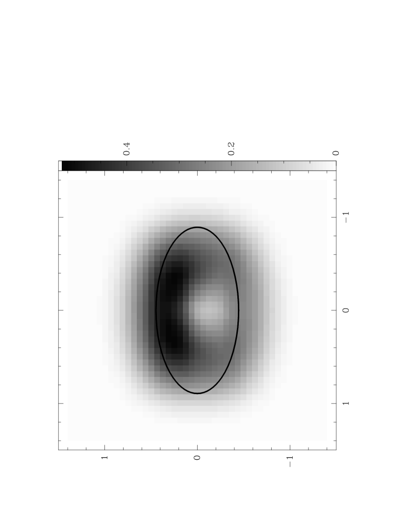
Figure 4: Gray scale map of the integrated intensity of C${}^{17}$O($3\rightarrow 2$) for a disk with $i=60^{\circ}$, and thermal line profiles, convolved with a beam of 0$\farcs$4.

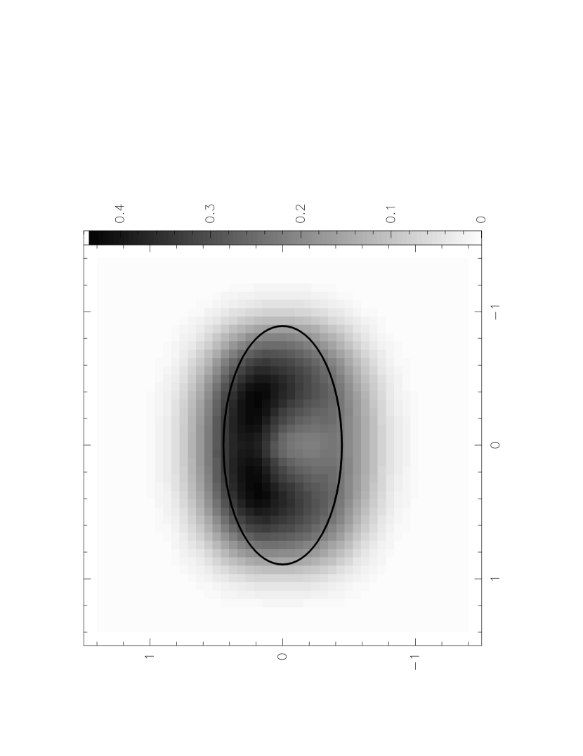
Figure 5: Same as Fig. 4, but for C${}^{17}$O($2\rightarrow 1$) line emission.

Detailed maps and spectra obtained from our calculations in the particular case of the C${}^{17}$O($3\rightarrow 2$) and ($2\rightarrow 1$) transitions are shown in Figures 2, 3, 4, 5, 6, 7, 8, and 9. These results also correspond to the HL Tau structure model described in §2, and they are convolved to a resolution of 0$\farcs$4.

The channel maps in Figs. 2 and 3 are plotted with the projected major axis of the disk lying along a line of constant declination. With the assumed inclination angle of 60°, the southern half of the disk is closer to the observer than the northern one. The central star is located at position (0,0).

In these maps, we can see several characteristics that eventually can be tested observationally. First, we see a clear north-south asymmetry; the areas of the disks that are farther away from the observer show a more intense line emission than those that are closer. This is an expected behavior for optically thick lines in a disk of finite thickness. In these cases, for the same projected distance from the star, the lines of sight intersect the disk surface closer to the star (thus tracing warmer gas) in those areas that are inclined farther away from the observer. This effect can also be seen in the integrated line intensity (Fig. 4). If this asymmetry is actually observed, it could be compared with observations of jets and outflows, to see if they are consistent with each other. For instance, redshifted lobes of outflows should be projected in the same direction as the part of the disk closest to us, assuming that disks and outflows are perpendicular. The east-west asymmetry that can be seen at $v=0$ km s${}^{-1}$(Fig. 2) is due to the asymmetric hyperfine structure of the C${}^{17}$O lines.

We can also see in Fig. 2, that the peak emission for the lowest velocities tend to trace the outer edge of the disk. One of the reasons for the molecular line flux to trace the outer parts of the disk (as already pointed out by Sargent & Beckwith 1991) is that the effective area emitting at a definite velocity within the telescope beam increases with distance from the star, and more steeply than an eventual decrease of brightness temperature with distance. This effect is also the reason of the double peaked profiles that is typical of line emission from rotating structures.

This geometrical effect is further reinforced by the opacity of the dust continuum emission. If the continuum optical depth tends to infinity, the brightness temperature for both line+continuum and continuum alone will be equal to the kinetic temperature at the disk surface. Therefore, there would be no contrast between the line and the continuum emission, and the line would be undetectable. Thus, the effect of high continuum opacities is to effectively reduce the brightness temperature of the line (after subtracting the continuum), i.e., to reduce the contrast between line and continuum. This decrease of brightness temperature is important as we approach the parts of the disk closer to the star (with higher densities, and therefore with higher continuum opacities), but not in the outer parts, where the continuum is usually optically thin. Moreover, in a real disk with high (but not infinity) continuum optical depth close to the star, the opacity is higher at frequencies with line emission (due to the contribution of line+continuum) than at those with continuum emission alone. Therefore, the continuum emission gets optically thick deeper into the disk than the line+continuum emission. As the temperature increases as we move vertically towards the disk midplane, the molecular lines could be seen in absorption in these high opacity regions (see Figs. 6, 7).

One of the results of this opacity effect is that the integrated intensity map (Figs. 4 and 5) shows the appearance of a ring, with lower emission at the center. When detecting such a ring-like structure, one could be tempted to wrongly conclude that the lower emission corresponds to a lower amount of gas, as in a toroidal gas distribution. This result illustrates that it is important to properly consider the contribution of the continuum emission from dust in these calculations of line emission, a contribution that sometimes is ignored.

4.3 Position-Velocity Diagrams

Figs. 8 and 9 show position-velocity diagrams along lines with constant declination and right ascension, respectively. Superimposed to those diagrams there are lines that mark the corresponding mid-plane Keplerian velocity at each position, taking into account the distance from the star and the inclination angle of the disk. We see that the emission peaks in the cut along the major axis of the projected disk (Fig. 8, top left) would be enough to give us an estimate of the mass of the central star, provided that we have independently determined the inclination angle of the disk. In fact, molecular line observations can help in this determination, although it is not straightforward (see §5.1). The fit of the other position-velocity diagrams to the Keplerian lines is not as good as for the cut along the major axis, due to the finite angular resolution ($0\farcs 4$). We could try a more refined fit of the position-velocity diagram to the lines of Keplerian velocities, by looking whether the emission maxima at each velocity are relatively close to the Keplerian lines (see, e.g., Sargent & Beckwith 1991, for the large-scale structure in HL Tau). However, as we can see by taking a close look at Fig. 8 (top left), those emission maxima are close to the Keplerian expectation at high relative velocities (with absolute value higher than 2 km s${}^{-1}$ in this particular case), but depart significantly from it at the lowest velocities, for which the emission maxima are located closer to the star than in the corresponding Keplerian line.

5 Effects of changes in physical parameters

5.1 Inclination angle

An obvious question to ask is what qualitative and quantitative effect would be observable if a disk with the physical structure of that of HL Tau is located to an inclination angle with respect to us different from the $60^{\circ}$ assumed here, and obtained from the continuum observations in HL Tau. To illustrate these effects, we show in Figs. 10 and 11 the results of our calculations with an inclination angle of $30^{\circ}$, of the C${}^{17}$O($3\rightarrow 2$) transition.

In quantitative terms, the maximum intensity for $i=30^{\circ}$ is 325 mJy beam${}^{-1}$ (with a beam of 0$\farcs$4), which is 25% higher than the maximum intensity for the same transition in the disk at $i=60^{\circ}$. Qualitatively, an important difference can be seen in the spectra (Fig 11, to be compared with Fig 6). The double peak in the central spectrum is much less prominent for $i=30\arcdeg$, while for $i=60\arcdeg$ there was a significant self-absorption. Therefore, the combination of lower radial velocities and lower optical depth in less inclined disks makes this central spectral feature very sensitive to the value of the inclination angle. It would be difficult to use this absorption feature alone to estimate the inclination angle of the disk, because a similar self-absorption can be produced by strong vertical temperature gradients. However, it can be an important piece of information that, together with other observational evidences, can be used to self-consistently obtain the disk structure and the inclination angle, in a similar way as explained in sec. 2.

The observed aspect ratio of the integrated intensity (Fig. 4) is somewhat correlated with the inclination angle, but it does not directly indicate its value. If we measure the distance between integrated intensity peaks on each side of the central star, for both the major and minor axes, to obtain this aspect ratio, it would give an apparent inclination angle of $\sim 30^{\circ}$ for $i=60^{\circ}$, and $\sim 20^{\circ}$ for $i=30^{\circ}$. Therefore, the derivation of the inclination angle from geometrical considerations must be made with care.

We also note that the maxima of emission at each velocity (see Fig. 10) does not follow the outer radius of the disk, as it did for the disk at $i=60\arcdeg$

5.2 Turbulent velocity

In this section, we show how the above calculations change when there is a turbulent velocity field, in addition to thermal and rotational motions of the gas. To check for the maximum possible effect that the inclusion of turbulence will have on the line spectra, we use an upper limit to the turbulence velocity, which we assume equal to the thermal velocity (see §3.1).

The turbulent velocity modifies the profile given by Eq. (11). If we assume a Gaussian distribution for the turbulent velocity field, the resulting profile will also be Gaussian, and can be written as

$$\Psi(v)=\frac{c}{\nu}\left({1\over\zeta_{\circ}\pi^{1/2}}\right)\exp\left[-\frac{(v-v_{\circ})^{2}}{\zeta_{\circ}^{2}}\right]\;,$$ (13)

where

$$\zeta_{\circ}^{2}={2kT\over m_{\rm mol}}+\zeta_{T}^{2}$$ (14)

and $\zeta_{T}$ is the turbulent velocity dispersion we have assumed equal to the thermal velocity dispersion of a particle with a mass equal to the mean molecular mass $m_{o}$, i.e., $\zeta_{T}^{2}={2kT\over m_{o}}$ (see §3.1).

A comparison between Figs. 2 and 12 shows that the line intensity increases (roughly by a factor 3, for the turbulent velocity adopted in our calculations) if a turbulent velocity is included in the line profile calculation. The main reason of this enhancement of the emission is that the line opacity decreases when the velocity of the emitting molecules increases (see Eqs. (9) and (13)). Thus, the “turbulent lines” are dominated by emission from a deeper, hotter region than those involved in the intensity of a “pure thermal line”.

From an observational point of view, this enhancement of the intensity of the lines when turbulence is considered, will obviously make the detection of these lines easier. Thus, the conclusions one can draw from Table 2 in terms of detectability should be considered as the less favorable case, since that line intensities in a non-turbulent scenario are lower limits to the lines intensities with some turbulent contribution.

The mean increase in linewidth is only of $\sim 0.4$ km s${}^{-1}$ when applying a turbulent component at sound speed. This means that the line profile is dominated by rotational motion, which makes it difficult to determine the turbulent velocity from line profiles. Such a determination will require a high spectral resolution and high sensitivity, but it may be necessary if we want to derive physical characteristics of disks from line emission. Since turbulence causes strongest lines, it could be confused by the effect that a different density and/or temperature structure may cause.

5.3 Generalization to other sources

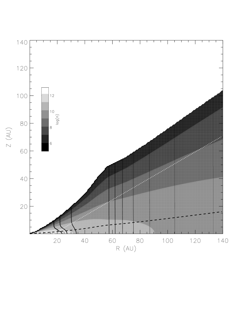
Figure 1: Map of temperature (Solid contour lines) and number density of hydrogen molecules (greyscale) for a model of an accretion disk irradiated by an infalling envelope. The disk has $\dot{M}=10^{-6}\ \rm M_{\odot}\,yr^{-1}$ and $\alpha=0.04$, and surrounds a star with $M_{*}=0.5\ \rm M_{\odot}$ and $R_{*}=3\ \rm R_{\odot}$. The envelope is flat, with $\dot{M}_{env}=4\times 10^{-6}\ \rm M_{\odot}\,yr^{-1}$ (see DCH and HCB for details). The increment step for temperature contours is 5 K and the lowest temperature plotted (the rightmost one) is 25 K, with thicker contours indicating larger temperature values. The gas scale height is shown as a heavy dark dashed line, and the line of sight, assuming an inclination angle $i=60\ ^{\circ}$ for the disk axis, is plotted with a dotted white line.

In this paper we have used a disk structure that is consistent with observational data for the relatively well constrained disk of HL Tau. An important issue is whether our conclusion that such a disk will be detectable with millimeter interferometers is of general applicability to other sources, with different disk structures in density and temperature. This is not an easy question to address, since to derive a realistic disk structure will require a wealth of data that, at present, is probably only available for HL Tau (see sec. 2). However, we can obtain some answers by checking how changes in temperature and density affect a possible detectability of molecular line emission. The range of values we have explored goes from $T_{\circ}/5$ to $5T_{\circ}$ and from $n_{\circ}/100$ to $100n_{\circ}$, where $T_{\circ}$ and $n_{\circ}$ are the temperature and volume density of the original HL Tau model (Fig. 1). The resulting maps are very similar morphologically to the ones obtained above for the HL Tau model. Spectral signatures and diagnosis mentioned in the previous sections (e.g., asymmetry of the line emission, enhancement of line emission towards the edges, tracing of Keplerian velocities, changes of central self-absorption as a function of inclination angle, emission enhancement with turbulent motions) are of general applicability in these parameter ranges, which include typical Class I sources (see below).

The main result is that the peak intensity of the maps is much more sensitive to temperature than to density variations. For instance, for the C${}^{17}$O(J$=3\rightarrow 2$) lines, the relation of intensity with temperature is linear, while the volume density dependence is as shown in Fig. 13, with variations of less than a factor of 5 over 4 orders of magnitudes in density. The conclusion in terms of detectability is that one should tend to observe the hottest disk sources to ensure an easier detection.

We can further focus on the detectability of disks in Class I sources in general. In the context of the model of an accretion disk irradiated by an infalling envelope, the density scales as $\dot{M}/\alpha$ (c.f. §2) and the temperature is controlled by the emergent flux from the envelope. The last one depends on the input luminosity provided by the central star and the inner disk (i.e., $L_{*}$ and $L_{acc}\propto\dot{M}$). Taking the envelope irradiation flux proportional to the input luminosity (Calvet, private communication), the irradiation temperature is $T_{irr}\propto L^{1/4}$, which is equal to the disk photospheric temperature for $R\gtrsim 1\ \rm AU$ (DCH). In the case of HL Tau, the input luminosity is $L=5\ \rm L_{\odot}$. However, the median luminosity of Class I sources is $\sim 1\ \rm L_{\odot}$ (e.g., Kenyon & Hartmann 1995). Thus, the disk of a typical Class I source would have a photospheric temperature 0.7 times the temperature we calculate for the HL Tau model. On the other hand, Muzerolle, Hartmann & Calvet (1998) estimate that typical Class I sources have mass accretion rates similar to classical T Tauri stars, $\dot{M}\sim 10^{-8}-10^{-7}\ \rm M_{\odot}\,yr^{-1}$, with a median $\dot{M}=10^{-7}\ \rm M_{\odot}\,yr^{-1}$ (Calvet, Hartmann & Strom 1999). The density of such a disk is a factor of $100-10$ lower than the density of the HL Tau disk model, assuming the same viscosity parameter $\alpha$. Combining the dependence of flux on both density (as shown in Fig. 13) and temperature (linear), and using $n=n_{\circ}/100$ and $T=0.7T_{\circ}$, we estimate that the molecular lines of a typical Class I source would have at worst 0.18 times the intensity we have calculated for the HL Tau model. Thus, the worst case implies that the C${}^{17}$O(J$=3\rightarrow 2$) lines of Class I sources would be detectable in a reasonable observing time with the MMA, but are probably not detectable using SMA.

5.4 Molecular abundances

An issue of concern is the possibility of molecular depletion within the disk, since one would think that lower molecular abundances will make molecular lines more difficult to detect. In the calculations presented in this paper, we have used a constant abundance, which in most cases is the interstellar one (for CS we assumed an abundance given in Blake et al. (1992) for the disk in HL Tau, lower than the interstellar one). Theoretical models of the evolution of molecular abundances in protoplanetary disks predict depletion of CO from the gas phase for temperatures $T\ <$ 20 K (Aikawa et al. 1996 ) and of NH${}_{3}$, for $T\ <$ 80 K (Aikawa et al. 1997). The application of these results to the HL Tau model is not straightforward, since there are differences between the physical conditions of their disk model and ours. However, since the most relevant disk property in determining molecular abundances is the temperature (Aikawa et al. 1996), and for $R>10$ AU our model has a radial distribution of photospheric temperature similar to the model used by Aikawa et al. (1996, 1997) we adopt some of their results in this discussion. The HL Tau disk model (with $R_{d}=125$ AU) has a temperature higher than the critical temperature for freezing $\sim 20$ K (reached at $R\simeq 200$ AU, in the disk model of Aikawa et al. 1996, 1997). On the other hand, the timescale for transforming CO into CO${}_{2}$ ice at $T\simeq 30$ K is larger than $\sim 1$ Myr (Aikawa et al. 1996), and the viscous timescale of our disk model is $\sim 0.1$ Myr (DCH). Therefore, depletion is probably not significant for CO lines (which are our best candidates for detection) in the conditions of our HL Tau model.

For typical Class I sources, with temperatures 0.7 times that of HL Tau, we have checked that the maximum intensity of C${}^{17}$O lines is the same with and without considering depletion, for different beam sizes (0$\farcs$4, 0$\farcs$6, 0$\farcs$8). Therefore, depletion does not seem to be important regarding line detectability in typical Class I sources. For even colder sources, CO depletion could, in principle, affect detectability if a significant fraction of the disk is below the critical temperature of 20 K.

Depletion of NH${}_{3}$ from the gas phase at $T<80$ K ($R\gtrsim$ 20 AU) will probably decrease the intensity of the ammonia lines with respect to our calculations, confirming our conclusion that these lines are not good candidates for detecting protoplanetary disks.

Blake et al. (1992) find that CS is depleted in the disk of HL Tau respect to the molecular cloud, and we have used the lowest abundance they have estimated (see Table 1) for calculating the CS and C${}^{34}$S lines. However, Blake et al. (1992) observations do not resolve the inner $\sim$ 100 AU region of HL Tau, and we could be underestimating the abundance of CS. Thus, we calculate the maximum intensity of the line CS(J$=1\rightarrow 0$) assuming an abundance $X_{mol}=5\times 10^{-9}$ (Aikawa et al. 1996), i.e., a factor of 25 larger than the abundance quoted in Table 1. The maximum intensity is $F_{\nu}=9.6$ mJy beam${}^{-1}$, for a beam size of $0\farcs 4$, which is still too low to be detected in a reasonable observing time given the sensitivity of the VLA.

In any case, the study of molecular abundances in disks will certainly benefit from accurate observational data, which can be obtained with the type of observations we are trying to reproduce. The results of our model can also help to interpret observational results in terms of abundance changes.

6 Conclusions

In this work we model the expected line emission from a protoplanetary disk irradiated by an infalling envelope, when observed with subarcsecond resolution. We adopt a model for the disk structure consistent with the available observational constraints for HL Tau. Our main conclusion is that the detection of molecular lines at subarcsecond resolution will be within reach of the projected millimeter and submillimeter interferometers (e.g., MMA, SMA). In particular, an instrument like the MMA has enough sensitivity to provide important data to constrain disks models.

We suggest that the lines C${}^{17}$O($2\rightarrow 1$) and ($3\rightarrow 2$), at $\lambda=$1.335 and 0.89 mm, respectively, are good candidates for detecting disk lines at subarcsecond resolution, because the infalling envelope is probably optically thin at the corresponding wavelengths (CHKW). Also, these lines are more intense than others from more abundant species (e.g., C${}^{18}$O) due to opacity effects combined with the temperature gradients in the disk.

There is a clear asymmetry in the line intensity, with more intense emission in the disk area farther away from the observer. This can be directly used to compare the geometrical relationship between disks and outflows. A decrease of intensity towards the center of the disk is also evident.

The emission peaks in position-velocity diagrams lie on the lines that trace mid-plane Keplerian velocities. This can be used to determine the stellar mass, but only if and independent estimate of the inclination angle of the disk can be obtained.

Some changes in physical properties are correlated with changes in line intensity and spectral shape:

• Line intensity decrease as the inclination angle increases.

• For larger inclination angles, a central absorption feature in the spectra becomes deeper.

• Increasing the turbulent velocity results in brighter lines, but only in a moderate enhancement of linewidth.

• The line intensity scales linearly with disk temperature, but is less sensitive to density changes.

Going the opposite way, i.e., obtaining physical properties of disks from line shape and intensity is not straightforward, since a similar observational characteristic can be explained by several alternative physical changes. However, the information provided by molecular line observations can eventually be used, together with continuum data, to obtain a self-consistent model that could explain all observational evidence.

Expected changes in molecular abundances do not affect our results regarding the detectability of molecular lines from disks, at least for typical Class I sources.

We plan to extend this study to models of disks in a later state of evolution, not surrounded by an infalling envelope but irradiated by the central star. A detailed calculation of how the line properties depend on disks parameters could be a useful disk diagnostic tool.

Appendix A Some details on the integration process

A.1 Projected Velocities

Fig. 14 shows the geometry of the problem, and how to calculate Doppler shifts of the gas. A gas element at radius $r$ from the central star rotates with a Keplerian velocity

$$v=\sqrt{\frac{GM_{*}}{r}}\;.$$ (A1)

At a particular point on its orbit, defined by angle $\theta$, the projected velocity along the line of sight, for an inclination angle $i$, is

$$v_{\circ}=\sqrt{\frac{GM_{*}}{r}}\cos\theta\sin i\;.$$ (A2)

A.2 Grid

To integrate the transfer equation, we divided the disk into a grid of cells. The transfer equation is then solved for a line of sight going through the center of each cell. To create this grid, we first calculate the lines on the disk midplane with the same projected velocity, which are of the form

$$r=\frac{GM_{*}}{v^{2}_{\circ}}\cos^{2}\theta\sin^{2}i\;.$$ (A3)

These lines are shown in Fig. 15a.

Up to a radius of 50 AU, the grid is defined so that the borders of the cells are these isovelocity lines and their perpendicular lines (of the form $r=A\sqrt{(\sin\theta)}$, where $A$ is a constant), so that all cells have the same velocity resolution, that we choose to be lower that the thermal velocity width of the gas. This grid avoids a possible overestimate of the fluxes in the inner disk at the velocities we sample. This overestimate would happen if cells include a range of projected velocities larger than the thermal velocity of the gas. An example of the grid we chose is shown in Fig. 15b. For radii larger than 50 AU, the cells on this grid have a large area. This makes the sampling of temperature and density poorer on those areas and therefore we chose a Cartesian grid, with smaller cells than those corresponding to the grid shown, thus keeping the velocity range covered by each cell below the thermal velocity width of the gas.

A.3 Coordinate Systems

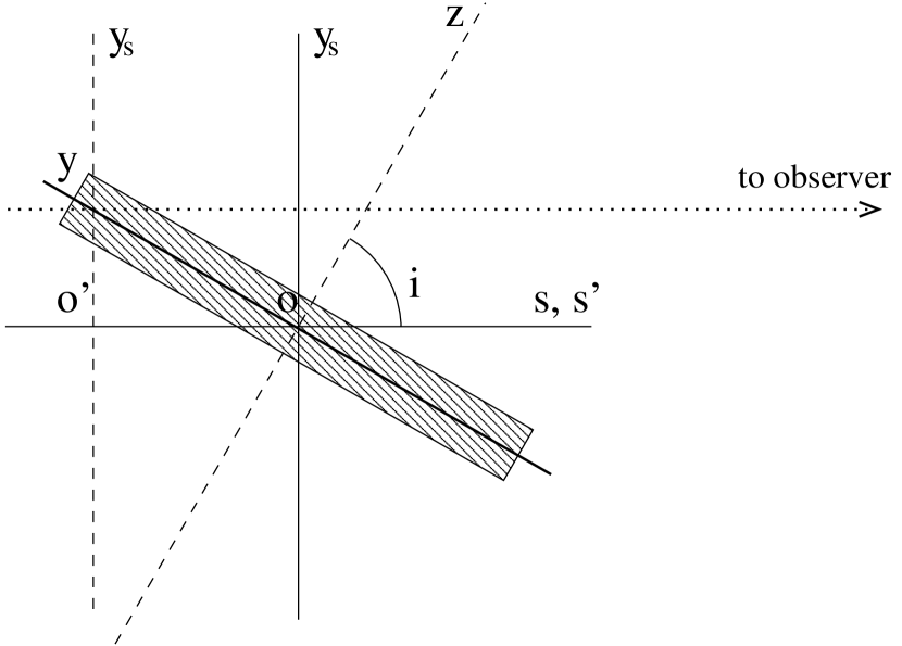
Figure 16: Geometry of the coordinate system used in the integration of the transfer equation (see text).

In this section, we define the coordinate system used in the integration of the transfer equation. We found this coordinate system to be convenient for an easy transformation of all the equations. Fig. 16 illustrates the coordinate systems mentioned in this section.

We first consider the “disk” coordinate system $(x,y,z)$, centered on $O$ (the position of the central star). The axes $x$ and $y$ are on the disk plane. Axis $z$ represents the height from the disk midplane. Equations for temperature and density of the disk are given naturally on this coordinate system.

We can also consider the “sky” coordinate system $(x_{s},y_{s},s)$, centered on $O$. Axis $x_{s}$ coincides with $x$. Axes $x_{s}$ and $y_{s}$ are on the plane of the sky. Axis $s$ is along the line of sight.

The system we use for the integration (“integration” coordinate system) is $(x_{s},y_{s},s^{\prime})$, centered on $O^{\prime}$. It is just a translation of the “sky” system along axis $s$, so that coordinates on axis $s^{\prime}$ equal zero when the line of sight intersects the disk midplane. Note that there is actually a different coordinate system for each line of sight, i.e., for every point on the sky where we integrate the transfer equation, we use a different coordinate system.

The transformation between the “disk” and “integration” coordinate systems is then

$$y=\frac{y_{s}}{\cos i}-s^{\prime}\sin i$$ (A4)

$$z=s^{\prime}\cos i\;.$$ (A5)

Equations that define the physical characteristics of the disk are then transformed into the “integration” coordinate system. Integration of the transfer equation is performed in two parts, from $s^{\prime}=+\infty$ to 0, and from 0 to $-\infty$, to properly sample the disk midplane.

Figure 2: Channel maps of C${}^{17}$O($3\rightarrow 2$) line emission, for a disk with $i=60^{\circ}$, and thermal line profiles, convolved with a beam of 0$\farcs$4. The lowest positive contour and the increment step are 20 mJy beam${}^{-1}$. The velocity with respect to the rest system of the central star is shown at the top left corner of each panel. The thick ellipse corresponds to the disk maximum radius projected on the plane of the sky.

Figure 3: Same as Fig. 2, but for C${}^{17}$O($2\rightarrow 1$) line emission.

Figure 6: Spectra of the C${}^{17}$O($3\rightarrow 2$) line emission at selected positions, for a disk with $i=60^{\circ}$, and thermal line profiles, convolved with a beam of 0$\farcs$4. Position offsets, in arcseconds, with respect to the central star are indicated at the top right corner of each panel. Solid and dashed lines correspond to the spectra at positive and negative declination offsets, respectively.

Figure 7: Same as Fig. 6, but for C${}^{17}$O($2\rightarrow 1$) line emission.

Figure 8: Position-velocity diagrams of C${}^{17}$O($3\rightarrow 2$) emission, along lines of constant declination (indicated at the top right corner of each panel), i.e., parallel to the mayor axis of the projected disk, assuming $i=60^{\circ}$ and thermal line profiles, and convolved with a beam of 0$\farcs$4. The lowest positive contour and the increment step are 20 mJy. Thin solid lines correspond to Keplerian laws, for different values for the mass of the central star, $M_{*}=0.25,\ 0.5,$ and $1\ \rm M_{\odot}$. The disk model constructed for HL Tau, assumes that the central star has $M_{*}=0.5\ \rm M_{\odot}$.

Figure 9: Position-velocity diagrams of C${}^{17}$O($3\rightarrow 2$) emission, along lines of constant right ascension (indicated at the top right corner of each panel), i.e., parallel to the minor axis of the projected disk, assuming $i=60^{\circ}$ and thermal line profiles, and convolved with a beam of 0$\farcs$4. The lowest positive contour and the increment step are 20 mJy beam${}^{-1}$. Thin solid lines correspond to Keplerian laws at the disk midplane, for different values for the mass of the central star, $M_{*}=0.25,\ 0.5,$ and $1\ \rm M_{\odot}$. The disk model constructed for HL Tau, assumes that the central star has $M_{*}=0.5\ \rm M_{\odot}$.

Figure 10: Same as Fig. 2, but for an inclination angle $i=30^{\circ}$.

Figure 11: Same as Fig. 6, but for $i=30^{\circ}$.

Figure 12: Channel maps of C${}^{17}$O($3\rightarrow 2$) line emission, for a disk with $i=60^{\circ}$, including a turbulent component for the line profile and convolved with a beam of 0$\farcs$4. The lowest positive contour and the increment step are 20 mJy beam${}^{-1}$. The velocity with respect to the rest system of the central star is shown at the top left corner of each panel. The thick ellipse corresponds to the disk maximum radius projected on the plane of the sky.

Figure 13: Peak flux of the C${}^{17}$O($3\rightarrow 2$) line as a function of disk density, for $v=1$ km s${}^{-1}$. The x-axis is the logarithm of the ratio between the density and the original density model ($n_{\circ}$) used for HL Tau.

Figure 14: Geometry of the disk and projections of the Keplerian velocity of the gas, with respect to the observer. The disk seen face-on, is shown at the left. At the right, the disk is located edge-on, along the direction of vector $v^{\prime}$. The projected velocity along the line of sight is $v_{\circ}$.

Figure 15: (a) Lines of equal projected velocities in the NW quadrant of a disk with inclination angle $i=60^{\circ}$. The interval between adjacent lines is 0.1 km s${}^{-1}$. The thick curve is disk outer radius. (b) Example of the type of grid used in the integration. It is formed by the isovelocity lines shown in (a), and their perpendicular lines.

Table 1: Molecular Parameters

Molecule	Dipole Moment	$X_{\rm mol}$	References
	(Debye)
C${}^{18}$O	$0.112$	$2.0\times 10^{-7}$	1, 2
C${}^{17}$O	$0.112$	$5.0\times 10^{-8}$	1, 3
CS	$1.957$	$2.0\times 10^{-10}$	4, 5
C${}^{34}$S	$1.957$	$8.8\times 10^{-12}$	4
NH${}_{3}$	$1.468$	$1.0\times 10^{-8}$	6, 7

References. — (1) Rohlfs 1986, (2) Frerking et al.  1982, (3) White & Sandell 1995, (4) Winnewisser & Cook 1968, (5) Blake et al.  1992, (6) Townes & Schawlow 1975, (7) Herbst & Klemperer 1973

Table 2: Line Intensities and Telescope Sensitivities for 0$\farcs$4 Resolution Observations

Line	$\nu_{\circ}$	$F_{\nu}$ (0$\farcs$4)	Telescope	Sensitivity $(1\sigma)$
	(GHz)	(mJy beam${}^{-1}$)		(mJy beam${}^{-1}$)
C${}^{18}$O$(2\rightarrow 1)$	219.5604000	120	MMA	0.5
			SMA	30
C${}^{18}$O$(3\rightarrow 2)$	392.3305722	220	MMA	0.7
			SMA	80
C${}^{17}$O$(2\rightarrow 1)$	224.7143680	140	MMA	0.5
			SMA	30
C${}^{17}$O$(3\rightarrow 2)$	337.0611000	260	MMA	0.7
			SMA	80
CS$(1\rightarrow 0)$	48.9909780	5.9	VLA (13)	3.0
			VLA (27)	1.3
CS$(2\rightarrow 1)$	97.9809500	28	MMA	0.4
CS$(3\rightarrow 2)$	146.9690330	58	MMA	0.4
C${}^{34}$S$(1\rightarrow 0)$	48.2069150	0.6	VLA (27)	1.3
C${}^{34}$S$(2\rightarrow 1)$	96.4129400	7.0	MMA	0.4
C${}^{34}$S$(3\rightarrow 2)$	144.6171090	25	MMA	0.4
C${}^{34}$S$(5\rightarrow 4)$	241.0161940	62	MMA	0.5
NH${}_{3}$(1,1)	23.6944955	2.4	VLA	2.0
NH${}_{3}$(2.2)	23.7226333	2.5	VLA	2.0
NH${}_{3}$(3.3)	23.8701292	2.5	VLA	2.0
NH${}_{3}$(4,4)	24.1394163	2.2	VLA	2.0

Note. — Sensitivities calculated for 10 h of observing time and 1 km s${}^{-1}$ velocity resolution, for a disk with $i=60^{\circ}$. MMA sensitivity information from Rupen (1997), for an array of 40$\times$8m antennas; SMA, from Masson et al. (1992); VLA from its WWW page as of 1998 March 6

References

- (1)
- (2) Adams, F. C., Shu, F. H., & Lada, C. J. 1988, ApJ, 326, 865
- (3) Aikawa, Y., Miyama, S. M., Nakano, T., & Umebayashi, T. 1996, ApJ, 467, 684
- (4) Aikawa, Y., Umebayashi, T., Nakano, T., & Miyama, S. M. 1997, ApJ, 486, 51
- (5) Balbus, S. A., & Hawley, J. F. 1991, ApJ, 376, 214
- (6) Beckwith, S. V. W., Koresko, C. D., Sargent, A. I. 1989, ApJ, 343, 393
- (7) Beckwith, S. V. W., Sargent, A. I., Chini, R. S., & Guesten, R. 1990, AJ, 99, 1024
- (8) Beckwith, S. V. W.,& Sargent, A. I. 1991, ApJ, 381, 250
- (9) Beckwith, S. V. W., & Sargent, A. I. 1993, ApJ, 402, 280
- (10) Bertout, C., Basri, G. & Bouvier, J. 1988, ApJ, 330, 350
- (11) Blake, G. A., Van Dishoeck, E. F., & Sargent, A. I. 1992, ApJ, L99
- (12) Burrows, C. J., et al. 1996, ApJ, 473, 437
- (13) Cabrit, S., Guilloteau, S., Andre, P., Bertout, C., Montmerle, T., & Schuster, K. 1996, A&A, 305, 527
- (14) Calvet, N., Patiño, A., Magris, G., & D’Alessio, P. 1991, ApJ, 380, 617
- (15) Calvet, N., Hartmann, L., Kenyon, S., & Whitney, B. 1994, ApJ, 434, 330 (CHKW)
- (16) Calvet, N., Hartmann, L., & Strom, S.E. 1999, In Protostars and Planets IV, ed. V. Mannings, A. P. Boss & S. S. Russell (Tucson: University of Arizona Press), in press
- (17) Carr, J. S., Tokunaga, A. T., Najita, J., Shu, F. H., & Glassgold, A. E. 1993, ApJ, 411, 37
- (18) D’Alessio, P., Calvet, N., & Hartmann, L. 1997, ApJ, 474, 397 (DCH)
- (19) Draine, B. T., & Lee, H. M. 1984, ApJ, 285,89
- (20) Dubrulle, B., 1992, A&A, 266, 592
- (21) Dutrey, A., Guilloteau, S., & Simon, M. 1994, A&A, 286, 149
- (22) Frank, J., King, A.R., & Raine, D. J. 1992, in Accretion power in Astrophysics, (Cambridge:University Press), 72
- (23) Frerking, M. A., Langer, W. D., & Wilson, R. W. 1982, ApJ, 262, 590
- (24) Galli, D., & Shu, F. H. 1993a, ApJ, 417, 220
- (25) Galli, D., & Shu, F. H. 1993b, ApJ, 417, 243
- (26) Gómez, J. F., & D’Alessio, P. 1995, in Disks, Outflows and Star Formation, ed. S. Lizano & J. M. Torrelles, RevMexAASC, 1, 339
- (27) Gómez, J. F., Torrelles, J. M., Ho, P. T. P., Rodríguez, L. F., & Cantó, J. 1993, ApJ, 414, 333
- (28) Grasdalen, G. L., Sloan, G., Stout, N., Strom, S. E., & Welty, A. D. 1989, ApJ, 339, 37
- (29) Hartmann, L., Boss, A., Calvet, N., & Whitney, B. 1994, ApJ, 430, 49
- (30) Hartmann, L., Calvet, N., & Boss, A. 1996, ApJ, 464, 387 (HCB)
- (31) Hartmann, L., & Kenyon, S. J. 1985, ApJ, 299, 462
- (32) Hartmann, L., & Kenyon, S. J. 1987a, ApJ, 312, 243
- (33) Hartmann, L., & Kenyon, S. J. 1987b, ApJ, 322, 393
- (34) Hawley, J. F., Gammie, C. F., & Balbus, S. A. 1995, ApJ, 440, 742
- (35) Hayashi, M., Ohashi, N., & Miyama, S. 1993, ApJ, 418,L71
- (36) Herbst, E., & Klemperer, W., 1973, ApJ, 185, 505
- (37) Keene, J., & Masson, C.R. 1990, ApJ, 355, 635
- (38) Kenyon, S. J., Hartmann, L., & Hewett, R. 1988, ApJ, 325, 231
- (39) Koerner, D. W., Sargent, A. I., & Beckwith, S. V. W. 1993, ApJ, 408, 93
- (40) Lay, O. P, Carlstrom, J. E., Hill, R. E., & Phillps, T. G. 1994, ApJ, 434, L75
- (41) Lay, O. P., Carlstrom, J. E. & Hill, R. E. 1997, ApJ, 489, 917
- (42) Masson, C., Bloemhof, E., Blundell, R., Bruckman, W., Ho, P., Keto, E., Levine, M., Raffin, P., Reid, M., Wolfire, M. 1992, Design Study for the Submillimeter Interferometer Array of the Smithsonian Astrophysical Observatory
- (43) McCaughrean, M. J., & O’Dell, C. R., 1996, AJ, 111, 1977
- (44) Morfill, G. E. 1989, in Low Mass Star Formation and Pre-Main Sequence Objects, ed. B. Reipurth (Garching:ESO), 191
- (45) Mundy, L. G., Looney, L. W., Erickson, W., Grossman, A., Welch, W. J., Froster, J. R., Wright, M. C. H., Plambeck, R. L., Lugten, J., & Thornton, D. D. 1996, ApJ, 464, 169
- (46) Muzerolle, J., Hartmann, L., & Calvet, N. 1998, AJ, 116, 2965
- (47) Najita, J., Carr, J. S., Glassgold, A. E., Shu, F. H., Tokunaga, A. T. 1996, ApJ, 462, 919
- (48) Najita, J., Edwards, S., Basri, G., & Carr, J. 1999, In Protostars and Planets IV, ed. V. Mannings, A. P. Boss & S. S. Russell (Tucson: University of Arizona Press), in press
- (49) O’Dell, C. R., Wen, Z., & Hu, X. 1993, ApJ, 410, 696
- (50) Omodaka, T., Kitamura, Y., & Kawazoe, E. 1992, ApJ, 396, 87
- (51) Press, W. H., Flannery, B. P., Teukolsky, S. A., & Vetterling, W. T. 1992, in Numerical Recipes in Fortran, (Cambridge:University Press)
- (52) Rodríguez, L. F., Cantó, J., Torrelles, J. M., & Ho, P. T. P. 1986, ApJ, 301, L25
- (53) Rodríguez, L. F., Cantó, J., Torrelles, J. M., Gómez, J. F., & Ho, P. T. P. 1992, ApJ, 393, L29
- (54) Rodríguez, L. F., Cantó, J., Torrelles, J. M., Gómez, J. F., Anglada, G., & Ho, P. T. P. 1994, ApJ, 427, L103
- (55) Rohlfs, K. 1986, In Tools of Radio Astronomy (Heidelberg:Springer)
- (56) Rupen, M. P. 1997, MMA Memo 192
- (57) Sargent, A. I., & Beckwith, S. V. W. 1991, ApJ, 382, 31
- (58) Shakura, N. I., & Sunyaev, R. A. 1973, A&A, 24, 337
- (59) Shakura, N. I., Sunyaev, R. A., & Zilitinkevich, S. S. 1978, A&A, 62, 179
- (60) Stapelfeldt, K. R., et al. 1995, ApJ, 449, 888
- (61) Stauffer, J. R., Prosser, C. F., Hartmann, L., & McCaughrean, M. J. 1994, AJ, 108, 137
- (62) Terebey, S., Shu, F. H., & Cassen, P. 1984, ApJ, 286, 529
- (63) Townes, C. H., & Schawlow, A. L. 1975, In Microwave Spectroscopy (New York:Dover)
- (64) White, G. J., & Sandell, G. 1995, A&A, 299,179
- (65) Wilner, D. J., Ho, P. T. P., & Rodríguez, L. F. 1996, ApJ, 470, 117
- (66) Winnewisser, G., & Cook, R. L. 1968, J. Mol. Spect., 28, 266
- (67) Zhan, J. 1991, Ph. D. Thesis, Rice University
- (68)