Cosmic Glows

Abstract

This is the obligatory Cosmic Microwave Background review. I discuss the current status of CMB anisotropies, together with some points on the related topic of the Far-Infrared Background. We have already learned a number of important things from CMB anisotropies. Models which are in good shape have: approximately flat geometry; cold dark-matter, plus something like a cosmological constant; roughly scale invariant adiabatic fluctuations; and close to Gaussian statistics. The constraints from the CMB are beginning to be comparable to those from other cosmological measurements. With a wealth of new data coming in, it is expected that CMB anisotropies will soon provide the most stringent limits on a combination of fundamental cosmological parameters.

Keywords: CMB – FIB – Monty Python

1 ‘Always Look on the Bright Side of Life’

Much of the matter in the Universe is in a form which is not very luminous. There is additional evidence that majority of the cosmological density is contained in some even more mysterious Dark Energy. However, we learn most about the Universe by studying the properties of its radiation, which is, of course, much easier to see than the dark stuff.

Fig. 1 gives an overview of information on extragalactic background radiation in the Universe. $\nu I_{\nu}$ is plotted so that it is possible to read off the relative contributions to total energy density – the Cosmic Microwave Background (CMB) is by far the dominant background. On the figure, the next biggest background – almost two orders of magnitude down in energy contribution – is the Far-Infrared Background (FIB), which is believed to be produced by distant, dusty, star-forming galaxies. A little below that is the near-IR/optical background, coming from the sum of the emission of all the stars in all the galaxies we can observe. Then much lower are the X-ray and $\gamma$-ray backgrounds, which come predominantly from active galactic nuclei.

Figure 1: A compilation of recent constraints on extragalactic diffuse background radiation. In terms of total energy the CMB dominates, with the Far-Infrared and Optical Backgrounds about a factor of 100 lower. These data are based upon the older compilation of Ressell & Turner (1990), supplemented with more recent data from: Smoot (1997) for the CMB; Lagache et al. (1999) and Hauser et al. (1998) for the FIB; Leinert et al. (1998) for a near-IR to near-UV compilation; Dwek & Arendt (1998) for the near-IR; Pozzetti et al. (1998) and Madau & Pozzetti (1999) for the optical; Miyaji et al. (1998) and Gendreau et al. (1995) for the X-ray; and Sreekumar et al. (1998), Kappadath et al. (1999), Weidenspointner et al. (1999) and Watanabe et al. (1997) for the $\gamma$-ray.

We can learn a great deal by studying the photons contained in these background radiations. The CMB spectral shape is spectacularly well-fit by a blackbody (Fixsen et al. 1996, Smoot 1997), over more than 4 decades in frequency. The current best estimate of the CMB temperature is

$$T_{0}=2.725\pm 0.001\ {\rm Kelvin}$$ (1)

(Mather et al. 1999). For a recent discussion of what can be learned from the CMB spectral distortions, and related effects, see Halpern & Scott (1999). Since the Universe recombined at $z\,{\simeq}\,1000$ (see Seager, Sasselov & Scott 1999 for an update) then that is when the CMB photons last interacted with matter. Hence a study of the anisotropies in the CMB tells us about inhomogeneities at $z\,{\sim}\,1000$. I will focus on this topic for most of the rest of this article (see White, Scott & Silk 1994, Scott, Silk & White 1995 and Smoot & Scott 1998 for older but more comprehensive reviews).

2 ‘And Now for Something Completely Different’

Counts of galaxies, from the SCUBA instrument on the James Clerk Maxwell Telescope, amount to almost $10^{4}\,{\rm deg}^{-2}$ down to $1\,$mJy (e.g. Hughes et al. 1998, Barger et al. 1999, Blain et al. 1999, Chapman et al. 1999, Lilly et al. 1999). This accounts for at least half of the background at these wavelengths, and all of the background can be explained by extrapolating the counts down to, say, $0.5\,$mJy. Summing up the contributions of these SCUBA sources provides a direct measurement of the FIB at $850\,\mu$m. However, this is a wavelength where in fact the diffuse measurement, obtained from FIRAS data (Fixsen et al. 1998), is not so well constrained.

Fig. 2 shows a compilation of counts at a range of infra-red wavelengths. The solid line is a prediction of a model of galaxy formation and evolution by Guiderdoni et al. (1998). Galaxies of different type, luminosity and redshift will contribute variable amounts to the background at each wavelength. The FIB appears to peak at about $200\,\mu$m (Hauser et al. 1999) – since this is a wavelength range which is essentially impossible from the ground, there is little direct galaxy data. Reasonable extrapolations of the spectra of SCUBA galaxies give some constraints at ${\sim}\,200\,\mu$m, but SCUBA-bright galaxies probably have a bias towards being at higher redshifts than those contributing to the bulk of the FIB at its peak. The best direct means currently for investigating the galaxies which comprise the FIB is through follow-up of sources from the Far InfraRed BACKground survey (see e.g. Dole 1999). The FIRBACK survey represents the deepest extensive $170\,\mu$m images obtained by the ISO satellite, and detected the brightest galaxies which comprise ${\sim}\,10$% of the background. The combination of $170\,\mu$m from ISO and $850\,\mu$m with SCUBA is particularly interesting as a redshift discriminator (Scott et al. 1999). Follow-up at a wide range of wavelengths should soon give us a fairly complete picture of at least these brightest contributors to the FIB.

Figure 2: Source counts at $15\,\mu$m, $60\,\mu$m, $170\,\mu$m and $850\,\mu$m (based on figure 17 of Guiderdoni et al. 1998). The data are from: IRAS – $12\,\mu$m filled (hexagon, Rush et al. 1993) and $60\,\mu$m (stars, Lonsdale et al. 1990); ISO – $15\,\mu$m (filled isquares , Oliver et al. 1997) and $170\,\mu$m open hexagon (Kawara et al. 1998) and solid triangles (FIRBACK project, Puget et al. 1998); and SCUBA – (open squares, compilation from Scott & White 1998; asterisks, Chapman et al. 1999; diamond, Blain et al. 1999). The solid lines are predictions from a particular semi-analytic model for of galaxy formation and evolution (‘model E’ of Guiderdoni et al. 1998) – more detailed information about galaxy types, redshifts and luminosities should discriminate between specific models.

Other experiments are also focussed on this waveband. Although it is difficult to reach wavelengths much short than $850\,\mu$m from even the highest astronomical observatories, it is relatively straightforward from balloons. A new sub-millimetre long-duration balloon experiment, the Balloon-borne Large-aperture Sub-millimeter Telescope (BLAST), will operate down to $350\,\mu$m, with the goal of surveying distant star-forming galaxies (as well as making high-resolution maps of galactic emission, and searching for Sunyaev-Zel’dovich clusters). BLAST will use a large array of bolometric detectors, similar to those being developed for the FIRST satellite. Operating at shorter wavelengths, it will nicely complement BOLOCAM (soon to be installed at the CSO) and the upgraded version of SCUBA. With all of these new instruments coming on-line, we will soon have a much more complete understanding of the galaxies which make up this second-highest cosmic background.

3 ‘And the Number of the Counting Shall be Three’

As well as investigating the diffuse backgrounds (the DC or monopole terms, $\ell\,{=}\,0$) we can also look at variations over the sky. The next highest order moment is the dipole, $\ell\,{=}\,1$, which is described by $(2\ell+1)\,{=}\,3$ independent numbers. The CMB dipole is firmly believed to be ‘extrinsic’, i.e. caused by our motion through the sea of CMB photons, rather than being an intrinsic anisotropy on the sky (which would be expected to be of roughly the same amplitude as the quadrupole, which is about 100 times smaller). In principle the dipole should exist in all of the backgrounds (although local galaxies will complicate matters at many wavelengths) – indeed there is some evidence in the XRB (Scharfe et al. 1999). But only the CMB measurements (Fixsen et al. 1996, Lineweaver et al. 1996) are precise enough to accurately determine our local motion:

$$v_{\odot} = 371\pm 0.5\,{\rm km}\,{\rm s}^{-1}$$ (2)

$${\rm towards}\quad(\alpha,\delta) = (11\fh 20\pm 0\fh 01,-7.22^{\circ}\pm 0\fdg 08)$$

$${\rm or}\quad(\ell,b) = (264\fdg 31\pm 0\fdg 17,48\fdg 05\pm 0\fdg 10).$$

This implies a velocity for the Local Group relative to the CMB of $v_{\rm LG}=627\pm 22\,{\rm km}\,{\rm s}^{-1}$ toward $(\ell,b)=(276^{\circ}\pm 3^{\circ},30^{\circ}\pm 3^{\circ})$, where most of the error comes from uncertainty in the velocity of the solar system relative to the Local Group (see Courteau & van den Bergh 1999 for an update). Our motion is just one realization of a statistical velocity field – other galaxies in the Universe will see different dipoles, and the frame with no dipole defines, in a sense, the absolute rest frame of the Universe. The relationship between the local mass field and these large scale velocity fields is the subject of most of the rest of this volume.

4 ‘Here Comes Another One’

Although the dipole may be the most directly relevant multipole for Cosmic Flows, there are of course many more multipoles: the quadrupole, the octupole, not to mention the hexadecapole, and others besides which I don’t know the names of. The final maps produced by the Planck satellite, for example, are expected to contain perhaps 3,000,000 modes out to the multipoles where the noise starts to dominate the signal.

These higher order moments of the background anisotropies tell us about correlations on the sky. For backgrounds which are produced by point sources (likely to be true for everything except the CMB), these anisotropies come from a combination of Poisson fluctuations and the intrinsic clustering of the sources (see for example Scott & White 1999 and Haiman & Knox 1999). Such fluctuations have already been seen in both the FIB (Lagache & Puget 1999) and the XRB (Treyer et al. 1998). And of course clustering of the objects which make up the optical background has been well-known for decades. It seems likely that studies of clustering in the FIB will flourish as a tool to learn more about the properties of the populations comprising it.

But meanwhile the anisotropies in the CMB are already providing a wealth of cosmological information. Soon after the detection of CMB anisotropy by the COBE satellite (Smoot et al. 1992) it became clear that anisotropy measurement was easily within reach of state-of-the-art detectors. In addition careful theoretical calculation showed that precise measurements of the anisotropy power spectrum would provide detailed information about fundamental cosmological parameters (e.g. Bond et al. 1994, Jungman et al. 1995, Hu et al. 1995, Seljak & Zaldarriaga 1996).

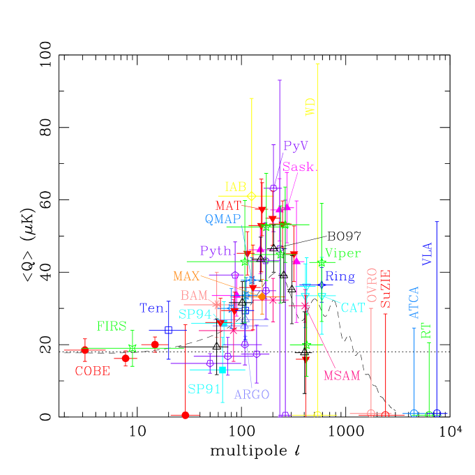
Figure 3: Most of the CMB anisotropy experiments published to date. See Smoot & Scott (1997) and Halpern & Scott (1999) for full references, supplemented with more recent results from: OVRO Ring (Leitch et al. 1999); QMAP (de Oliveira-Costa et al. 1998); MAT (a.k.a. TOCO, Torbet et al. 1999 and Miller et al. 1999); CAT (Baker et al. 1999); Python V (Coble et al. 1999); Viper (Peterson et al. 1999); and BOOMERanG NA (a.k.a. BOOM97, Mauskopf et al. 1999). The error bars (these are $1\sigma$ except for the upper limits which are 95%) have generally been symmetrised for clarity, and calibration uncertainties are included in most cases. The horizontal bars represent the widths of the experimental window functions. The dotted line is the flat power spectrum which best fits the COBE data alone. The dashed curve is the prediction from the vanilla-flavoured standard Cold Dark Matter model.

There have been around 20 separate experiments which have detected temperature fluctuations which are most likely to be primordial. These are summarized in Fig. 3. Here the $x$-axis is the spherical harmonic multipole, $\ell$. The temperature fluctuation field on the sky, excluding the monopole and dipole, can be decomposed into an orthogonal set of modes:

$${\Delta T\over T}\left(\theta,\phi\right)=\sum_{\ell=2}^{\infty}\sum_{m=-\ell}^{+\ell}a_{\ell m}Y_{\ell m}(\theta,\phi).$$ (3)

Since there is no preferred direction on the sky (e.g. Bunn & Scott 1999) the individual $m$s are irrelevant, and so the important information is contained in the power spectrum

$$C_{\ell}\equiv\left\langle\left|a_{\ell m}\right|^{2}\right\rangle.$$ (4)

Indeed if the perturbations are Gaussian, then this contains all the information. The conventional amplitude of the quadrupole is given as

$${Q^{2}\over T_{0}^{2}}\equiv{\sum_{m}\left|a_{\ell m}\right|^{2}\over 4\pi}={5C_{2}\over 4\pi}.$$ (5)

A ‘flat’ spectrum means one in which $\ell(\ell+1)C_{\ell}={\rm constant}$, and we can therefore define that constant in terms of the expectation value for the equivalent quadrupole $\left\langle Q_{\rm flat}\right\rangle$ – which is what is plotted as the $y$-axis in Fig. 3.

Each experiment quotes one (or in the best cases several) measures of power over a range of multipoles, and these can be quoted as ‘band powers’ or equivalent amplitudes of a flat power spectrum through some ‘window function’. The horizontal bars on the points are an indication of the widths of these window functions (see White & Srednicki 1996 and Knox 1999 for more details).

More complete references for the experiments can be found in, e.g. Smoot & Scott (1997), Halpern & Scott (1999), Scott (1999). And for more details on each experiment start with http://www.astro.ubc.ca/people/scott/cmb.html, or other similar web-pages.

5 ‘Amongst our Weaponry are such Elements as …’

The list of the things which we have already learned from the CMB is probably larger than expected. Several facts can immediately be gleaned from Fig. 3:

• The plot has become very crowded!

• The overall detection of anisotropy is at the ${\simeq}\,40\sigma$ level

• A flat power spectrum (horizontal dotted line) is a bad fit, at about the $20\sigma$ level

• There is clear evidence for a peak at $\ell\sim 200$

One thing to add is that despite the appearance of scatter in the plot, smooth curves exist which provide a perfectly good fit to all the results (with only one or two exceptions). In order to see the wood for the trees, I have provided a binned version of the data in Fig. 4.

We can learn about the large-scale properties of the Universe from a variety of different techniques: cosmic flows; distant supernovae; galaxy clustering; ages of globular clusters; measurements of $H_{0}$; direct estimates of $\Omega_{0}$; cluster abundance; cluster baryon fraction; Big Bang nucleosynthesis; Lyman forest fluctuations; and other things I’ve forgotten. We are now at the point where the CMB anisotropies are providing constraints at least as good as from these other approaches. CMB anisotropies are an ideal tool for attacking cosmological parameters, since they probe linear theory on large scales. There is a great deal more information to obtain before the CMB bottoms-out (due to the cosmic variance limit), and no reason to be particularly concerned that any unavoidable systematic effect will be a show-stopper. Certainly there is a great deal to learn from other approaches (e.g. Cosmic Flows) which provide complementary information, but it seems clear that soon there will be extraordinarily large amounts of cosmological data collected from the CMB sky.

Figure 4: The result of binning the available data (from Fig. 3 for example). More precisely, what was done was to split the multipoles into 16 bins between $\ell\,{=}\,2$ and $\ell\,{=}\,1000$, and to weight each experiment by the fraction of the window in each bin. The precise height of the peak depends to some extent on the choice of bins, on details of the window functions used, and on the weights given to individual experiments. The points here are not un-correlated, but provide a reasonable visual impression of the current data – more sophisticated treatments (e.g. Bond, Jaffe & Knox 1998) give similar results. The solid line is a $\Lambda$-dominated CDM model, with parameters which are consistent with most current cosmological constraints.

The first thing we learn from Figs. 3 and 4 is that our basic paradigm – to describe the large scale properties of the Universe, and the formation of structure within it – are in good shape. The prediction from the ‘straw man’ model, standard Cold Dark Matter (sCDM) is shown by the dashed line in Fig. 3. This model (which contains parameters which are all fixed at very round numbers) is hardly the best fit, but it does have the right general character. And it is easy to find models which fit the data much better, by tuning some of those parameters.

More detailed inferences from Fig. 4 can be listed as follows (for more details refer to the review article by Lawrence et al. 1999):

• Gravitational instability in a dark matter dominated universe grew today’s structure

• The Universe remained neutral until $z\,{\la}\,50$

• The CMB power spectrum peaks at $150\,{\la}\,\ell\,{\la}\,350$

• There are some (weak) constraints on particle physics at $z\,{\sim}\,1000$

• The large-scale structure of spacetime appears to be simple

I will not discuss most of these in detail, but let me return to the issue of the main CMB acoustic peak. Since the standard CDM model has its main peak at $\ell\,{\simeq}\,220$, and it is pushed to smaller scales in open models, then the data prefer $\Omega_{\rm tot}$ close to unity, and certainly bigger than the ${\sim}\,0.3$ implied by various dynamical studies. Rigorous analyses of the anisotropy data (e.g. Dodelson & Knox 1999, Melchiorri et al. 1999) arrive at similar conclusions. The CMB thus provides the strongest evidence that the Universe is flat (or at least, nowhere near as open as the amount of dynamically detected dark matter would suggest).

The height of the peak is somewhat greater than predicted for sCDM, but entirely consistent with several variants. Currently popular models with a cosmological constant tend to provide perfectly good fits to the CMB. The curve plotted in Fig. 4, shows one such flat model with $\Omega_{\Lambda}=0.6$ and a Hubble constant of $70\,{\rm km}\,{\rm s}^{-1}{\rm Mpc}^{-1}$.

Since the height of the first peak depends on a combination of parameters, then exactly what quantities are constrained depends on the parameter space being searched, as well as on the choice of additional constraints. Currently it is possible to constrain the matter density $\Omega_{\rm M}$ to ${\sim}\,\pm 0.1$ from the peak height, but that depends sensitively on the assumptions used. All this is expected to change as better data come in.

All of this parameter estimation depends on having the correct family of models to test. In fact it is clear that that models with adiabatic-type perturbations (i.e. where you perturb the matter and radiation at the same time in order to keep the entropy fixed) have the right kind of character to fit the data. On the other hand isocurvature-type models (where the matter and radiation get equal and opposite perturbations, so that the local curvature is unperturbed) tend to look poor – generically they have a ‘shoulder’ rather than a first peak, and then the highest peak is at much smaller scale (see e.g. Hu, Spergel & White 1997). While there are some loop-holes, it seems difficult to get isocurvature models to fit the current data. The basic thing to take away from Fig. 4 then is that adiabatic models (with roughly scale-invariant initial conditions) are in good shape, and that within this class of models the CMB data are beginning to put constraints on parameters.

6 ‘Is this the Right Room for an Argument?’

The most contentious conclusion from the current CMB data concerns the implications from the mechanism that generated the perturbations. Most people working in the field which is sometimes referred to as ‘CMB phenomenology’ are currently struggling with the same question, in one form or another: does the CMB data prove inflation? It seems clear that we are now in a position to say something beyond the Big Bang paradigm. The CMB led us to accept that the Universe used to be hotter and denser, and more recently to the conclusion that structure built up through gravitational instability. Now it appears that we are learning something further, something about the origin of the perturbations themselves. But just exactly what that next step is, and how to phrase it, is altogether less clear. For lack of anything better, let me present my own current belief, which I challenge anyone to disagree with:

• Something like Inflation is something like proven

The only causal way we know of to have adiabatic fluctuations on apparently acausal scales is to have the scale factor accelerate at some time in the early history of the Universe (e.g. Liddle 1995). And we can argue about whether something that achieves the same end result is just isomorphic to inflation, even if interpretted differently. Here ‘inflation’ does not necessarily carry with it the extra baggage of an inflaton potential etc. – although hopefully the connection with particle physics would follow later.

It used to be that discussions of inflation focussed on the number of e-foldings required to solve horizon, flatness, entropy and monopole problems. However, at the present time the paramount concern is making the density perturbations – and inflation gives you a mechanism to do that, for free. It appears that we are learning that the Universe has inflation-like ‘initial conditions’. Time will tell whether that means that the Universe was once dominated by some vacuum energy density, and whether we can learn details about particle physics at ultra-high energies.

7 ‘This is an Ex-Parrot’

Let me continue the contentious theme by saying a little something about the main competition for inflation – any one of various field ordering mechanisms or topological defect models. Generically these give larger CMB anisotropies, from the so-called integrated Sachs-Wolfe effect, for the same density perturbation amplitudes. This is basically because of their similarity to isocurvature models; adiabatic (i.e. inflationary) models, on the other hand, give the correct value to a factor of 2, without really trying. The power spectra of galaxy perturbations, or even the underlying dark matter fluctuations, are notoriously complicated to calculate in defect models – nevertheless there seems little hope that the observed power spectrum can be easily reproduced in these sorts of models. Moreover, there now seems to be some consensus in the view that generic defect models produce either one (broad) peak in a place which gives a poor fit to current data, or perhaps even no peak at all (Pen, Seljak & Turok 1997, Albrecht et al. 1997, Allen et al. 1997).

The status of defects vs. the Universe can be summarized in the following three points. Defect models tend to give: the wrong matter power spectrum; the wrong CMB power spectrum; and the wrong normalization of matter relative to CMB. But apart from that, these models seem to work fine!

Of course there is some motivation for working on such models simply because they cool – and indeed they may yet be important in other purposes in the early Universe – but at this point they seem to hold little promise as a method of forming structure.

8 ‘This Theory which Belongs to me is as Follows’

If we are close to proving something like inflation, then that may only be because the only serious competitor, defects, seems in such bad shape. It may be that we are just lacking in imaginative enough ideas, just waiting for a better theory to come along. So certainly it is worth investigating other possibilities, at least until such time as inflation has been more directly tested. While the current suite of defect models do not look very promising, there is always the possibility of a more attractive, related model lying around corner.

New ideas from particle physics also have the potential for providing different mechanisms for structure formation. Exactly what will come out of string theory, large extra dimensions and broken Lorentz invariance remains to be seen. It will be interesting to see how generic the basic inflationary predictions are, and whether new twists on high energy physics carry with them new testable predictions.

9 ‘That’s the Machine that Goes “Ping”’

That the field of CMB anisotropies is progressing rapidly is largely due to the experimental efforts. These are extremely difficult measurements to make, and to do so has required impressive developments in detector technology, as well as experimental strategies and data analysis methods. More information about current and future CMB experiments can be found in recent reviews (e.g. Lawrence 1998, Halpern & Scott 1999); here I give only a very brief summary.

The next generation of CMB balloon experiments are expected to return data of much higher quality (and quantity). The newest results from the North American test flight of BOOMERanG (‘BOOM97’, Mauskopf et al. 1999) are certainly impressive, and others (such as MSAM and MAXIMA) are eagerly awaited. BOOMERanG ‘98 was the first long-duration balloon flight, and by all accounts was staggeringly successful – BOOM98 seems likely to provide an enormous leap forward in anisotropy measurements. Three immediate questions are expected to be addressed by this new data-set: do the currently favoured $\Lambda$-dominated cosmologies continue to be a good fit; what is the precise location of the first peak; and is there any evidence for other peaks. This last point is perhaps the most important. Detection of oscillations in the power spectrum, with tight constraints on the peak spacings, will be a very firm test of the inflationary paradigm (Hu & White 1996).

The adiabatic, apparently acausal perturbations, generated during inflation, give a series of peaks in the ratio $1\,{:}\,2\,{:}\,3\,{:}\,\cdots$ in $\ell$-space. On the other hand, causal, isocurvature perturbations naturally give rise to peaks in the ratio $1\,{:}\,3\,{:}\,5\,{:}\,\cdots$. So detection of a second peak at roughly half the angular scale of the first, will be a very large step towards ‘proving inflation’. Failure to observe this will, of course, be even more exciting, since it will demand an entirely new paradigm.

In the short term there are also at least three new interferometer projects (e.g. White et al. 1999): DASI at the South Pole; CBI in Chile; and the VSA in Tenerife. All of these are nearing completion and should produce data within the next year or two.

Another direction being pursued from the ground is CMB polarization – see Staggs, Gundersen & Church 1999 for experimental details and Hu & White 1997 for a theory primer. The CMB sky is naturally polarized at the few percent level (the result of the quadrupole term in Compton scattering together with a slightly anisotropic radiation field at $z\,{\sim}\,1000$). Measuring the ${\sim}\,\mu$K signals will be very challenging, but can provide information beyond that contained in the temperature anisotropies alone. Since polarization is such a strong prediction, it better be there, otherwise our whole picture has to change! Furthermore, we can more definitively separate any gravity wave contribution in the CMB (if it is measurable, Zibin, Scott & White 1999), thus limiting the energy scale of inflation. Large-angle polarization can also constrain the reionization epoch, and details of the polarization power spectrum are a direct probe of physics around the time of last scattering. This is all in addition to the fact that polarization simply gives extra information to better constrain parameters (and to break degeneracies between some combinations of parameters).

Two satellite missions are currently planned to study the CMB from space, where the whole sky can be imaged, far from the complicating effects of the atmosphere. The NASA Microwave Anisotropy Probe (MAP ) is due for launch in November 2000. It will travel to the Earth-Sun outer Lagrange point, L2, where it will map the sky at 5 frequencies between 22 and $90\,$GHz, reaching to $\ell\,{\sim}\,800$ in the power spectrum. The careful control of systematics possible with an extended space mission means that MAP should represent a very large improvement over the data available from the Earth-based experiments.

Figure 5: An estimate for how well the power spectrum might be measured by Planck. This is a realization of a CDM power spectrum, assuming the Planck instrumental sensitivity over two thirds of the sky. Planck should supply us with essentially cosmic-variance limited information on all the angular scales relevant to primary anisotropies, over the full range of relevant frequencies.

The ESA mission Planck can be thought of as the third generation CMB satellite, mapping at 9 separate frequencies between 30 and $850\,$GHz, with both radiometer and bolometer technologies, and measuring the $C_{\ell}$s to beyond $\ell$ of 2000. Thus Planck is expected to measure essentially all of the primordial CMB power spectrum (see Fig. 5), and cover all the frequencies required to measure and remove the foreground signals. The Planck data set should enable cosmological parameters to be constrained with exquisite precision – or, to put it another way, the power spectrum should be measured at a level of several million $\sigma$. In addition Planck will measure the polarization (and cross-correlation with temperature) power spectra, providing even more information.

Beyond MAP and Planck we might want to think about polarization, about small angular scales and about a ‘CMB Deep Field’ (see Halpern & Scott 1999 for discussion). Diffuse ‘foreground’ emission (from the Galaxy as well as more distant sources) is also likely to be studied more actively, as the ability to measure and identify these signals develops. Non-Gaussian signals from higher-order effects at small-scales would be expected to show up in fine-scale maps.

What will be the outcome of all this data? Certainly cosmological parameters will be well constrained. And definitely some messy astrophysical details will be uncovered (in the foregrounds, as well as through some weak processing effects occurring between $z\,{=}\,0$ and 1000). And whatever the basic paradigm, there will surely be some clues to fundamental physics lurking in there, since the CMB anisotropies provide the cleanest information about the initial conditions and the largest scale properties of the Universe.

10 ‘Exciting? No it’s not. It’s Dull, Dull, Dull’

If one looks at what is currently known about cosmological parameters, then depending on one’s mood there are 2 possible conclusions: (1) it is extremely difficult to measure these things properly, and so the jury is still out; or (2) we already have a fairly clear picture of the Universe. I personally lean more towards the former (at least on Mondays, Wednesdays and Fridays). If we take the consensus, inflationary, $\Lambda$-dominated models seriously, then we would conclude that all of the parameters ($\Omega_{\rm DM}$, $\Omega_{\rm B}$, $H_{0}$, $n$, $t_{0}$, negligible tensors, reionization, non-adiabatic modes, no-Gaussianity, etc.) are known with errors of perhaps 10–20%. It would be not only extremely surprising if we were to find ourselves in that position, but also extremely boring!

Let us fervently hope that the Universe is smarter than the smartest theorist of the day, and is keeping something up its sleeve. Otherwise we will be reduced to measuring a bunch of model parameters to ever greater precision. Still, it is very hard to believe that ‘the end of cosmology’ is really in sight. Rather than expecting MAP, Planck and the rest to be giving us 10 parameters to 1% accuracy, let us look forward to the surprises that are in store for us.

11 ‘And Finally, Monsieur, a Wafer-Thin Mint’

We are beginning to learn the answers to some fundamental questions, using information contained in CMB anisotropy data. The CMB has already made it clear that gravitational instability was sufficient to grow all the structure in the Universe. Most recently it has been providing strong evidence that the Universe is nearly flat. Soon we can expect (through the existence or lack of oscillations in the power spectrum) a direct test of the inflationary scenario. With future experiments, such as long-duration balloons, interferometers, and the MAP and Planck satellites, we should expect to learn vastly more in the coming years about particle physics, cosmology and astrophysics.

- [1] lbrecht, A., Battye, R. A., & Robinson, J., 1997, Phys. Rev. Lett.79, 4736 [astro-ph/9707129]
- [2] llen, B., et al. 1997, Phys. Rev. Lett., 79, 2624 [astro-ph/9704160]
- [3] aker, J. C., et al., 1999, MNRAS, 308, 1173 [astro-ph/9904415]
- [4] arger, A. J., Cowie, L. L., & Sanders, D. B., 1999, ApJ, 518, L5 [astro-ph/9904126]
- [5] lain, A. W., Kneib, J.-P., Ivison, R. J., & Smail, I., 1999, ApJ, 512, L87 [astro-ph/9812412]
- [6] ond, J. R., Crittenden, R., Davis, R. L., Efstathiou, G., & Steinhardt, P. J., 1994 Phys. Rev. Lett.72, 13
- [7] ond, J. R., Jaffe, A. H., & Knox, L. E., 1998, ApJ, in press, [astro-ph/9808264]
- [8] unn, E. F., & Scott, D., 1999, MNRAS, in press [astro-ph/9906044]
- [9] hapman, S. C., Scott, D., Borys, C., & Fahlman, G. G., 1999, in preparation
- [10] oble, K., et al., 1999, ApJ, 519, L5 [astro-ph/9902195]
- [11] ourteau, S., & van den Bergh, S., 1999, AJ, 118, 337 [astro-ph/9903298]
- [12] e Oliveira-Costa, A. et al., 1998, ApJ, 509, L77 [astro-ph/9808045]
- [13] odelson, S., & Knox, L., 1999, Phys. Rev. Lett., submitted [astro-ph/9909454]
- [14] ole, H., et al., 1999, The Universe as seen by ISO, ed. P. Cox, M.F. Kessler, UNESCO, Paris, ESA SP-427, in press [astro-ph/9902122]
- [15] wek, E., & Arendt, R. G., 1998, ApJ, 508, L9 [astro-ph/9901045]
- [16] ales, S., et al., 1999, ApJ, 515, 518 [astro-ph/9808040]
- [17] ixsen, D. J. et al., 1996, ApJ, 473, 576 [astro-ph/9605054]
- [18] ixsen, D. J., Dwek, E., Mather, J. C., Bennett, C. L., & Shafer, R. A., 1998, ApJ, 508, 123 [astro-ph/9803021]
- [19] endreau, K. C., et al., 1995, PASJ, 47, L5
- [20] uiderdoni, B., Hivon, E., Bouchet, F.R., & Maffei, B., 1998, MNRAS, 295, 877 [astro-ph/9710340]
- [21] aiman, Z., & Knox, L., 1999, ApJ, in press [astro-ph/9906399]
- [22] alpern, M., & Scott, D., 1999, Microwave Foregrounds, ed. A. de Oliveira-Costa & M. Tegmark, ASP, San Francisco [astro-ph/9904188]
- [23] auser, M. G., et al., 1998, ApJ, 508, 25 [astro-ph/9806167]
- [24] u, W., Scott, D., Sugiyama, N., & White, M., 1995, Phys. Rev. D, 52, 5498 [astro-ph/9505043]
- [25] u, W., Spergel, D. N., & White, M., 1997, Phys. Rev. D, 55, 3288 [astro-ph/9605193]
- [26] u, W, & White, M., 1996, Phys. Rev. Lett., 77, 1687 [astro-ph/9602020]
- [27] u, W, & White, M., 1997, NewA, 2, 323 [astro-ph/9706147]
- [28] ughes, D., et al., 1998, Nature, 394, 241 [astro-ph/9806297]
- [29] ungman, G., Kamionkowski, M., Kosowsky, A., & Spergel, D. N., 1995 [astro-ph/9507080]
- [30] appadath, S. C., et al., 1999, HEAD, 31, 3503
- [31] awara, K., et al., 1998, A&A, in press
- [32] nox, L., 1999, Phys. Rev. D, 60, 103516 [astro-ph/9902046]
- [33] agache, G., Abergel, A., Boulanger, F., Désert, F. X., & Puget, J.-L., A&A, 344, 322 [astro-ph/9901059]
- [34] agache, G., & Puget, J.-L., 1999, A&A, in press [astro-ph/9910255]
- [35] awrence, C. L., 1998, in ‘Evolution of Large Scale Structure’, ed. A.J. Banday et al., in press,
- [36] awrence, C. L., Scott, D., & White, M., 1999, PASP, in press, [astro-ph/9810446]
- [37] einert, C. H., et al., 1998, A&AS, 127, 1
- [38] eitch, E. M., et al., 1999, ApJ, in press [astro-ph/9807312]
- [39] iddle, A. R., 1995, Phys. Rev. D, 51, 5347 [astro-ph/9410083]
- [40] ineweaver, C. H., et al., 1996, ApJ, 470, 38 [astro-ph/9601151]
- [41] onsdale, C. J., Hacking, P. B., Conrow, T. P., & Rowan-Robinson, M., 1990, ApJ, 358, 60
- [42] adau, P., & Pozzetti, L., 1999, MNRAS, in press [astro-ph/9907315]
- [43] ather, J. C., Fixsen, D., Shafer, R. A., Mosier, C., & Wilkinson, D. T., 1999, ApJ, 512, 511 [astro-ph/9810373]
- [44] auskopf, P. D., et al., 1999, ApJ, in press [astro-ph/9911444]
- [45] elchiorri, A., et al., 1999, ApJ, in press [astro-ph/9911445]
- [46] iller, A. D. et al., 1999, ApJ, 524, L1 [astro-ph/9906421]
- [47] iyaji, T., et al., 1998, A&A, 334, L13 [astro-ph/9803320]
- [48] liver, S., et al., 1997, MNRAS, 847, 1 [astro-ph/9707029]
- [49] en, U.-L., Seljak, U., & Turok, N., 1997, Phys. Rev. Lett., 79, 1611 [astro-ph/9704165]
- [50] eterson, J. B., et al., 1999, ApJ, in press [astro-ph/9910503]
- [51] ozzetti, L., Madau, P., Zamorani, G., Ferguson, H. C., & Bruzual, G. A., 1998, MNRAS, 298, 1133 [astro-ph/9907315]
- [52] essell, M. T., & Turner, M. S., 1990, Comments Astrophys., 14, 323
- [53] ush, B., Malkan, M. A., & Spinoglio, L., 1993, ApJS, 89, 1
- [54] charfe, C. A., et al., 1999, ApJ, submitted [astro-ph/9908187]
- [55] cott, D., et al., 1999, A&A, submitted [astro-ph/9910428]
- [56] cott, D., Silk, J., & White, M., 1995, Science, 268, 829 [astro-ph/9505015]
- [57] cott, D., & White, M., 1999, A&A, 346, 1
- [58] eager, S., Sasselov, D., & Scott, D., 1999, ApJ, 523, L1 [astro-ph/9909275]; ApJ, in press [longer paper]
- [59] eljak, U., & Zaldarriaga, M., 1996, 469, 437 [astro-ph/9603033]
- [60] moot, G. F., et al., 1992, ApJ, 396, L1
- [61] moot, G. F., 1997, Proc. of the Strasbourg NATO School, in press [astro-ph/9705101]
- [62] moot, G. F., & Scott, D., 1998, in Caso C., et al., Eur. Phys. J., C3, 1, the Review of Particle Physics, p. [astro-ph/9711069]
- [63] reekumar, P., et al., 1998, ApJ, 494, 523 [astro-ph/9709257]
- [64] taggs, S. T., Gundersen, J. O., & Church, S. E., 1999, Microwave Foregrounds, ed. A. de Oliveira-Costa and M. Tegmark, ASP, San Francisco [astro-ph/9904062]
- [65] orbet, E., et al., 1999, ApJ, 521, L79 [astro-ph/9905100]
- [66] reyer, M., et al., 1998, ApJ, 509, 531 [astro-ph/9801293]
- [67] eidenspointner, G., et al., 1999, Astronomische Gesellschaft Meeting, 15, 102
- [68] hite, M., Carlstrom, J. E., Dragovan, M., & Holzapfel, S. W. L., 1999, ApJ, in press [astro-ph/9712195]
- [69] hite, M., Scott, D., & Silk, J., 1994, ARA&A, 32, 319
- [70] hite, M., & Srednicki, M., 1995, ApJ, 443, 6 [astro-ph/9402037]
- [71] ibin, J. P., Scott, D., & White, M., 1999 Phys. Rev. D, in press [astro-ph/9901028]