LINE EMISSION FROM STELLAR WINDS
IN ACTIVE GALACTIC NUCLEI

Line Emission in Active Galactic Nuclei II: Fitting Orbital Cloud Models with Variability Data

Abstract

This dissertation presents synthetic spectra and response functions of the red giant stellar line emission model of active galactic nuclei (e.g., Kazanas 1989). Our results agree with the fundamental line emission characteristics of active galactic nuclei within the model uncertainties if the following new assumptions are made: 1) the mean stellar mass loss rates decrease with distance from the black hole, and 2) the mean ionization parameters are lower than those postulated in Kazanas (1989). For models with enhanced mass loss, the zero-intensity-full-widths of the line profiles are proportional to the black hole mass to the power of 1/3. This scaling relation suggests that the black hole masses of NLS1s (narrow-line Seyfert 1s) are relatively low. Models with enhanced mass loss also predict minimum line/continuum delays that are proportional to the zero-intensity-full-widths of the profiles. Because of their high column densities, these models yield triangle-shaped response functions, which are not generally observed. On the other hand, models without enhanced mass loss yield line-continuum delays that are proportional to the square root of the continuum luminosity. This prediction appears to agree with results from reverberation mapping campaigns.

If the intercloud (interstellar) medium densities are high enough, the winds are “comet shaped,” with the shock fronts having higher densities than the cloud “tails.” In this case, the densities in the ionized (inverse Strömgren regions) of the outbound clouds are lower than those of the inbound clouds. For models in which an accretion disk occults the broad line region, the broadest line emission and absorption profile components of lines similar to C IV, N V, and O VI are redshifted. Conversely, the narrowest emission and absorption profile components are blueshifted. The shifts of the Lyman alpha profile components are much smaller. One particularly interesting prediction of the nonspherical wind models is that their C IV red wings respond faster than their blue wings, as has been observed (e.g., Done & Krolik 1996). These same models, however, yield opposite results for the C III] line, such that the C III] blue wings respond first. For this reason, measurements of the velocity dependence of the C III] profile response could be used to test the viability of nonspherical stellar wind line emission models.

secnumdepth5 tocdepth5

Laboratory of High Energy Astrophysics
NASA Goddard Space Flight Center Dr. Demosthenes Kazanas Professor Jordan A. Goodman, Chair
Professor Abolhassan Jawahery
Dr. Timothy Kallman
Professor Dennis Papadopoulos
Professor Andrew S. Wilson preface In memory of David Waylonis, who taught me the importance of uncovering the truth.

Chapter 1 Introduction

1.0“What you have to do, if you get caught in this gumption trap of value rigidity, is slow down—you’re going to have to slow down anyway whether you want to or not—but slow down deliberately and go over ground that you’ve been over before to see if the things you thought were important were really important and to . . . well . . . just stare at the machine. There’s nothing wrong with that. Just live with it for a while. Watch it the way you watch a line when fishing and before long, as sure as you live, you’ll get a little nibble, a little fact asking in a timid, humble way if you’re interested in it. That’s the way the world keeps on happening. Be interested in it.

At first try to understand this new fact not so much in terms of your big problem as for its own sake. That problem may not be as big as you think it is. And that fact may not be as small as you think it is. It may not be the fact you want but at least you should be very sure of that before you send the fact away. Often before you send it away you will discover it has friends who are right next to it and are watching to see what your response is. Among the friends may be the exact fact you are looking for.

After a while you may find that the nibbles you get are more interesting than your original purpose of fixing the machine. When that happens you’ve reached a kind of point of arrival. Then you’re no longer strictly a motorcycle mechanic, you’re also a motorcycle scientist, and you’ve completely conquered the gumption trap of value rigidity.

…

I can just see somebody asking with great frustration, ‘Yes, but which facts do you fish for? There’s got to be more to it than that.’

But the answer is that if you know which facts you’re fishing for you’re no longer fishing. You’ve caught them.”

—Robert M. Pirsig

1.1 Background

1.5Galaxies are composed of stars. Most of these stars emit Plank continua with myriad absorption lines. It is, therefore, understandable that the spectra of galaxies also have absorption lines. But in 1908, before the distances to “spiral nebulae” had even been determined, Edward A. Fath discovered line emission from the center of the nearby spiral nebula M77, more commonly known as NGC 1068 (Fath 1909). NGC 1068 is now categorized as an “active” galaxy. To this day, there is still no consensus on what produces the lines emitted by NGC 1068 and similar active galaxies.

The centers of $\approx 46$% of all galaxies are active in that they emit at least some form of line emission or nonthermal continuum radiation (Ho 1996). A picture of the active galaxy NGC 5548 taken by the Hubble Space Telescope (HST) WFPC2 camera is shown in

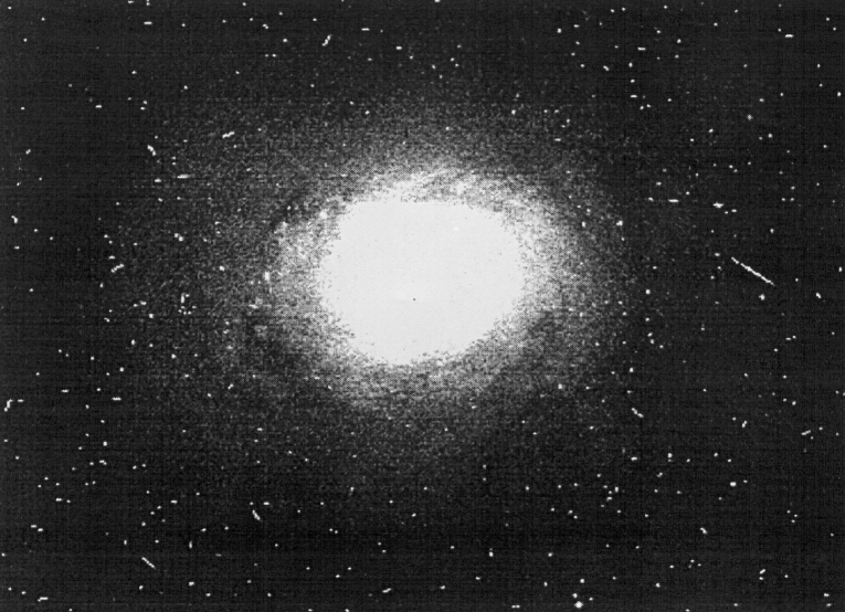
Figure 1.1: WFPC2 image of active spiral galaxy NGC 5548. This galaxy has a redshift of $z=0.0174$, placing it $7\times 10^{7}$ pc ($2.3\times 10^{8}$ light-years or $2.2\times 10^{26}$ cm) away from us if a Hubble constant of 75 km s^-1 Mpc^-1 (where Mpc is an abbreviation for 10⁶ parsecs) is assumed and all non-cosmological motions are neglected.

Figure 1.1. The unresolved central continuum source in NGC 5548 is brighter in the ultraviolet (UV) than the entire remainder of the galaxy. The UV spectrum of the entire galaxy is, therefore, quite similar to the central source. This spectrum is shown in

Figure 1.2: Time-averaged UV spectrum of AGN NGC 5548 obtained from the HST FOS. Data courtesy of K. Korista.

Figure 1.2. The majority of AGNs have only narrow (equivalent Doppler shifts of $c\Delta\lambda/\lambda_{0}\mathrel{\hbox{\hbox to0.0pt{\hbox{\lower 5.0pt\hbox{$\sim$}}\hss}\hbox{$<$}}}$ 1000 km s^-1) lines superimposed upon a nonthermal continuum. NGC 5548 is one of the $\sim$20% of AGNs (Ho 1996) that is also a Seyfert 1, with larger line widths of $\Delta\lambda/\lambda_{0}\sim 0.02$. Seyfert 1s and their brighter counterparts called quasars (also known as “QSOs”) are the primary topic of this dissertation. They are AGNs with line emission profiles that are very broad (equivalent Doppler shifts of $\sim$ 5000 km s^-1), but their profiles may also contain the narrower profile components that are more commonly observed. In Seyfert 1s, the broad profile components are readily apparent in the UV spectral region due to their large equivalent widths of $\sim 10$ Å ($1.0$ Å$\equiv 10^{-10}\textrm{ m}$). Several other AGN categories have been invented. For instance, AGNs that are extremely bright in the radio band are known as radio-loud AGNs. This category constitutes 10% of all Seyfert 1s. One such radio-loud AGN is M87, shown in Figures 1.3 and 1.4.

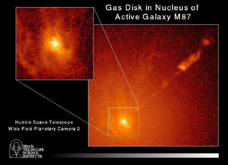
Figure 1.3: WFPC2 image of supermassive active elliptical galaxy M87, center of the Virgo, the nearest cluster of galaxies. Upper right: the near side of a jet protruding perpendicularly out of a dusty disk toward us from the continuum source. Photo courtesy of STScI.

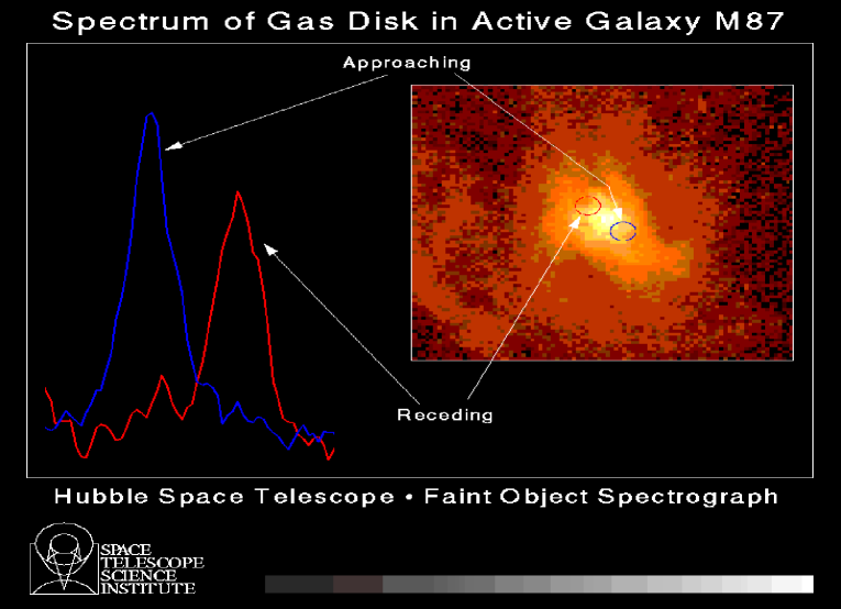
Figure 1.4: Right: blowup of central disk in M87. Left: superimposed spectra of two regions of the disk illustrating Doppler shifts of the [O III] $\lambda\lambda$4959, 5007 doublet. Photo courtesy of STScI.

Although 90 years have elapsed since Fath’s original publication, the mystery of what produces the narrow and broad line emission remains unsolved. Recent space-based observations have literally shed new light on the problem by making UV spectra available for the first time. This has fueled research; 14% of all 1995 Astrophysical Journal papers mention “AGN” in their abstract.

Before discussing the Seyfert 1 and QSO AGN models that have been proposed to date, let us first review what is generally suspected about AGNs. This review will provide perspective and reduce the chance that we box ourselves into a narrow corner of model parameter space. Because there is so little consensus in the field, let us begin at the beginning, with the suspected formation of AGNs and their host galaxies.

Before galaxies formed, there were density and velocity fluctuations left over from the big bang. As gravitational attraction pulled the higher density regions together, protogalaxies with even higher densities began to form. These protogalaxies had small velocity gradients induced by tidal torques from neighboring protogalaxies. Because gas is inherently dissipative (both collisional and inelastic), its orbits cannot cross. For this reason, the gas in the protogalaxies formed disks that had axes aligned with the initial average angular momentum vectors. If viscous forces can be neglected, the distance between protogalaxies is small compared to the initial velocity perturbation scale length, and star formation does not consume most of the gas prior to its collapse, then it can be shown that conservation of angular momentum yields a post-collapse disk surface density of

$$\Sigma(r)={G\over r}\left({\rho d_{{\rm g}}\over|\nabla\times{\bf{v}}|}\right)^{2}.$$ (1.1)

In this equation, $r$ is the galactic radius, $G$ is the gravitational constant, $\rho$ is the initial mean cosmological density near the protogalactic center of mass, $d_{{\rm g}}$is the initial distance between protogalaxies, and $\nabla\times{\bf{v}}$ is the curl of the initial velocity function of the gas near the protogalactic center of mass. Relations similar to equation (1.1) were first derived by Mestel (1963, 1965) and have since been verified by numerical calculations (e.g., Fall & Efstathiou 1980). Though it is currently a matter of debate as to what the dominant contributor of mass in galaxies is, the surface density of equation (1.1) yields a flat rotation curve and a divergent density at $r=0$. But an initial assumption made in deriving equation (1.1) was that viscous forces could be neglected. Since the importance of viscosity increases sharply with density, equation (1.1) must be violated near $r=0$. Such viscosity would force the formation of and the rapid accretion onto a compact object such as a supermassive black hole not unlike the one suspected of residing in M84 (see

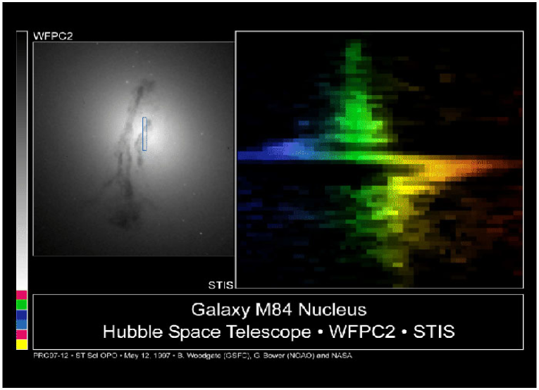
Figure 1.5: Left: photograph of nearby galaxy M84. Right, vertical axis: position within central boxed region in photograph on left. Right, horizontal axis: equivalent line-of-sight velocity of line peaks in position-dependent spectrum within boxed region. The “S” shape is suggestive of a supermassive black hole. Photo courtesy of STScI.

Figure 1.5). The gravitational potential energy that must be released for this accretion process to occur is sufficient to power the continuum energy released by the high-redshift quasars we see today.

1.2 A Critique of AGN Line Emission Models

Though the accretion disk theory of AGN continuum emission currently has little “competition,” there is no consensus on the AGN line emission models. The following is a an incomplete list of the models that have been proposed:

• Non-Doppler line broadening (e.g., Raine & Smith 1981, Kallman & Krolik 1986)

• Two-phase, pressure-equilibrium clouds in radial flows or chaotic motions (e.g.; Wolfe 1974; McCray 1979; Krolik, McKee, & Tarter 1981)

• Accretion disks with central tori or coronas (e.g., Collin-Souffrin 1987, Eracleous & Halpern 1994)

• Hydromagnetically driven outflows from accretion disks (e.g., Emmering, Blandford, & Shlosman 1992; Cassidy & Raine 1993)

• Outflowing disk winds (Murray et al. 1995)

• Stellar winds (e.g., Edwards 1980, Norman & Scoville 1988, Kazanas 1989, Alexander & Netzer 1994)

• Tidally disrupted stars (e.g., Roos 1992)

• Supernovae remnants (e.g., Aretxaga, Fernandes, & Terlevich 1997)

The next several subsections comment on the viabilities of some of these models.

1.2.1 Non-Doppler Broadening?

Before a species as questionable as “rapidly moving broad line region cloud” (hereafter, “BLR cloud”) is considered seriously in order to describe AGN line emission, one should first estimate the importance of the non-Doppler broadening mechanisms. Such estimates are also useful in estimating the minimal number of clouds that some AGN models require. As discussed in §§  2.1 & 1.3, this is because AGN emission profiles are observed to be extremely smooth.

There are several different potential sources of line broadening in AGNs. Let us discuss some of the most important. The existence of a broad, yet relatively weak component of the C III] $\lambda$1909 inter-combination line (where the number after “$\lambda$” represents the transition wavelength in units of Å) suggests electron densities for the BLR edge surfaces (as defined by the positions in the line-emitting region where the optical depths to the observer are $\sim$3/4) of the BLR emission gas (more specifically, a plasma) of $\sim 10^{11}$ cm^-3 (e.g. Ferland et al. 1992). For the lines AGNs are observed to emit, such densities are too low for Stark broadening (also referred to as pressure broadening) to yield profiles as broad as 5000 km s^-1. Another argument against Stark broadening as being the dominant source of the line broadening in AGNs is the overall similarity between the various lines. Stark broadening would generally predict a different profile width for each line. The opposite trend is observed (see, e.g., Laor et al. 1994).

One non-Doppler broadening mechanism which does predict similar profile shapes for different transitions is electron scattering (e.g., Raine & Smith 1981, Kallman & Krolik 1986). Electron scattering becomes important for electron column densities greater than $\sim\sigma_{{\rm T}}^{-1}=1.5\times 10^{24}$ cm^-2, where $\sigma_{{T}}$ is the Thomson cross section.

One important feature of AGNs is that their continua luminosities vary as a function of time. The lines are also observed to vary. Because the gas emitting the lines is expected to be heated by the continuum, this line variation is expected. The lines, however, take a finite time to respond to the changes in the continuum. Line/continuum delays are discussed in much more detail in § 2.2. Electron scattering models predict a minimum variability time for both the lines and the continua of $\tau\sim r_{{\rm BLR}}/c$, where $c$ is the speed of light and $r_{{\rm BLR}}$ is the frequency-dependent radius where the electron scattering optical depth to the observer is 3/4. The continuum-subtracted line emission does not appear to have the same minimum time scales as their underlying continua at the same frequency. In fact, the UV lines are observed to take approximately 2-6 times longer to vary than the UV continua (see Fig. 1.7). Thus, electron scattering is probably not the dominant source of line broadening in AGNs.

For these reasons, non-Doppler line broadening is unlikely to be the dominant broadening mechanism for most of the strong and broad AGN UV lines.

1.2.2 Clouds in Pressure Equilibrium With a Hot, Intercloud Medium?

Many papers published between 1985 and 1992 refer to the “standard model” of AGN line emission. This standard model is the pressure-equilibrium model developed by Wolfe (1974), McCray (1979), and Krolik, McKee, & Tarter (1981). The model assumes cool, high-density regions called clouds which have temperatures of $\sim$ 10⁴ K embedded in a much larger, hot, $\sim$ 10⁸ K, intercloud medium. Because line emission becomes a relatively inefficient coolant at high enough temperatures, the dependence of the equilibrium temperature upon ionization permits the two phases to exist in adjacent pressure equilibrium. The clouds and their confining medium are then assumed to be in either radial or chaotic motions at velocities of $v\sim c\Delta\lambda/\lambda_{0}$, where $\Delta\lambda$ is the approximate line width and $\lambda_{0}$ is the laboratory wavelength of the transition. An essential element of the pressure-equilibrium model is that it assumes a very low filling factor. That is, most of the BLR region is assumed to be of very low density. This is compatible with several empirical features of AGNs, including the fact that the continua (emitted by accretion disks around the black holes) are able to vary much faster than the lines (emitted by the clouds which are much farther away from the black hole). Another feature of the pressure-equilibrium cloud model is its compatibility with several of the observed line ratios. This agreement indicates that the plasma emitting the lines is photoionized primarily by the continuum source and is not in LTE (local thermal equilibrium).

One can distinguish between two quite different types of pressure-equilibrium cloud models. The original pressure-equilibrium cloud model assumed that the inter-cloud medium is co-moving with the clouds. Several authors have, however, also assumed clouds that move within the intercloud medium. Let us consider each of these types of models in turn.

For models in which the clouds are co-moving with the intercloud medium, the kinematic structure of the intercloud medium is important. As mentioned previously, gas is dissipative. As a result, unless special external forces such as magnetic fields act upon it, any local velocity gradients within an intercloud medium would quickly die out. If magnetic forces are important, however, the clouds are probably confined by the magnetic fields, not the intercloud medium pressure. This would violate the fundamental assumption of the gas pressure-equilibrium cloud model. Thus, the intercloud medium in the pressure-equilibrium model either should fall into the accretion disk or be in radial motion. Line emission from disks is discussed in §§ 1.2.3-1.2.4. Radial motion is ruled out in objects like NGC 4151 by red versus blue wing variability studies (see, e.g., Maoz et al. 1991). AGNs are noted for their conformity over extreme variations in parameter space, so it is unlikely that this object is an exception.

But this is just one of many problems with the co-moving pressure-equilibrium model. The accretion efficiency can be estimated from the observed AGN luminosities and the mass flux. The mass flux is a simple function of the required radial velocities of the gas in such models (which must be roughly the same as the observed line widths) and the estimated density of the line-emitting gas (see § 1.2.1). The mass flux rates for the co-moving inter-cloud models are over $10^{3}$ $M_{\odot}$ yr^-1 (Kallman et al. 1993), where “$M_{\odot}$” denotes the solar mass unit. This mass flux is simply too large for most concepts involving AGNs to make sense; it implies accretion efficiencies of $10^{-5}-10^{-7}$. This efficiency is not only much less than the typically assumed efficiency of an accretion disk $(\sim 0.3mc^{2})$, but is even less than the efficiency of fusion $(\sim 10^{-3}mc^{2})$. For these reasons, pressure-equilibrium models in which the clouds are co-moving with the intercloud medium are poor BLR candidates.

Let us now consider pressure-equilibrium models in which the clouds are not co-moving with the intercloud medium. It is now believed that the clouds in these models would be disrupted by instabilities at an especially high rate. Updated estimates of the temperatures of the intercloud medium temperatures are only $\sim 10^{7}$ K; the implied inter-cloud densities are high enough that the ram pressure at the leading edge of a cloud should cause rapid breakup of the clouds due to Rayleigh-Taylor instabilities, unless the medium is co-moving with the clouds (Mathews & Blumenthal 1977; Allen 1984; Mathews & Ferland 1987). Krinsky & Puetter (1992) showed that the outer edges of even the co-moving clouds are unstable to a thermal instability which grows on times scales of $\sim$10³ s, which corresponds to evaporation times scales of $\mathrel{\hbox{\hbox to0.0pt{\hbox{\lower 5.0pt\hbox{$\sim$}}\hss}\hbox{$>$}}}10$ years. Krinsky & Puetter (1992) also found that the clouds are dynamically unstable to trapped Ly$\alpha$ radiation with growth times of $10^{6}$ s. If the covering factor is $\sim$0.1, these numbers imply $10^{6}$ cloud births per year. It is questionable that the proposed cloud formation mechanisms (e.g., Eilek & Caroff 1979; Beltrametti 1981; Krolik 1988; Emmering, Blandford, & Shlosman 1992) would be able to compete with these high disruption rates, especially without the co-moving assumption. Even if cloud generation did not require conditions different from those in the BLR and radial models somehow worked, how exactly what the clouds are and why they would be created with the required velocities is unclear.

But perhaps the most severe problem with the non-co-moving pressure-equilibrium model is simply that the clouds would slow down in $\sim$1.0 days as they transfer their momenta to the intercloud medium (Taylor 1996). The energy released by this process if the intercloud medium pressure were actually as high as the cloud pressure would be quite high. This is shown quantitatively in

Figure 1.6: Solid line: approximate power received per stellar wind (or cloud) for model 2 by continuum heating. These results are dependent upon the characteristics and parameters of model 2, which is a sub-Eddington AGN model discussed in detail in Chapter 4. Dotted line: the approximate power $P_{\rm d}$ due to the effects of drag. This calculation assumes that $P_{\rm d}=A\rho_{\rm HIM}<v^{2}>^{3/2}$, where $A$ is the cloud cross sectional area, $\rho_{\rm HIM}$ is the mass density of the intercloud medium, $<v^{2}>$ is the squared velocity dispersion of the clouds. It also assumes that the inter-cloud temperature is $T_{\rm HIM}=10^{7}$ K, the mean molecular weight per HIM particle is 1.3, and the inter-cloud pressure is the same as the cloud pressure. For radii below $\sim$1 light-days and greater than $\sim$ 10⁶ light days, neither $P_{\rm d}$ nor $<v^{2}>$ are defined for model 2 because there are no line-emitting objects in this region.

Figure 1.6. For this reason, drag was at one point even proposed to power AGN line emission. An argument against this idea (and the non-co-moving pressure-equilibrium model as well) is that the lines of some AGNs would probably be unable to respond substantially to changes in the continuum. This predicament is, therefore, similar to that of electron scattering (§ 1.2.1) in that it is largely incompatible with the observed characteristics of line variability.

In summary, though the pressure-equilibrium cloud model is able to match most of the line ratios reasonably well, its other problems appear to make it untenable.

1.2.3 Modified Accretion Disks?

There are several different types of accretion disk AGN BLR models. Most assume that the accretion disks producing the continua also produce the UV and optical lines. Before discussing the BLR models of modified accretion disks, let us first review the standard Shakura & Sunyaev (1973) accretion disk theory and why accretion disks were not originally expected to be important sources of AGN line emission.

Because the kinetic energy of matter in Keplerian motion must be -1/2 of the gravitational potential energy, the heating per unit surface area due to viscosity in an accretion disk is required to scale as $r^{-3}$, where $r$ is the distance from the black hole. This function has a very steep slope. The slope is so steep, in fact, that most of the emission would be emitted near the innermost emission region, which is generally assumed to be $\sim 3r_{{\rm S}}$, where $r_{{\rm S}}$ is the Schwarzschild radius. The temperatures on the $z=0$ plane inside accretion disks are slightly more uncertain, but if we assume each annulus to emit similar to a blackbody, we obtain (see, e.g., Pringle 1981)

$$T\sim 3.5\times 10^{6}(r/r_{{\rm S}})^{-3/4}\,\textrm{K}$$ (1.2)

assuming accretion at 10% of the Eddington limit and a black hole mass of 10${}^{8}M_{\odot}$. Thus, the region of continuum emission from a normal AGN accretion disk depends upon the frequency, with the regions emitting optical continuum radiation being much farther out than the regions near the Schwarzschild radius responsible for the “big, blue” $\nu F_{\nu}$ bump. Nevertheless, equation (1.2) predicts that even the optical continuum of typical AGNs should be emitted from a region less than several light days from the continuum source. Partial support of equation (1.2) is provided by time-sampled AGN data such as that shown in

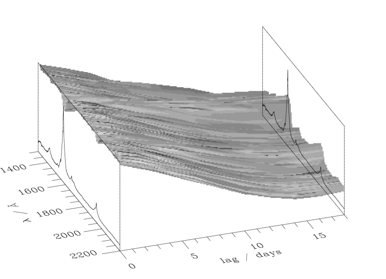
Figure 1.7: The $\tau\geq 0$ frequency-dependent cross correlation function between the 1135-1180 Å de-redshifted continuum and the UV spectral region of NGC 5548, an $M_{{\rm h}}\mathrel{\hbox{\hbox to0.0pt{\hbox{\lower 5.0pt\hbox{$\sim$}}\hss}\hbox{$<$}}}10^{8}$ AGN. This plot was made using the AGN watch (Alloin et al. 1994) HST variability campaign data described in Korista et al. (1995).

Figure 1.7. These data show that the lines respond on a distinctly different, and in particular longer, time scale than the underlying continuum. They also show that the $\lambda$2200:1160 Å continuum emission variability time lag, which according to equation (1.2) should be about twice as long as the underlying $\lambda$1300 Å variability time scale, is still too short to be detected with this data, which has a sampling rate of 3 days. Models which would emit substantial UV continua from equivalent distances farther than this are clearly ruled out.

For various reasons, the line-emitting gas in AGNs is generally expected to have temperatures of $T\sim 2\times 10^{4}$ K. So, for ordinary disk models without, e.g., a hot yet optically thick coronal region above the disk, the region with the temperature appropriate for the UV line emission similar to that observed in AGNs is at a distance from the black hole of

$$r_{\rm BLR}\sim\left(\frac{3.5\times 10^{6}\,\textrm{K}}{T}\right)^{4/3}r_{\rm S}\sim 10^{3}r_{\rm S},$$ (1.3)

assuming the same parameters as before. Given the steep $r^{-3}$ falloff in the surface brightness, the above result implies that normal accretion disks around supermassive black holes would only emit a small fraction of their flux as UV emission lines. Also, since the majority of the energy in a disk is deposited inside the high-density regions of the disk rather than the outside surface, the lines from an ordinary accretion disk may actually be in absorption (like stellar lines) rather than emission.

Let us now consider a few of the AGN disk-like emission models that have been proposed. These models are different than the Shakura & Sunyaev (1973) accretion disks. Eracleous & Halpern (1994) employ a model based on that described in Collin-Souffrin (1987). Depending on whether or not a narrow component was added, their models yielded double- or triple-peaked AGN H$\alpha$ and H$\beta$ line emission profiles. (Apparently, fits for other lines were not attempted.) Their models have a free parameter which signifies the inner edge of the line-emitting region of the disk. By treating this parameter as free, they are effectively permitting the line emissivity to be a free parameter as well. They are, therefore, bypassing the results implied and associated with equation (1.3). Though equation (1.3) has a large variety of systematic uncertainties associated with it, it is probably not justifiable to assume they are infinite.

The primary reasons given by Eracleous & Halpern (1994) for deviating from the Shakura & Sunyaev (1973) model is the possibility that the inner region of the accretion disk is bloated in the form of a torus. If such a torus were hot and high enough, it would heat the outer regions of the disk. However, the heating per unit area that the outer regions of the disk would receive due to such a hot torus again falls as $r^{-3}$, like the Shakura & Sunyaev (1973) thin disk. Thus, provided the radius of this torus is small enough, the dependence of the heating function upon $r$ is the same as that due to viscosity.

If, on the other hand, the radius of the torus is made large enough, there is indeed a new effective inner radius of the accretion disk. However, such large-radius tori models would probably have difficultly simultaneously matching the data for various lines. This is because the response functions are different for each line. In particular, the high-ionization lines have much shorter lags than the low-ionization lines. In such a model, how could the Mg II $\lambda$ 2798 line, which is generally stronger than N V $\lambda$ 1240 line, have a lag that is a approximately a decade larger (e.g., Krolik et al. 1991; Horne, Welsh, & Peterson 1991)? (Unless the radius of the inner edge of the accretion disk changes for each lines, each line should have a similar response function.) This issue is important because the equivalent widths of the broad lines appear to be correlated. Thus, if the large-radius tori models are intended only to explain the Balmer/Fe II lines, they appear to suffer from a “conspiracy problem.” (This problem is analogous to, for instance, that of certain theories of dark matter which have difficulty explaining why the disk and halos of spiral galaxies have the same rotational velocities.) So there would appear to be problems with this disk model for AGN line emission regardless of the size of a possible torus.

In addition to the inner radius parameter, Eracleous & Halpern (1994) also employed a local “turbulent broadening” parameter. This was assumed to be 820-8200 km s^-1 in their fits. Without a clear explanation of what could cause such large turbulences (and why they would not be damped from viscous forces), their model is largely incomplete.

Even with the free parameters, only 8 of the 94 objects they examined could be fit with their model. That this fraction is less than unity is yet another important problem with this model.

Additional potential problems with disk line emission models concern the variability of individual lines. The observed delays of lines are generally longer than what would be expected from disk models (Eracleous & Halpern 1993). Moreover, the relative differences between the delays of the profile cores and wings (clearly apparent in Figure 1.7) do not appear to be compatible with disk models (Eracleous & Halpern 1993). Finally, observed profiles respond without the near perfect symmetry that ordinary accretion disk models (in particular, those that have azimuthal symmetry) would predict. It has been proposed that disk “hot spots” might accommodate these observed asymmetries. However, the response asymmetries do not appear to vary with epoch or object. For instance, the C IV red wings consistently respond faster than the blue wings (Gaskell 1997). Hot spots would probably yield a more random response behavior.

It has been suggested that the problems with traditional accretion disks in producing line emission might be eliminated by allowing external irradiation, such as that given off by a jet (see, e.g., Osterbrock 1993 and references therein). However, the continuum emission from a jet would be severely beamed away from the disk due to relativistic effects. Also, even if relativistic effects could be ignored, it is straightforward to show that such illumination again would result in the steep $r^{-3}$ heating falloff. In light of these problems, it appears unlikely that these models produce the UV AGN lines emission. Also, the required geometry of these models seems somewhat contrived in that it apparently does not stem any published analytic or numerical calculations.

1.2.4 Outflowing Disk Winds?

In the Murray et al. (1995) AGN model, the accretion disk surrounding the black hole has a radiatively accelerated outflowing wind similar to that in O-stars. This wind is also assumed to have a sheer velocity of the order of the radial velocity. This model is discussed in more detail in Appendix K, where it is shown pictorially in Figure K.4. Unlike the Eracleous & Halpern (1994) model, the relevant region of the Murray et al. (1995) disk is assumed to have concave flaring. One of the best features of this model is that it attempts to explain the broad line self-absorption that several AGNs exhibit without resorting to any special new class of absorption clouds.

Despite some of the amicable qualities of the model, there appear to be many difficulties with it as well. Perhaps the most widely discussed problem is that the X-rays may inhibit the wind. This is because the wind is presumably accelerated by line trapping and the observed X-ray flux produced by accretion disks, though lower than the UV flux, is still high enough to fully ionize the lighter, abundant ions. If this occurs, the force obtained from line trapping is greatly reduced.

But there are other problems that may be even more severe. For instance, the region between the continuum source and the inner edge of the UV disk does not appear to have been accounted for in a self-consistent fashion. The continuum radiation $F_{{\rm c}}$ in the Shakura & Sunyaev (1973) thin disk is emitted anisotropically, with $F_{{\rm c}}={\bf\hat{r}}\cdot{\bf\hat{z}}L/(2\pi r^{2})$, where “^” denotes unit vectors, ${\bf r}$ is the radius vector, $L$ is the luminosity, and ${\bf\hat{z}}$ is the unit vector of the disk axis. This is because the column density in the plane of the disk is high enough that the disk is assumed to insulate most of itself from the hot, innermost region and the apparent solid angle subtended by the bright portion of the disk is lower for off-axis observers. In other words, each ring in the disk radiates all of its own heat. In the calculations of the Murray et al. (1995) model, the local continuum flux in the region of interest (where the winds would originate) was evidently assumed to be $F_{{\rm c}}=L/(4\pi r^{2})$. The high-column density region between the continuum source and the UV section of the disk appears to have been treated as a vacuum. Ideally, their models would account for the self-absorption of the disk and a nonspherical inner disk continuum flux. Because ${\bf\hat{r}}\cdot{\bf\hat{z}}\ll 1$ at the inner edge of the hypothesized line-emitting region of the disk, such accounting would probably result in much less UV line emission. However, because the Murray et al. (1995) model invokes substantial concave flaring even this is unclear.

The mere use of an inner edge makes the Murray et al. (1995) disks similar to the disks employed by Eracleous & Halpern (1994). This is because both models assume this somewhat artificially induced, innermost section of the disk far outside the Schwarzschild radius. The justification for the use of an inner edge is that the wind could not start closer to the continuum source center because the ionization state of the gas would be too high for line trapping to be important. In contrast, models of AGN disks which include the effects of magnetic fields (generally discussed to explain the existence of jets) appear to produce the strongest outward radial velocities much farther in, at $r\sim 3r_{\rm S}$. For a given AGN, at least one of these results must be incorrect. Since the radio-loud AGNs with jets appear quite similar to other classes of AGNs, it is unlikely that their lines are produced in a fundamentally different way than the lines in other AGNs.

Another potential problem with the Murray et al. (1995) model is that viscosity might not have been included in a self-consistent fashion. Disks produce their heat because of viscosity, so viscosity cannot be ignored entirely in disk models. The outbound gas in the Murray et al. (1995) model is assumed to follow thin streamlines that reside just on top of a stationary surface of the disk below. Since this outbound gas is required to travel at speeds of 10,000 km s^-1 or more, the velocity gradients in the outbound line-emitting gas could easily be much higher than those within the disk itself. Thus, it is possible that viscosity, had it been accounted for in a more complete rendition of the model, would be the dominant force on the ions of the outbound gas. If this is true, the line-emitting gas might never flow outwards in the first place.

In addition to the above concerns regarding the physics put into the Murray et al. (1995) model, there are also several problems with the predictions of the model. For instance, the model predicts that the profile shape is a strong function of optical depth. Therefore, since each line transition has a different oscillator strength, each line profile in the Murray et al. (1995) model is predicted to be different. This poses the same problem discussed earlier regarding Stark broadening. Thus, due to the six decade difference in the oscillator strengths of the C IV and C III] lines, for example, this model would probably have difficulty in fitting the observed profile similarities.

One alleged success of the Murray et al. model (1995) is that it purports to explain why the BALQSOs are generally heavily absorbed in the X-rays. However, most AGN models with UV BAL absorption will also have X-ray absorption. This is simply because warm enough gas with substantial optical depths in UV lines generally also has strong X-ray absorption edges. So this “success” should be expected for all BALQSO models with warm enough absorbing material, not merely the Murray et al. (1995) model. In summary, the Murray et al. (1995) model does not appear be very compelling.

1.2.5 Ordinary Stars as the Invisible Cores of AGN Clouds?

The next subsections discuss models in which the BLR clouds are actually stars or stellar winds. Before we discuss them in detail, some general comments about the the history of AGN models are perhaps in order. The pressure-confined, two-phase equilibrium cloud model appears to have been founded on the inferred physical conditions (density, temperature, and ionization) of the line-emitting gas as derived from the observed line ratios. In some sense, it could be claimed that this cloud model “bypassed” the scientific method. This is because the scientific method (at least in its original form) states that the data used to test a hypothesis should be analyzed only after the testable conclusions of the hypothesis have been developed. By building models for the purposes of fitting our data, we can violate the scientific method, especially in non-interactive situations like these. When calculations suggested that the AGN clouds were optically thick to their emission lines (e.g., Kwan & Krolik 1979, 1981; Weisheit, Shields, & Tarter 1981), the various line diagnostic techniques yielded little information about the density near the center of the clouds or, for that matter, the upper limit to the column density. For this reason, line ratios obtained from clouds that are winds surrounding stars are quite close to those of the standard two-phase, pressure-equilibrium clouds (§ 4.2); in both cases low-density gas is subjected to ionizing AGN continuum radiation. While cloud models with and without dense stellar cores describe many of the primary observations well, models with dense cores are more immune to the effects of drag, instability, and dissipation. This distinction is probably the single most important feature of all stellar AGN line emission models.

A main sequence star which reprocesses continuum radiation at its photosphere is arguably the simplest AGN cloud line emission model one could envision. External heating would change the boundary condition of the intensity in the inward directions at the surface, which would normally be zero. The most obvious change to the stars would be an increase of the photospheric temperature required to bring the stellar surface back into thermal equilibrium. At least in a limited number of binary accreting systems, such changes in spectral type have been observed (e.g., Hutchings et al. 1979).

The result of this heating could indeed be line emission from the stellar surfaces. For a line to be in emission, the temperature as a function of depth must be such that the source function decreases near $\tau\simeq 0.7$. Though this process depends upon the specifics of the line transition in question, it generally occurs when the heated photosphere is slightly hotter than the temperature of the unheated photosphere obtained without chromospheric heating from the star itself (see, e.g., Hubeny 1994). Thus, AGN continua could produce line emission from stars, even stars later than spectral type O or B (which interestingly emit lines without external heating).

The position-dependent geometrical covering factor for this type of AGN model can be estimated by

$$\Omega(r)=1-\exp\left(-\int_{0}^{r}dr^{\prime}\sum_{t}n_{t}(r^{\prime})A_{t}(r^{\prime})\right),$$ (1.4)

where $r$ is the distance from the black hole, $A_{t}$ is the cross-sectional area of stars of type $t$, and $n_{t}$ is the density of such stars. With the above definition, the geometrical covering factor represents the maximum fraction of continuum light that could be affected by the clouds; the exponential factor serves to prevent this fraction from being greater than unity. The geometrical covering factor is also the absorption coefficient for light emitted at $r_{\rm t}\bf{\hat{r}}$ and received at $r\bf{\hat{r}}$ assuming that each cloud is completely opaque. An estimate of $n_{t}$ near a massive black hole is provided in Murphy, Cohn, & Durisen (1991). The highest density of stars that occurred anywhere during the evolution of their cluster model $2B$ was $10^{11}$ pc^-3 at $10^{-4}$ pc from the black hole $10^{6}$ years into its evolution for the 0.3 solar mass stars. Upon extending this to $10^{-2}$ pc with a slope of $r^{-0.5}$ and assuming $A_{t}=\pi(0.3\cdot R_{\odot})^{2}$, the above equation yields a broad line covering factor of only $\sim 10^{-8}$; the contribution toward the broad line emission would appear to be negligible for this model.

Due to this fundamental problem, it seems unlikely that normal stellar surfaces produce the line emission that is observed in AGNs.

1.2.6 Tidally Disrupted Stars?

Stars near a supermassive black hole are subject to strong tidal accelerations. At the tidal radius these accelerations are by definition equal in magnitude to the normal stellar surface gravity. Stars near enough to the central black hole can therefore be “tidally disrupted.” It has been proposed that this resulting stellar disruption is the source of BLR clouds in AGNs (Lacy et al. 1982; Rees 1982, 1988; Sanders 1984; Roos 1992).

The importance of the effect (i.e., the associated covering factor) was estimated in Roos (1992). This paper states that only $0.1\,M_{\odot}$ stellar masses need to be tidally disrupted per year to obtain the observed line emission. This value, however, is much higher than the $10^{-2}\,M_{\odot}$ yr^-1 maximum loss-cone rate that occurred in the system with a $5\cdot 10^{8}\,M_{\odot}$ supermassive black hole calculated by Murphy, Cohn, & Durisen (1991). Murphy et al. also showed, at least for high stellar densities (which is the case of interest here), that the mass lost by stellar collisions and stellar evolution to the BLR interstellar medium actually dominates that of tidal disruption by about two orders of magnitude. Moreover, the phase space available for stars to be disrupted, yet not accreted, can be very small. If the black hole mass is greater than $\sim 10^{8}\,M_{\odot}$ (which would not be unusual for a QSO) the vast majority of stars are presumably accreted whole (Hills 1975; Rees 1990). This could be a problem with this model because these objects do of course emit lines, though the associated covering factors are somewhat lower those of the lower luminosity Seyfert 1s.

If we assume the existence of an accretion disk which occults the broad line region (Taylor 1994), the tidal disruption model described in Roos (1992) may have additional problems. In particular, since the BLR gas associated with a stellar disruption is not emitted until after the star reaches pericenter, for AGNs in which the remnants dissipate rapidly enough the line emission would be blueshifted in all but the edge-on-disk AGNs. Three of the more obvious such remnant dissipation mechanisms include the accretion disk itself (which remnant clouds would collide with), momentum exchange with the inter-stellar medium, and evaporation of remnant gas to the hot ($T\gg 10^{5}$ K) phase. Incidentally, none of these effects were accounted for in the simulations by Evans & Kochanek (1989), and only evaporation was accounted for in Roos (1992). These blueshifts would cause the profiles to have shift/width ratios much higher than the values of $\mathrel{\hbox{\hbox to0.0pt{\hbox{\lower 5.0pt\hbox{$\sim$}}\hss}\hbox{$<$}}}$30% that are typically observed.

In particular, the post-disruption velocity of ejected remnant components is (e.g., Roos 1992)

$$\simeq 5000(M_{\rm h}/10^{6}\,M_{\odot})^{1/6}\,\textrm{km s}^{-1},$$

where $M_{\rm h}$ is the mass of the black hole. Even if we reduce this velocity by a factor $\sim 2$ to account for random disk orientations, the line-emitting material farthest from the continuum source would appear to be extremely blueshifted in this model. This does not appear to be consistent with the observed characteristics of AGN variability (such as the nearly unshifted profiles peaks shown in Figure 1.7), though the blue sides of the C IV $\lambda$1550 wings do respond slightly slower than the red wings.

Finally, the return time for bound remnants is only $\sim.03\,(M_{\rm h}/10^{6}\,M_{\odot})^{1/2}$ (e.g., Rees 1990). This should be approximately the same as the disk-collision time scale. If we assume that the smooth, nearly time-independent profiles imply that there are at least 10 line-emitting clouds at any given time, the disruption rate would be $\mathrel{\hbox{\hbox to0.0pt{\hbox{\lower 5.0pt\hbox{$\sim$}}\hss}\hbox{$>$}}}$300 yr^-1. This lower limit is incompatible with some models.

Tidal disruption is interesting, and it will be discussed in more detail elsewhere. However, the above results imply that the model described in Roos (1992) may have difficulty producing the observed, essentially non-transient AGN line intensities and low shift/width profile shapes.

1.2.7 Heated Stars?

In 1980, A. Edwards proposed that AGN continuum radiation would enhance stellar mass losses. He asserted that the additional mass would be accelerated by the continuum to form gaseous, comet-like plumes, which would then emit the BLR line radiation (Edwards 1980). The effect of heating upon stellar wind strength has been studied in moderate detail for AGNs in Voit & Shull (1988) and for X-ray binaries in Basko & Sunyaev (1973), London et al. (1981), London & Flannery (1982), Tavani & London (1993), and Banit & Shaham (1992). One of the reasons the studies on binaries were performed is because enhanced mass loss rates of heated stars have also been proposed to explain the difference in formation rates between low-mass X-ray binaries and low-mass binary pulsars (e.g., Kulkarni & Narayan 1988). The influence of heating upon stellar structure has been studied for the same reason in Podsiadlowski (1991), Harpaz & Rappaport (1991), Frank et al. (1992), Hameury et al. (1993) and several others. Tout et al. (1989) studied it within the context of AGNs.

To estimate the significance of the external heating, most of these studies begin by comparing it to normal stellar cooling. The two are approximately equal when

$$\alpha\pi R_{*}^{2}\frac{L}{4\pi r^{2}}=\sigma T^{4}_{*}4\pi R_{*}^{2},$$ (1.5)

where $\alpha$ is the fraction of radiation that penetrates the wind and corona of the star, $R_{*}$ is the radius of the star, $r$ is the distance from the continuum source, $L$ is the continuum luminosity, $T_{*}$ is the temperature of the photosphere, and $\sigma$ is the Steffan-Boltzmann constant. For a normal AGN spectrum with a “big, blue bump” and stellar winds that are highly ionized, one expects $\alpha\simeq 1$ (see also Appendix A). For a Seyfert-class AGN with a fiducial luminosity of $L=3\cdot 10^{44}$ ergs sec^-1 and a BLR size of $r=3.5$ light-days, the flux is $3\times 10^{11}$ ergs s^-1, and the above equality holds for $T_{*}=6050$ K. An H-R diagram reveals that red dwarf main sequence stars and red giants can be affected in the suspected BLR.

But the BLR appears to span a decade in radius, so stars hotter than this and nearer to the continuum source could also be affected. The stars nearest to the continuum source are presumably at their tidal radius, which is

$$r_{\rm t}\equiv R_{*}(2M_{\rm h}/M_{*})^{1/3}.$$ (1.6)

For NGC 5548, this is also near the “inner edge” of the BLR covering function ( § 4.13). Approximating the main-sequence stellar luminosity as $L_{*}=L_{\odot}(M_{*}/M_{\odot})^{a}$, we obtain

$$M_{*}\mathrel{\hbox{\hbox to0.0pt{\hbox{\lower 5.0pt\hbox{$\sim$}}\hss}\hbox{$<$}}}M_{\odot}\left({\alpha L/L_{\odot}\over 4\cdot(r/r_{\rm t})^{2}(2M_{\rm h}/M_{\odot})^{2/3}}\right)^{1/(a-2/3)}.$$

Adopting $a=3$ and a black hole mass of $5\cdot 10^{7}M_{\odot}$, this yields $M_{*}\mathrel{\hbox{\hbox to0.0pt{\hbox{\lower 5.0pt\hbox{$\sim$}}\hss}\hbox{$<$}}}130M_{\odot}$ at $r=r_{\rm t}$. These parameters, which are typical of the objects that have been studied with reverberation mapping, show that heating can affect all main sequence stars. If one assumes Eddington luminosities, which are a few orders of magnitude larger than the above luminosity, this result is strengthened by a substantial amount (Edwards 1980).

Tavani & London (1993) found that the mass lost due to such external heating is proportional to the ratio of the heating to the wind power,

$$\dot{M}_{*}\frac{GM_{*}}{R_{*}}=\epsilon\frac{L\pi R_{*}^{2}}{4\pi r^{2}}$$ (1.7)

where $\epsilon\sim 10^{-3}-10^{-1}$ for various values of the heating-cooling parameter. For solar parameters and the above fiducial AGN luminosity and BLR size, this yields a mass loss of $\epsilon\cdot 4\times 10^{-8}\,M_{\odot}$ yr^-1. The models of London, McCray, & Auer (1981) yield lower mass loss estimates. They found mass loss enhancements of only $10^{-9}-10^{-7}\,M_{\odot}$ yr^-1 assuming a local continuum flux of $10^{13}$ ergs s^-1, which is $\sim 10^{2}$ times greater than the suspected continuum flux heating to which the BLR clouds in AGNs are exposed. Even for these extreme values of the local continuum fluxes, such mass losses are too weak to yield substantial BLR covering factors. The models of Voit & Shull (1988) for red giants and red supergiants showed similar results.

But there are two even more severe problems with assuming that radiatively excited winds in AGNs cause the BLR line emission. First, if the winds indeed reprocess continuum radiation into line emission, then they must also shield the stellar chromosphere from most of the continuum heating that would occur. In other words, $\alpha\simeq 0$. (This is not strictly true for the X-rays, but their luminosity in quasars is usually much less than that of the UV emission.) Second, the Baldwin Effect (Baldwin 1977) suggests that the line emission goes down when the luminosity increases. The opposite would be naively expected for this model. So the existence of the Baldwin Effect would appear to pose a problem for models which assume radiatively excited winds (see also Taylor 1994).

Whether or not external heating substantially alters the stellar mass loss rates, it probably does influence stellar structure and evolution. The questions of interest here are whether or not the affective areas of the stars might increase, if the number density of red giants becomes enhanced in AGNs, what the time scales are for such increases to occur, etc. External radiation should significantly increase the size of the convective layer of a star in order to maintain the required heat losses from fusion (e.g., Edwards 1980). The steady-state analysis by Tout et al. (1989) showed that stars with convective envelopes should, in order to satisfy the virial theorem, expand and cool upon a prolonged increase in external effective temperature. While the luminosity of the star increases, its fusion luminosity decreases, which slows down the evolutionary process. The evolutionary end points in this situation need not be neutron stars or white dwarfs, but rather can be evaporating “passive stars” that simply reprocess the exposing radiation. Tout et al. (1989) showed that the evolutionary slowdown, coupled with the enhanced mass-loss rate that the few late-type stars would have, should decrease the overall number of red giant stars.

The situation is perhaps best summed up by Harpaz & Rappaport (1991, 1995). Upon initial exposure to external heating, the photosphere of a star heats up within hours to reradiate the majority of the additional heating. The accompanying pressure increase in the photosphere takes the system out of its previous equilibrium, and it expands. The outer portion of the convective envelope is no longer able to operate under the temperature inversion; the energy of the star instead goes into expanding the size of the convective envelope. Time-dependent plots of surface temperature given by Antona & Ergma (1993) and the results of Harpaz & Rappaport (1991) seem to indicate that the surface remains out of equilibrium for a brief time of only $\sim 10^{2}-10^{4}$ years. The convective layer as a whole adjusts to equilibrium on a much longer time scale that is somewhere between the Kelvin-Helmholtz time scale of the entire star and that of just its convective envelope, which is $\sim 10^{7}-10^{9}$ years for stars of respective mass of 0.8 and 0.1 years. For the AGN case, the time scales of interest can be much less than a year.

While radiative stars with masses greater than $1.5$ $M_{\odot}$ are able to reradiate the additional heat, convective stars with a mass of less than $1.5$ $M_{\odot}$ will, after the initial exposure, expand, powered by the internal fusion heating in the stars. This expansion will lower the temperature near the center of the star, which eventually reduces fusion. As described by Tout et al. (1989), the stars with convective envelopes expand and cool upon a prolonged increase in the external temperature in order to satisfy the virial theorem. While the radius increases by only a factor of 1.2 for a 1.0 solar mass star subjected to a flux of $10^{11}$ ergs s^-1, the radius of a $0.2$ solar mass star should increase by a factor of 3.0 if subjected to a flux of $10^{12}$ ergs s^-1 (Podsiadlowski 1991; Hameury et al. 1993). The $0.1\,M_{\odot}$ mass stars, which are the most numerous in normal clusters, probably can expand even more, but their evolution is difficult to follow (Antona & Ergma 1993). Although the observed luminosity of such line-emitting irradiated stars increases, their luminosity due to fusion decreases. But since these stars have such smaller radii to begin with, their cross-sectional areas (which of course scale as $R^{2}_{*}$) should be relatively small even with any bloating.

The debate of whether or not radiatively excited stellar winds in AGNs could be strong enough to account for the observed line emission is far from over. Wind formation, even in normal stars, remains poorly understood. But if the above calculations are correct, radiatively excited stellar winds are too weak to produce the observed AGN line emission.

1.3 The Stellar Wind AGN Line Emission Model

The stellar wind line emission AGN cloud model was pioneered by Penston (1985, 1988), Scoville & Norman (1988), Norman & Scoville (1988), and Kazanas (1989). In this model, the clouds are winds emitted from red giants or supergiants (Scoville & Norman 1988; Kazanas 1989; cf Kwan, Cheng, & Zongwei 1992).

This proposal is interesting for the following reasons:

• It provides a precise description of what the line emitting clouds are.

• It explains why the ionization parameter is similar for most AGNs. The similarity occurs because the clouds are stratified and the ionizing radiation “evaporates” the outer high-ionization/low-density parts of the wind.

• It provides a decisive answer to the issue of the dynamics of the line emitting clouds in favor of virial motions. This relatively old prediction is now supported by recent AGN Watch consortium data (e.g., Korista et al. 1995; Done & Krolik 1996).

• It dispenses with the need for a high-density hot intercloud medium. Such a medium is a necessary ingredient of other AGN cloud models in order to provide the pressure necessary to confine and preserve these clouds over dynamical time scales. (These time scales are longer than the cloud expansion times.)

• It supports the notion that the covering factor of the continuum source by the clouds in a specific AGN decreases with increasing continuum luminosity (Kazanas 1989). This is because the density at the wind edges increases with increasing local continuum flux assuming all other parameters of each stellar wind are held constant. This makes the line-emitting region of the stellar winds shrink as the continuum luminosity increases. This is a possible explanation for the “intrinsic Baldwin effects” for the UV emission lines such as C IV $\lambda$1550. These effects have been observed in a number of AGNs (e.g., Kinney, Rivolo, & Koratkar 1990).

Following the original set of ideas on the nature of the AGN line emitting clouds, Alexander & Netzer (1994, 1997) (hereafter, “AN94” and “AN97”) explored this model from the point of view of the emission line ratios. These authors treated the radiative transfer and line emission problem in the case of a “bloated star” exposed to the ionizing radiation emitted by the continuum source. They also presented the line ratios of the most prominent AGN lines. Their models covered a large range of parameter space (base density and velocity as well as their functional dependence on their distance from the star) of the stellar winds which replace the AGN clouds. (Hereafter, the words “cloud” and “wind” are treated synonymously.) Within the observational uncertainties, they found that the continuum shape they assumed did not affect their results.

One finding of AN94 was that the line emission spectrum depends mainly on the conditions at the boundary of the line emitting wind rather than on its entire structure. Like Kazanas (1989), AN94 initially assumed that the size of a cloud is determined by the Compton temperature of the continuum AGN radiation. AN94 found that the ionization parameter at this boundary is sufficiently high to produce much more broad, high-ionization, forbidden lines (such as [Fe XI] $\lambda$7892 and [Ne V] $\lambda$3426) than is observed. To reduce this unwanted emission, they found that they could either artificially reduce the temperature of this layer, or terminate the clouds not by Comptonization but by some other mechanism. In particular, if an upper limit to the mass of each wind is imposed, then the ionization parameter becomes small enough to suppress the unwanted forbidden line emission.

They also examined the efficiency of line emission in AGNs within this model. They found, as expected from previous studies, that the slowest, densest winds provide the most favorable conditions for simulating the line emission in AGNs from the point of view of both efficiency and line ratios. Their results indicate that the slow and decelerating winds yield density gradients that maximize the line emission.

Additionally, they found that the models with the most successful line emission properties require the smallest number of clouds in order to account for the observed line emission in terms of source covering. In particular, AN94 found that models with the slowest, densest winds require less than $5\times 10^{4}$ supergiants within the inner $1/3$ pc. On the one hand, this low number alleviates the constraints of Begelman & Sikora (1991) on collision rates and accretion rates onto the black hole. On the other hand, Arav et al. (1997, 1998) show that it is ruled out by the observed smoothness of the profiles if the terminal wind velocities of the supergiants are less than $\sim$100 km s^-1. Arav et al. (1997, 1998) also show that if the clouds are only thermally broadened, there are at least $\sim 3\times 10^{7}$ of them. The wind velocity we assume in most of our models is only 10 km s^-1 (rather than the 0.5 km s^-1 assumed by AN94), so this issue is less important to our models. We also employ more clouds than AN94; for nearly all of the models we show in Chapter 4, we assume $3.2\times 10^{6}$ supergiants inside 20 light-days (the BLR) and $3.0\times 10^{7}$ supergiants in total, which is compatible (though just barely) with the Arav et al. (1997, 1998) results. Moreover, the model discussed in Appendix L has internal velocity broadening of $\sim$1000 km s^-1 and clearly passes the profile smoothness constraint.

AN94 also found systematic deficiencies of the ratios Mg II/Ly$\alpha$, N V/Ly$\alpha$. The former requires a lower value for the ionization parameter, while the latter a higher value. Clearly, more complicated models are necessary if one is to account for all line systematics in AGN.

Our approach is different from that of AN94. Although we also use photoionization calculations to determine the ratios of the emission lines, our scheme is much more approximate in calculating the detailed line emission than that of AN94. Instead of the continuous multi-zone cloud of AN94, we use a two zone approximation which is described in § 3.1.2. We avoid the arbitrariness of the radial wind velocity profiles used by AN94 by fixing our profile, but we allow the ionization parameter at the edge of a cloud to be a function of the distance from the continuum source. Moreover, our scope is much broader. For example, we account for the dynamics of the clouds (presumed to be stars) in the combined gravitational field of both the black hole and the stellar cluster, whose constituents are the giants which produce the AGN line emission.

In Chapter 2 we derive the equations employed to compute the various kinematic quantities associated with our models, such as the line profiles and response functions. In Chapter 3 we describe the approximations we made in order to compute these quantities. In Chapter 4 we provide and discuss the results of our basic model centered around a black hole mass of $M_{\rm h}=3\times 10^{7}\,M_{\odot}$, a cluster mass of $M_{\rm c}=5\times 10^{8}\,M_{\odot}$, and a continuum luminosity of $L=3\times 10^{43}$ ergs s^-1. In Chapter 5 the results of our study are discussed and the conclusions are drawn.

Chapter 2 Fundamental Assumptions

The AGN wind model consists of a point-like continuum source located at the center of a stellar cluster. The winds of the red giants and supergiants in the cluster reprocess part of the continuum radiation into lines. These winds thus play the role of the line-emitting clouds. The dynamics of the stars are determined by the combined gravitational field of the black hole and cluster. The line emission from the stellar winds is dictated by the physics of radiative transfer. The relevant observables, such as the line profiles or response functions, can be computed by integrating over the phase space distribution function $f$ of the stars and their winds. In this section, we provide the expressions we use to calculate these quantities.

2.1 The Line Profiles

We denote $L_{l*}(t,{\bf{r,\hat{s}}})$ as the apparent luminosity in line $l$ at time $t$ of an individual cloud/stellar wind at position $r$ when viewed from position Vector ${\bf{D}}\equiv{\bf{r+s}}$ (see

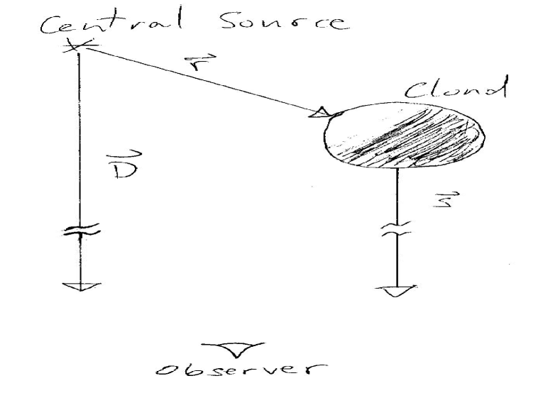
Figure 2.1: Definitions of ${\bf D}$, ${\bf r}$, and ${\bf s}$.

Figure 2.1). Here we take ${\bf\hat{s}}$ as the unit vector of ${\bf s}$. As will be discussed in § 3.1, $L_{l*}$ depends upon the position of the star and time-dependent luminosity of the central source $L$. The line profile $F_{l}(t,v_{\rm D})$ is the contribution to the line flux by the objects that have a line-of-sight velocity $v_{\rm D}$. As shown in Blandford & McKee (1982), for example, this profile can be expressed as

$$F_{l}(t,v_{\rm D})=\int d^{3}rd^{3}v{L_{l*}(t-s/c,{\bf r,\hat{s}})\over 4\pi s^{2}}f\delta(v_{\rm D}+{\bf v\cdot\hat{s}}),$$ (2.1)

where ${\bf v}$ is the cloud velocity vector and $f$ is the stellar phase space distribution function. In the above equation, the delta function in velocity serves to select the clouds with line-of-sight velocity $v_{\rm D}$ under the simplifying assumption that we can ignore the intrinsic line widths of the clouds.

Strictly speaking, equation (2.1) is only valid under special conditions. For instance, as discussed in Appendix G, the cloud equilibrium times must be much less than the times for clouds to traverse the line-emitting region. As shown in Appendix G, the cloud crossing times are generally more than a year, so this assumption is probably valid for many models. A more questionable assumption of equation (2.1) is that the line emissions from the clouds do not have any explicit dependences upon the directions of the velocity vectors. The validity of this assumption is discussed in Appendix L. Another assumption of equation (2.1) is that the number of clouds must be much larger than a fraction of the ratio of the entire line width to the line widths of the individual clouds. This is so that the emitted line profiles are smooth (in accordance with observations). As discussed in § 1.3, this assumption appears to be reasonable in emission, at least for most of our models. For reasons discussed in Appendix K, however, it is probably invalid in absorption. In fact, equation (2.1) is inapplicable for systems with significant BLR line or continuum absorption. In the spirit of simplicity, and because we are primarily interested in just the emission characteristics, we will hereafter assume that each of these conditions is met.

We also assume that $f$ is not an explicit function of the velocity vector ${\bf v}$. Specifically, we assume that $f$ and $L_{l*}$ are the same on the $\theta_{v}=\cos^{-1}(v_{\rm D}/v)$ and $\theta_{v}=\pi-\cos^{-1}(v_{\rm D}/v)$ cones of velocity phase space. As a result, the profiles and their responses of our AGN wind models are symmetric in velocity space. These assumptions permit the delta function in equation (2.1) to remove the remaining integration over velocity. The time-averaged line profile thus becomes simply an integration over the number density of the reprocessing objects.

2.2 The Linearized Response Functions

As mentioned earlier in this and the previous chapter, most AGN line emission models consist of a point continuum source that ionizes the surrounding clouds. These clouds then respond to changes in the ionizing flux through changes in the associated line emission. Since the continuum sources in AGN are highly time-dependent, these models predict that the line emission should also be time-dependent. However, since it is believed that these clouds are located at distances much larger than the size of the continuum source, the lines should be delayed compared to continuum flux. These delays can then be used to probe the distribution and radially dependent properties of the line-emitting clouds.

If the system responds linearly, the time-dependent luminosity emitted in line $l$ can be written as an integral over the time history of the continuum source luminosity (e.g., Blandford & McKee 1982):

$$F_{l}(t)=\int_{0}^{\infty}dt^{\prime}L(t-t^{\prime})\Psi_{l}(t^{\prime}).$$ (2.2)

In this equation, $\Psi_{l}$ denotes the response function of the system. In the linear regime it indicates the response in time to an impulsive input at $t=0$. As discussed in the previous subsection, variability in the luminosity of the continuum source results in variation of the total line flux; equation (2.2) provides a means of calculating the response of the system to changes in the continuum as a function of both the time and the velocity across the line profile, i.e. to compute the time-dependent line emission flux given the history of the continuum light curve.

The procedure employing response functions has also been called “echo mapping.” This is because it is similar to the procedure used with sonar and other active measurement systems. With sonar, the input is a “ping” given off by a submarine, for instance. The delay of the echo from this ping provides the distance of nearby underwater objects. If there are enough objects underwater, the echo is a smooth function. This is the response function. However, in an AGN there are no well-defined pings. Rather, there is only a smooth time-dependent continuum light curve. Provided the system is linear and one has obtained enough data, the response function obtained upon deconvolution of the data is unique and the same that would be obtained if AGNs pinged. In this linear case, an analysis of line and continuum light curves could be used to constrain the spatial distribution of clouds around the black hole. For instance, as shown in Appendix F, an optically thin spherically distributed shell of linearly responding clouds would have a hat-shaped response function.

There are, however, indications that AGN systems are nonlinear (e.g., Kinney et al. 1990, Maoz 1992). Because most AGN line emission models predict nonlinear line emissivity and cloud area functions, this nonlinearity is actually what one would expect. In the nonlinear case, linear response functions do not represent the system well. In particular, even with a hypothetical infinite quantity of error-free data, the response functions obtained upon deconvolution would be highly dependent upon the shape of the continuum light curve in the data set.

To avoid this problem, one could resort to fully nonlinear model fitting. Unfortunately, as discussed in Appendix F, this would be very computationally expensive.

As an alternative to abandoning response functions altogether, one can simply include the next term in the Taylor expansion of the nonlinear response. The procedure for doing this is described in detail in Appendix H. This leads to the introduction of the following additional parameters: the average of the input, the average of the output, and the “gain” of the output. The gain of the flux of a line is defined as its logarithmic derivative with respect to the continuum flux. It simply tells the extent to which the system is nonlinear. Thus, a system with gain of unity acts linearly, for example, while a system with a gain of 2 has an output response amplitude that is twice that of the amplitude input to the system.

Equation (2.2) modified to include these extra parameters becomes

$$F_{l}(t)=<F_{l}>\left(1+\int_{0}^{\infty}dt^{\prime}\left[{L(t-t^{\prime})\over<L>}-1\right]{\hat{\Psi}_{l}}(t^{\prime})\right).$$ (2.3)

In this equation and throughout this dissertation, $<x>$ represents the average over the entire data set of quantity $x$. The new input for the system the above equation represents is the expression in square brackets, which is simply the fractional fluctuation of the continuum about the mean. We have used the symbol “$\bigwedge$” above $\Psi_{l}$ to indicate two things:

1. That we are dealing with the first order in the Taylor expansion of a nonlinear system rather than a truly linear system. The output of a linear system is proportional to the input. Because of the term of unity in equation (2.3), this does not occur. However, it does occur if the $\bigwedge$’ed variables are taken as the actual input and output of the system. Thus, for the $\bigwedge$’ed variables, the analysis is fully linear. We hereafter adopt the term “linearized” to denote the transformation of variables to their deviations about their means such that tools like equation (2.2) can be employed.

2. That we are using a “normalization-independent” response function with units of inverse time, such that the transfer function (which is just the Fourier transform of the response function) and gain are dimensionless. We will, however, adhere to the standard convention that the “$\bigwedge$” symbol denotes only the unit vector when it is above a vector.

The normalization-independent response function in equation (2.3) can also be obtained by applying the procedure described in described in Appendix H. Applying this procedure to equation (2.1) yields

$${\hat{\Psi}_{l}(t)}=\int d^{3}rd^{3}v{<L_{l*}(t,{\bf{r,\hat{s}}})>\over<L>4\pi s^{2}}\left\{\eta(L_{l*}|L)\delta\left(t-{{\bf{r}}\over c}\cdot({\bf{\hat{r}-\hat{D}}})\right)\right\}f.$$ (2.4)

This equation is used to obtain the response functions shown in Chapter 4. The bracketed factor is the linearized response function of an individual cloud due to variations in the observed continuum luminosity. The factor of $\eta(L_{l*}|L)$ is the asymptotic gain of an individual stellar wind line flux $L_{l*}$ due to small variations in the continuum luminosity $L$ about its local average. The asymptotic gain is the normalization-independent transfer function at an excitation frequency of zero. This gain is dependent upon the local continuum flux (among other things), which is of course position-dependent.

Strictly speaking, equation (2.4) is merely the spatial response function. If the cloud equilibrium times are comparable to the light crossing times, the response function of the system is the convolution of the spatial response function with the local response functions of the clouds. For simplicity, we will hereafter make the “fast cloud” assumption, which is that the local response functions are delta functions in lag, i.e., that the local response time is much less than the light crossing time. In other words, we assume that we can ignore the details of the time-dependent responses of the clouds and concern ourselves only with the asymptotic gains of their line emission fluxes. The validity of this assumption is discussed in Appendix F. This assumption yields fewer parameters because any frequency dependence of the cloud gains is ignored; only the asymptotic gains are employed.

The beauty of the above expansions is that, for a given nonlinear model and continuum average, we can now fully compute the response function that would be obtained for hypothetical infinitesimal continuum variations. Unlike the fully linear response function, this “linearized” response function is unique for a given nonlinear model and average continuum. Moreover, it yields the important physical information about the positions of the clouds in the nonlinear system. The main drawback is that it cannot tell us the absolute number of clouds along the iso-delay surface, but rather only the number relative to the other clouds in the system.

One complexity of our model is its very large spatial extent. This yields an extended tail in the response functions. Study of response function tails is systematically difficult because the duration of such monitoring campaigns must be several times that of the light travel time of the region one intends to probe. The recent AGN monitoring campaigns, lasting only a month or so, may have only probed a small fraction of the nonzero response function of the system. Because our model is well defined across its entire spatial extent, we are able to use equation (2.4) to compute the response function at arbitrarily large time delays.

2.3 The Velocity-Resolved Linearized Response Functions

In the previous subsection, we obtained the profile-integrated response functions for nonlinear models. With the higher resolution data recently made available, we can also accurately measure time-dependent line profile shapes. In order to employ this data to constrain models, we can simply extend the results of the previous subsection into velocity/wavelength space.

The velocity-resolved normalization-independent response function is just

$${\hat{\Psi}_{l}(t,v_{\rm D})}=\int d^{3}rd^{3}v\frac{<L_{l*}(t,{\bf{r,\hat{s}}})>}{<L>4\pi s^{2}}\left\{\eta(L_{l*}|L)\delta\left(t-{{\bf{r}}\over c}\cdot({\bf{{\hat{r}}-{\hat{D}}}})\right)\right\}f\delta(v_{\rm D}+{\bf{v\cdot{\hat{D}}}}).$$ (2.5)

This equation gives the response of the cloud system to changes in the continuum flux at a specific velocity $v_{\rm D}$. It is different from equation (2.4) only by the addition of a delta function in Velocity. This delta function isolates just the clouds moving at a line-of-sight velocity $v_{\rm D}$. We employ this equation to produce the velocity-resolved response functions shown in Chapter 4.

Chapter 3 Approximations for the Cloud Luminosity $L_{l*}$ and the Distribution Function $f$

In Chapter 2 we showed general expressions of the line profiles and response functions associated with a generic system of “clouds” which reprocess continuum radiation into lines. The details of the model are contained in the precise forms of the apparent line luminosity per reprocessing object $L_{l*}$ and the distribution function of reprocessing objects $f$. In this chapter, we discuss the assumptions and methods we used in calculating these quantities for the models presented in Chapter 4.

3.1 Approximations of the Cloud Luminosity $L_{l*}$

We assume that the angular distribution of the continuum radiation is isotropic and that there is no intervening absorption. However, as we shall see shortly, the mean column densities of the clouds can be very high. We, therefore, do not assume that they emit isotropically. An expression compatible with these assumptions for the apparent line luminosity of an individual reprocessing stellar wind for an observer at ${\bf{D}}\equiv{\bf{r+s}}$ is

$$L_{l*}(t,{\bf{r,\hat{s}}})={L\over 4\pi r^{2}}A\epsilon_{l}(1+\epsilon_{{\rm{A}}l}\bf{\hat{r}}\cdot{\bf{\hat{s}}}).$$ (3.1)

In the above equation, $A$ is the area per cloud (which in general depends on the time-retarded continuum luminosity and the position of the cloud), $\epsilon_{l}$ is the efficiency for converting continuum into line radiation, and $-1\leq\epsilon_{{\rm{A}}l}\mathrel{\hbox{\hbox to0.0pt{\hbox{\lower 5.0pt\hbox{$\sim$}}\hss}\hbox{$<$}}}0$ is the line-dependent anisotropy factor, also called the beaming factor. The anisotropy factor, which incidentally has nothing to do with the wind area, accounts in a simple fashion for the line emission that is beamed back towards the continuum source. Such beaming is especially important for lines in which the clouds are very optically thick, such as Ly$\alpha$. According to this prescription, such a line would have $\epsilon_{{\rm{A}}l}\simeq-1$. In this case, equations (2.4) and (2.5) would yield a response function that is proportional to the time lag $\tau$ for small enough values of $\tau$. Such a response function would therefore be equal to zero at $\tau=0$. This would occur because the clouds that would be both nearest to the observer and along the zero-delay line of sight towards the observer would emit all of their line emission back towards the continuum source. Conversely, if $\epsilon_{{\rm{A}}l}\simeq 0$, the response function would, at least for simple geometries, be a monotonically decreasing function of lag.

Linearization of equation (3.1) yields (see eq. [F.6])

$$\eta(L_{l*}|L)=1+\eta(A|L)+\eta(\epsilon_{l}|L)+\frac{<\epsilon_{{\rm A}l}>\bf{\hat{r}}\cdot{\bf{\hat{s}}}}{1+<\epsilon_{{\rm A}l}>\bf{\hat{r}}\cdot{\bf{\hat{s}}}}\eta(\epsilon_{{\rm A}l}|L).$$ (3.2)

The second and third terms of this equation are discussed, respectively, in § 3.1.1 and § 3.1.2. Because the column densities are so high for nearly all of the models we compute, $\epsilon_{{\rm A}l}$ is insensitive to the continuum flux and $\eta(\epsilon_{{\rm A}l}|L)$ is negligible. In our calculations we therefore ignore the last (fourth) term of this equation.

Equation (3.1) states that the line emission from a wind is dependent upon the cloud area $A$, the line efficiency $\epsilon_{l}$, and the anisotropy factor $\epsilon_{{\rm{A}}l}$. In the following, we discuss in turn the assumptions and approximations made for each of these functions.

3.1.1 Approximations for the Cloud Area $A$

Following Kazanas (1989), we assume that the cooler stars such as the red giants have winds that slowly emanate from the stars. The properties of an individual wind are a strong function of the value of the local continuum flux to which it is exposed. Since the luminosity of a given AGN varies much less than $r^{-2}$ (a factor of $\sim 2$ verses a factor of $\sim$100), these wind characteristics are primarily a function of the distance from the black hole. There are at least four different regions interest:

• A region in which the winds are optically thick to the UV continuum. The winds terminate at distances from the red giants where the ionization parameters at the wind edges would be greater than $\Xi^{*}_{\rm{c}}$. In this dissertation, $\Xi\equiv F_{{\rm c}}/cP$ (where $F_{{\rm c}}$ is the normal component of the local continuum flux vector between 1 and 1000 Ry and $P$ is the gas pressure at the wind edge) is the pressure ionization parameter and $\Xi^{*}_{\rm{c}}$ is the critical pressure ionization parameter in Krolik, McKee, & Tarter (1981) above which the temperature rises to the “hot phase” of $T\sim$10⁸ K. As a result of this wind edge condition, the effective area of the reprocessing portion of a cloud $A$ decreases with increasing local continuum flux. In particular, Kazanas (1989) obtained for clouds in this region

  $$R_{\rm{w}}\simeq 7\times 10^{13}r_{17}\left(\frac{\dot{M}_{-6}}{v_{\infty 10}L_{44}}\right)^{1/2}\,\textrm{cm},$$ (3.3)

  where $r_{17}$ is the distance to the cloud in units of $10^{17}$ cm, ${M}_{-6}$ is the wind mass loss in units of $10^{-6}$ $M_{\odot}$ per year, $v_{\infty 10}$ is the wind terminal velocity in units of 10 km s^-1, and $L_{44}$ is the bolometric continuum luminosity measured in $10^{44}$ erg s^-1, which is a typical luminosity for the Seyfert class of AGNs.

• A region where the clouds are optically thin to UV continuum radiation. The above functions yield a cloud size to ionizing region fraction of $R_{\rm w}/d_{\rm{S}}\propto N_{\rm c}/\Xi\propto(L/r^{2})^{-1/2}$, where $d_{\rm{S}}$ is the depth of the inverse Strömgren region and $N_{\rm c}$ is the column density. Thus, the clouds are recombination-limited and optically thin to UV continuum radiation at large enough distances from the black hole. In this second possible region, the wind boundary conditions are less important, and the effective area shrinks down to the cross-sectional area of the inverse Strömgren region, which is straightforward to calculate. The result is $A_{\rm eff}\propto(L/r^{2})^{-2/3}$ for the clouds in this distant region, where $A_{\rm eff}$ denotes an effective area different from the physical wind area $A$. This area function maintains a constant $N_{\rm c}/\Xi$, where the cloud edge parameters now represent an average over the line-emitting section of the wind. Both of the area expressions for these first two possible regions are approximations to the one obtained upon introducing an upper cutoff to the integral in equation (4) of Scoville & Norman (1988).

• A region very near to the black hole in which the stellar winds are approximately the same sizes as the photospheres. This region exists because the winds can become fully “stripped” if the local continuum flux is high enough.

• A region of low column density clouds far from the black hole. Far enough from the black hole, the mean column density associated with the cool region of the winds decreases at least as fast as $r^{-2/3}$. Thus, as the distance from the continuum source increases, the mean column density would decrease without limit as the winds became arbitrarily large and tenuous. Though the wind cloud model does not “need” an external hot medium to pressure confine the clouds, such a medium is bound to exist, and in certain models is even necessary to fuel the continuum source. Because the stars are accelerated by the black hole to extremely high speeds and the intercloud medium is probably stationary, ram pressure must affect the more tenuous elements of the wind. As discussed in Appendix E, this is important for high enough values of the inter-cloud density. We do not attempt a detailed calculation accounting for such effects, as it would be beyond the scope of this dissertation. We do, however, impose upper limits to the sizes of the clouds in the models by employing a free parameter $N_{\rm cmin}$ to denote the minimum permissible mean column density. By adjusting this parameter, we are able to avoid models with winds that would be unrealistically large and tenuous. In this fourth and final possible region, we therefore assume $N_{\rm c}=N_{\rm cmin}$.

In practice, we calculate the line emission from the actual column densities of the geometrical wind and do not use the effective area function $A_{\rm eff}$. For almost all of the models we calculate, $N_{\rm cmin}$ is high enough that the outermost region in which the winds are optically thin is never actually realized, especially where the covering is substantial. Thus, the errors introduced by ignoring the high-pressure region associated with $A_{\rm eff}$ are probably small. As a result, most of our models have at most only three, successively more distant regions with at most two boundaries. We denote these two boundaries by the parameters $r_{12}$ and $r_{23}$.

In the simplest case, the cloud properties at these three boundaries would be non-differentiable, with their radial dependences changing suddenly. This would result in discontinuous gains. It is unlikely, however, that the stars in AGNs are identical. Thus, in more realistic models with several different stellar types, the actual boundaries would probably be smooth without any discontinuities. To account for this, our gain computer code smoothes the relevant properties of clouds located near a boundary.

While we assume spherical symmetry in calculating the radius and particle density of the wind, we attempt to account for suspected asymmetry due to continuum radiation pressure. We do this by increasing the final area by a factor of four (Kazanas 1989).

In Kazanas (1989), the radial velocity of the winds was assumed to be independent of the distance from the stellar surface. In this paper, we attempt a more accurate analysis. We assume that the wind velocity $v$ as a function of the distance $R$ from the center of the star is

$$v(R)=v_{\infty}\left(1-{R_{*}\over R}\right)^{-1/2},$$ (3.4)

where $R_{*}$ is the radius of the red giant, which is $1.5\times 10^{13}$ cm for the models presented here. For most of our models $R_{\rm w}\gg R_{*}$ and the particular exponent of equation (3.4) (assumed in our work to be -1/2) is not particularly important. This is because the form of equation (3.4) yields a sudden decrease in the wind velocity near the surface of the star. Since we assume

$$\dot{M}=4\pi R^{2}v\rho,$$

where $\rho$ is the mass density of the wind, the pressure of the wind is a steep function of $R$ only for $R\sim R_{*}$. The ionized, line-emitting, inverse Strömgren region is much smaller than $R$ in most of our models, so even iso-velocity wind models yield similar results. The exceptions to this occur at very high fluxes (very near to the continuum source) in our models without mass loss enhancement. In this situation, ionization parameters as low as $\Xi^{*}_{\rm{c}}$ are only obtained at very high densities very close to the stellar surface. This results in $R_{\rm w}\simeq R_{*}$ independent of the precise value of the very high local continuum flux. In other words, $R_{*}$ is a lower limit to the effective size of the line-emitting area of the stellar wind.

Under the above assumptions, the functional dependence of the line-emitting cross-sectional area of the wind upon the local continuum flux level is straightforward to calculate. This area is shown for model 1 in

Figure 3.1: Solid thin line, left vertical axis: wind area $A$ as a function of distance from the black hole $r$ (horizontal axis) for model 1. Solid thick line, right vertical axis: the pressure $P$ at the wind edge.

Figure 3.1. The bolometric luminosity of model 1 is $1.0\times 10^{44}$ ergs s^-1. All other parameters of model 1 are the same as the fiducial ones assumed in Kazanas (1989). Specifically, the wind edge ionization parameter is $\Xi=10$, the giant star mass loss rate is $\dot{M}=10^{-6}\,M_{\odot}$ yr^-1, and the terminal wind velocity is $v_{\infty}=10$ km s^-1. Note that near the black hole (at relatively high values of the local continuum flux), the area is essentially the size of the stellar envelope. Conversely, far away from the black hole (at relatively low values of the local continuum flux), the area attains its upper limit in size. For this model, $N_{\rm{cmin}}=8\times 10^{21}$ cm^-2, which yields a maximum wind cross-sectional area of $4.8\times 10^{-7}$ pc² ($4.6\times 10^{30}$ cm²).

Though the above parameters define the cloud area function of model 1, some of their values are now questionable. For instance, Kazanas (1989) assumed $\Xi=\Xi^{*}_{\rm c}=10$ for the outer edge of the cool zone for all winds; the ionization parameter was independent of the local continuum flux and the edge pressure obeyed $P\propto(L/r^{2})^{1.0}$. However, near the wind edge boundary there is a strong temperature and ionization gradient which defines the conduction zone between hot and cool plasma. In the pressure-equilibrium model, these regions are assumed to be in pressure equilibrium. Because of the difficulties that would be involved, essentially all computations of line emission from pressure-equilibrium clouds ignore this relatively high ionization region. One difficulty is that the plasma in the conduction zone would not even be in static equilibrium; because line cooling becomes unimportant at high enough temperatures and ionization parameters, this plasma would be heated up to the Compton temperature on the thermal instability time scale. This time scale is inversely proportional to the position-dependent difference between the heating and cooling rates from photoionization, Compton scattering, line emission, and thermal Bremsstrahlung. This position-dependent heating rate function in turn would depend upon the structure of the local temperature and ionization parameter functions in the conduction zone. The precise ionization parameter to impose at the cool edge of our simple models in order to best account for the conduction zone and the evaporation within it is not clear to us. However, near and above the Krolik, McKee, & Tarter (1981) $\Xi=\Xi_{\rm{c}}^{*}\simeq 10$ limit, the thermal instability is very strong. Therefore, plasma with ionization parameters near this limit should rapidly evaporate and be physically thin. For this reason, the value of the ionization parameter at the edge of the cool zone which best approximates the complex situation is probably much smaller than this. In the stellar wind case of interest here, the evaporation is balanced by mass loss rate (as in eq. [1.7]) and pressure equilibrium is not required. Thus, for the case of interest here, the location the conduction zone and the ionization parameter at the cloud edge are additionally a function of the mass loss rate. In contrast, the two-phase, pressure-equilibrium clouds, which have no reservoir of cool gas, eventually would evaporate completely (Krinsky & Puetter 1992).

To account for the required thinness of any high ionization layers on the clouds, Taylor (1994) assumed that the location of the wind edge cannot be in equilibrium if the efficiency of C IV (one of the most important cooling lines) has a gain of less than -1.0 due to changes in the ionization parameter. With this assumption, the first and third terms in equation (3.2) cancel each another for models in which $P\propto L/r^{2}$. A side benefit of doing this was that it resulted in asymptotic gains of Ly$\alpha$ and C IV that agree with the observations by Krolik et al. (1991) that indicate, among other things, an intrinsic Baldwin effect in NGC 5548.

In this dissertation, we make no such attempt to compute the precise location and ionizational structure of the conduction zone. We do, however, attempt to account for the possibility of flux-dependent edge conditions by considering models in which $P\propto(L/r^{2})^{s/2}$, where $s$ is a free parameter. This prescription is slightly different from that of Rees, Netzer, & Ferland (1989), who assumed the cloud pressures scale with distance according to $P\propto r^{-s}$. Rees, Netzer, & Ferland (1989), however, did not compute response functions. Thus, in that paper it was irrelevant as to whether the cloud pressure in their models was a direct function of position or merely an indirect function via the radial dependence of the local continuum flux. In the models shown in Chapter 4, we assume the latter.

An additional assumption in question concerns the mass loss. It has been suggested that the AGN continuum is strong enough to influence some of the cooler stars in the vicinity of the continuum source (e.g., Edwards 1980, Penston 1988, Norman & Scoville 1988, Tout et al. 1989; cf Voit & Shull 1988). Problems with this assumption are discussed in § 1.2.7. A detailed analysis of the effect of continuum heating upon the structure of stellar winds is beyond the scope of our work. Nevertheless, for completeness we also compute models which follow the prescription of Norman & Scoville (1988), who suggested that the mass loss rate per star would be a function of position, with $\dot{M}\propto r^{\delta}$. We assume a luminosity dependence and adopt $\dot{M}\propto(L/r^{2})^{\alpha(r)}$, where the radial dependence in $\alpha(r)$ is only employed to prevent $\dot{M}<\dot{M}_{\rm min}$, where $\dot{M}_{\rm min}$ is the mass loss of stars outside of the line-emitting region. The addition of the $\alpha$ parameter permits us to consider models somewhat different from that of Kazanas (1989). If $\alpha>0$, the effective area is a weaker function of the local continuum flux than if $\alpha=0$. For this reason, $r_{12}$ and $r_{23}$ can be undefined for some $\alpha>0$ models. For models with winds that are radiatively excited, one expects $\alpha\sim 1$ (§ 1.2.7).

Employing the above parameters yields an asymptotic area gain (which, as before, is simply $d\textrm{ln}A/d\textrm{ln}L$) of

$$\eta(A|L)=\left\{\begin{array}[]{cc}0&r\mathrel{\hbox{\hbox to0.0pt{\hbox{\lower 5.0pt\hbox{$\sim$}}\hss}\hbox{$<$}}}r_{12}\\ \alpha(r)-s/2&r_{12}\mathrel{\hbox{\hbox to0.0pt{\hbox{\lower 5.0pt\hbox{$\sim$}}\hss}\hbox{$<$}}}r\mathrel{\hbox{\hbox to0.0pt{\hbox{\lower 5.0pt\hbox{$\sim$}}\hss}\hbox{$<$}}}r_{23}\\ 0&r\mathrel{\hbox{\hbox to0.0pt{\hbox{\lower 5.0pt\hbox{$\sim$}}\hss}\hbox{$>$}}}r_{23}\end{array},\right.$$ (3.5)

where, as discussed in the beginning of this subsection, $r_{12}$ and $r_{23}$ denote the boundaries between the “bleached,” optically thick, and column density-limited regions. Equations (3.2) and (3.5) are used to compute the linearized response functions that are shown in Chapter 4 for our models. For comparison, the parameters in Kazanas (1989) yield $\eta(A|L)=-1.0$.

3.1.2 Approximations for the Line Efficiencies $\epsilon_{l}$ and the Anisotropy Factors $\epsilon_{{\rm{A}}l}$

Equation (3.1) for the cloud line luminosity $L_{l*}$ also contains the line efficiencies $\epsilon_{l}$ and the anisotropy factors $\epsilon_{{\rm{A}}l}$. The line efficiency of a stellar wind is harder to compute than the efficiency of a traditional cloud such as the ones considered by Kwan & Krolik (1979). This is partly because the fundamental properties of the line emitting gas within a wind can be a function of the “impact parameter” $p$, which is defined to be the perpendicular distance from the radius vector ${\bf r}$ that extends from the black hole to the star. In Alexander & Netzer (1994), the line efficiency was calculated by partitioning the clouds/winds into shells of various impact parameters. One-dimensional radiative transfer was then applied to each shell.

Our approach in determining $\epsilon_{l}$ is more modest; we merely partition each wind of cross-sectional area $A$ into two sections of equal area: a “face-on region” and an “angled region.” The face-on region represents the inner cylindrically shaped region of a cloud with low impact parameters. This region is assumed to have a pressure at the edge of the cloud of $P=F/(c\Xi)$, where $c$ is the speed of light and $F$ is simply $L/(4\pi r^{2})$ rather than the slightly more complicated normal component of the flux vector. The angled region represents the outer portions of the wind that have higher impact parameters. In the angled region, the normals of the tangential surfaces of the wind edge are not parallel to the continuum flux, but are rather offset by a mean angle of $\theta$. We assume that the edge pressure in this region is $P=F/(c\Xi\cos\theta)$, which should be valid for optically thick winds. We then simply adopt $\theta=\pi/4$.

For this prescription to be accurate, the size of the ionized, line-emitting, inverse Strömgren region must be much smaller than the size of the winds. In other words, as stated above, the winds must be highly optically thick to most of the continuum. In this case, line emission occurs from only a thin (relative to the scaling size of the pressure gradient) outer skin, and only the edge conditions (including the incidence angle of the flux with respect to the normal of the wind surface $\theta$) are important. (Conversely, if a significant portion of a wind is optically thin, the edge conditions become relatively unimportant.) Assuming the size of the ionized region is approximately $d_{{\rm Ly}\alpha}\simeq F_{\rm c}/(\textrm{Ry}\cdot n_{\rm H}\alpha_{\rm B})$ (where $n_{\rm H}$ is hydrogen density, $\alpha_{B}$ is the Menzel-Baker case B hydrogen recombination coefficient, and 1.0 Ry=13.6 eV), the winds become thin when the column density to ionization parameter ratio $N_{\rm c}/\Xi$ exceeds $\simeq 10^{22}$ cm^-2. In

Figure 3.2: Solid line, left axis: the mean column density as a function of radius from the continuum source $r$ (horizontal axis) for model 1. In the broad line region, the column density drops off faster than 1/$r$ because the radial velocity of these winds at the edge is significantly less than the terminal velocity. Dotted line, right axis: the ionization parameter $\Xi$. For this model, the ionization parameter is constant throughout most of the broad line region with $\Xi=\Xi^{*}_{\rm{c}}\simeq 10$. Beyond $0.15$pc, the mean column density reaches its minimum permitted value, the edge pressure becomes independent of $r,$ and the effective ionization parameter is assumed to be inversely proportional to the local continuum flux.

Figure 3.2, the mean column density and ionization parameter of the winds for model 1 are shown. The column density to ionization parameter ratio is generally above 10²³ cm^-2, especially in the broad line region. Therefore, calculations accounting for pressure gradients within clouds are probably not necessary for most of the regimes of parameter space we are concerned with, and our approximations should be valid.

We, therefore, treat the two regions of the cloud as being independent and assume that the line efficiency of each region is a simple function of only the edge conditions (e.g., the pressure and ionization parameter) and the column density, which we assume is less in the angled region by a factor of $\sqrt{2}$. The line efficiency of each region was calculated via three-dimensional interpolation of results obtained using the radiative transfer code XSTAR version 1.20 (e.g., Kallman 1995). The grid we constructed was large; the ionization parameter, pressure, and column density were calculated, respectively, at 10, 6, and 6 values (for a total of 360 node points). In accordance with the edge conditions being regulated by the ionization parameter (rather than the density), we assumed the pressure is constant throughout each region.

Unlike line profiles, linearized response functions contain a factor of the line emissivity gain $d\textrm{ln}L_{l*}/d\textrm{ln}L$ (e.g., Goad et al. 1993, Taylor 1996). Because the expression for the gain contains derivatives of the emissivity and because the resolution of the grid we used was so high, the calculated gain was very sensitive to the systematic error in the calculated line emissivity. In order to obtain gains that did not have numerous discontinuities, we modified the step size routine of XSTAR. XSTAR normally calculates the step sizes such that changes in continuum optical depth at each energy is at most 1.0 from one slab to the next. The routine we used is simpler, yet is more computationally expensive. It sets the step size within each region to be inversely proportional to the heating rate in the previously calculated zone. This increases the number of steps taken near the cloud “face” and decreases the number of steps taken in the cooler (and less energetically important) portions of the clouds. The actual number of steps within each cloud was then adjusted such that the flux from each of the 32 spectral regions that were calculated deviated by 5% or less from a run at much higher resolution. For ionization parameters above $\sim 1$, the modified step routine affects some of the high ionization lines, such as He II $\lambda$1640 Å and N V $\lambda$1243 Å. In addition, the modified routine yields smoother line emissivity functions (as determined from viewing two-dimensional cuts of their three-dimensional structure) and relatively continuous gains. This may be due to the relative insensitivity of our step routine to highly position-dependent continuum opacities at high ionization parameters (which might be caused by, for instance, the He II $\lambda 228$ Å  (54 eV) absorption edge).

XSTAR was also used to obtain the anisotropy factor $\epsilon_{{\rm{A}}l}$ of each region. For simplicity, we assume the angled region has the same anisotropy factor as the face-on region. Because of the very high column densities we assumed, we found $\epsilon_{{\rm{A}}l}\sim-1$ for most of the lines and regimes of parameter space we explored.

In Kazanas (1989), the ionization parameter at the edge of the clouds $\Xi$ was fixed, so the asymptotic gain of the line emissivity due to variations in the continuum $\eta(\epsilon_{l}|L)$ was simply $\eta(\epsilon_{l}|P)$. In other words, only the dependence of the emissivity upon the pressure affected the line ratios. Employing the more general parameterization described in § 3.1.1, this becomes

$$\eta(\epsilon_{l}|L)=\left\{\begin{array}[]{cc}\eta(\epsilon_{l}|P)(1-\frac{s}{2})\eta(\epsilon_{l}|\Xi)+\frac{s}{2}\eta(\epsilon_{l}|P)+\frac{1}{2}\left(\alpha(r)+\frac{s}{2}\right)\eta(\epsilon_{l}|N_{\rm c})&r\mathrel{\hbox{\hbox to0.0pt{\hbox{\lower 5.0pt\hbox{$\sim$}}\hss}\hbox{$<$}}}r_{23}\\ \eta(\epsilon_{l}|\Xi)&r\mathrel{\hbox{\hbox to0.0pt{\hbox{\lower 5.0pt\hbox{$\sim$}}\hss}\hbox{$>$}}}r_{23}\end{array}.\right.$$

The upper expression above is valid for winds near the continuum source at $r\mathrel{\hbox{\hbox to0.0pt{\hbox{\lower 5.0pt\hbox{$\sim$}}\hss}\hbox{$<$}}}r_{23}$. Without any mass loss enhancement, these winds would shrink when the continuum brightens to maintain a relatively constant ionization parameter (assuming $s>0$). The lower expression is valid for winds that are optically thin or that have a truncated column density. For nearly all of the models we calculate, the third, right-most term in the upper expression for the $r\mathrel{\hbox{\hbox to0.0pt{\hbox{\lower 5.0pt\hbox{$\sim$}}\hss}\hbox{$<$}}}r_{23}$ region is approximately an order of magnitude smaller than the first two terms. This is because the column densities of our models are so high. We therefore ignore this term in our calculations. Standard interpolation algorithms were used to solve the other terms. As mentioned in § 3.1.1, we smoothed $\eta(\epsilon_{l}|L)$ near the $r_{23}$ boundary to prevent unphysical discontinuities in $\eta(\epsilon_{l}|L)$ as well as to avoid potential numerical complications.

3.2 Approximations for the Phase-Space Distribution Function $f$

In addition to $L_{l*}$, knowledge of the cloud phase space distribution function $f$ is necessary in order to determine the line profiles (eq. [2.1]) and response functions (eqs. [2.4] & [2.5]) of the models under consideration. In this subsection we discuss $f$ and our assumptions about it.

The stellar distribution functions in AGNs are not well known. One might hope to try to base the stellar distribution functions upon available observations. Unfortunately, the measurement of the distribution function in real systems is difficult since one measures only moments of it, such as the surface brightness profile. From this, one can infer the density as a function of radius. The velocity information that does exist for some systems which are thought to harbor “dead” black holes at their centers is usually just the velocity dispersion alone, which is not sufficient to provide the stellar distribution function but rather only imposes quantitative constraints on it. For galaxies which contain active nuclei, such measurements are very difficult since the emission near the center is dominated by the point-like source of the continuum.

Fortunately, if we assume that the clusters are in steady state in most regions, we can employ the Jeans theorem. This states that distribution functions of such systems are dependent only upon integration constants of the equations of motion, such as the angular momentum and energy per unit mass

$$E=\phi(r)+\frac{v^{2}}{2}\mathrel{\hbox{\hbox to0.0pt{\hbox{\lower 5.0pt\hbox{$\sim$}}\hss}\hbox{$<$}}}0.$$ (3.6)

In this equation, $\phi$ is the gravitational potential. If we assume that the entire system (in which the supergiants constitute a small fraction of the total mass) is spherically symmetric, then this gravitational potential is

$$\phi(r)=-\left\{\frac{GM_{\rm h}}{r}+4\pi GM_{\rm{rat}}\left({1\over r}\int^{r}_{0}dr^{\prime}n_{*}(r^{\prime})r^{\prime 2}+\int^{\infty}_{r}dr^{\prime}n_{*}(r^{\prime})r^{\prime}\right)\right\},$$ (3.7)

where $M_{\rm h}$ is the mass of the supermassive black hole and $M_{\rm{rat}}$ is the mass density divided by the giant star number density $n_{*}$. For simplicity, we assume here that $M_{\rm rat}$ is independent of radius. This assumption is clearly not ideal; in the models of Murphy, Cohn, & Durisen (1991), the density functions have a strong mass and radial dependence, especially for $r_{\rm t}\ll r\ll r_{\rm c}$ (where, as before, $r_{\rm t}$ is the tidal radius and $r_{\rm c}$ is the core or gravitational radius of the system). However, this assumption has an important feature of permitting the distribution function to be determined purely from the surface brightness functions. These surface brightness functions have been measured in nearby galactic nuclei, though only for $r\mathrel{\hbox{\hbox to0.0pt{\hbox{\lower 5.0pt\hbox{$\sim$}}\hss}\hbox{$>$}}}0.1$ pc.

Inside $r\sim 0.1$ pc, constraints upon $f\textrm{ }$ can be imposed by employing theoretical results, such as those obtained with Murphy, Cohn, & Durisen’s Fokker-Plank code. Note that their models are highly input dependent for the densities beyond about one parsec, where the stars do not interact fast enough to be independent of the somewhat arbitrary initial distribution that was assumed. On the other hand, their results for radial distances less than a parsec show that collisions become important when the stellar density is above $\sim 10^{7}$ M_⊙ pc^-3. Murphy, Cohn, & Durisen (1991) assumed that tidal disruption imposes the boundary condition that the density of giant stars $n_{*}(r)$ is zero for $r<r_{\rm t}$ and increases with radius for $r\sim r_{\rm t}$. It is, however, straightforward to show that were $f$ only a function of $E$ everywhere, $n_{*}\propto r^{-1/2}$ is the flattest density function possible for a collisionless system in which the black hole provides the dominate contribution toward the potential. For this reason, the system is unlikely to be in steady state at radii significantly below a parsec (near the tidal radius). Thus, in this region, we permit $f$ to be an explicit function of $r$.

Despite this additional freedom granted to $f$, the relation $n_{*}=\int d^{3}vf$ can be inverted nonetheless. If we assume that $f(E,r)=0$ for $E>0$ (that is, no stars are escaping from the system), we obtain (see also Binney & Tremaine 1987)

$$f(E,r)={\Theta(r-r_{1/2})\over 2\sqrt{2}\pi^{2}}\int^{\infty}_{\phi^{-1}(E)}{dn_{*}\over dr}{dr\over\sqrt{\phi(r)-E}}$$ (3.8)

where $r_{1/2}>r_{\rm t}$ is the distance from the black hole inside of which the stellar densities are low and the logarithmic slope of $n_{*}$ is greater than -1/2. Under these assumptions, $f$ is a function of $n_{*}$, $r_{1/2}$, $r_{\rm t}$, $M_{\rm{rat}}$, and the black hole mass $M_{\rm{h}}$. A benefit of this method of determining $f$ (the use of eq. [3.8]) is that it has the freedom to match observations; there does not seem to be only one global class of density distributions for galactic centers dependent upon a few canonical momenta, but rather, each galactic center has its own particular stellar density slopes and scales (e.g., Lauer 1995).

The mass and giant number densities assumed for model 1 are shown in

Figure 3.3: Dotted line: the mass density $\rho$ as a function of radius from the continuum source $r$ (horizontal axis) for model 1. Solid line: supergiant number density $n_{*}$.

Figure 3.3. The upper curve is the mass distribution, which includes all types of stars. It is used to obtain the gravitational potential. The lower curve represents the density of stars with reprocessing winds. The mass of the black hole for this model is $3\times 10^{7}M_{\odot}$. The form of the stellar density we have assumed is similar to that in Tremaine et al. (1994), with

$$n_{*}(r)={C_{*}\theta(r-r_{\rm t})\over r^{3-\eta}\left[1+(r/r_{\rm c})\right]^{1+\eta}},$$ (3.9)

where $C_{*}$ is a constant, $r_{\rm t}$ is the tidal radius, $\theta$ is the step function, $\eta$ is a free parameter that dictates the density slope, and $r_{\rm c}$ is the core radius of the cluster. For $r<r_{\rm t}$, we assumed $n_{*}=0$ in order to satisfy the tidal disruption boundary condition. The tidal radius of model 1 was taken to be 0.90 light days. However, in order to test our code, we computed some models in which $r_{\rm t}$ was artificially set to be 0. The distribution functions we obtained for these hypothetical models agreed with those published in Tremaine et al. (1994).

Since the stars of interest in this study are the stars near the black hole, one might be tempted to ignore the available observations, which are generally of stars a parsec or more from the central source. However, stars beyond approximately one parsec are important for at least four reasons:

1. They affect the strength of the narrow line profile components.

2. They affect the “tails” of the response function.

3. They govern the depth (of which the energy and correspondingly $f$ is a function) of the potential well in which the nucleus resides. This depth governs the width of the narrow line profile components.

4. They may, in some as yet unknown way, correspond to the various AGN characteristics, such as the covering function or the BLR/NLR line emission component ratios (see, e.g., Malkan, Gorjian, & Tam 1998).

For model 1, the local maximum mass density of stars is $5.4\times 10^{10}$ stellar masses per cubic parsec just outside the tidal radius of 7.6$\times 10^{-4}$ pc or 0.90 light-days. Though this density is higher than typical measurements of stellar densities in inactive galactic nuclei, we employ it for the following reasons:

• Inactive galaxies probably have lower stellar densities than AGNs. The stellar density observed for M32 (Lauer et al. 1995) is a modest factor of $\simeq$5 lower than the density of model 1 when scaled from $r=r_{\rm t}$ assuming an $r^{-2}$ power law and a mass to light ratio of unity. Observations by Eckart et al. (1993) of the Galactic Center were fit with an isothermal-like model (i.e., $n_{*}\propto 1/\{1+[r/r_{\rm c}]^{2}\}$) that has a core radius of $r_{\rm c}=$.015$\pm$.005 pc and a central stellar density of 10^7-8 M_⊙ pc^-3. This density is a much larger factor of $\sim 10^{3}$ lower than the mass densities of model 1.

• The total stellar mass within 1.0 pc from the center is $1.6\times 10^{7}M_{\odot}$. This is 55% of the black hole mass, which is within the range suspected for nearby inactive galactic nuclei. Thus models with stellar densities lower than model 1 might have $M_{\rm c}/M_{\rm h}$ ratios that are significantly below those typically observed.

The velocity dispersion function of model 1 is shown in

Figure 3.4: Velocity dispersion $\sigma_{v}$ (solid curve) of giant stars as a function of $r$. The dotted curve is the escape velocity, while the dashed curve is the circular orbital velocity.

Figure 3.4. The black hole dominates the gravitational potential up to $\sim$1 pc, at which point the contribution from other matter (e.g., stars, remnants, and gas) becomes more important. At radii between $\sim$1 pc and the core radius (which for model 1 is 9.6 pc) the velocity dispersion remains relatively constant. This occurs because the potential is nearly independent of radius in this region. At the edge of the cluster, the velocity dispersion and mass density become zero. This is a consequence of assuming that no stars “evaporate” from the cluster or, equivalently, that $f(E>0)=0$.

The energy dependence as calculated from equation (3.8) of the distribution function $f$ of the stars at distances greater than $r_{1/2}$ is shown in

Figure 3.5: The distribution function $f(E,r)$ obtained from eq. (3.8) as a function of the energy per unit mass $E$ as expressed in units of equivalent velocity $(-E)^{1/2}$. The bend in the curve occurs because of the change in the density slope at $r\sim r_{\rm c}$. The energy at which the distribution function suddenly drops to zero corresponds to the potential energy at $r=r_{1/2}$, the radius where the density slope becomes less steep than $r^{-1/2}$. For the models we present, this radius is set equal to the tidal radius.

Figure 3.5. The upper cutoff at highly negative energies occurs at $E=\phi(r_{1/2})$. The distribution function at lower energies yields the $r^{-4}$ drop in density that we assume in all of our models. Most of the models we present in the next chapter assume the distribution function shown in Figure 3.5.

Upon making the assumptions discussed in this chapter for $L_{*l}$ and $f$, we computed the observable characteristics (e.g., the line profiles and response functions) of several different stellar wind AGN line emission models. We present these results in the next chapter.

Chapter 4 Results

In the previous chapter, we discuss the theoretical assumptions of model 1. In § 4.1, we show the observable consequences of making these theoretical assumptions, such as the line profiles and response functions that result. In § 4.2, we present model 2, which is more compatible with typical AGN data and NGC 5548 in particular. In §§ 4.3-4.5, we demonstrate how some of the model parameters regulate the line ratios. In §§ 4.6-4.11, we demonstrate how the parameters characterizing the stellar winds affect properties such as the “generic line profile” strength and shape. Finally, in §§ 4.12-4.15, we present some of the more model-specific predictions of stellar wind AGN line emission model—those concerning the stellar distribution function.

4.1 Model 1: A Theoretically Motivated Model

As mentioned in § 3, the parameters of model 1 are taken primarily from the papers of Kazanas (1989); Murphy, Cohn, & Durisen (1991); Tremaine et al. (1995); and Lauer et al. (1995) without regard to their consequences upon the resulting AGN line emission. Not surprisingly, we found that this approach yielded an initial model that had severe shortcomings. Though we have subsequently produced several models which surmount these shortcomings, we present model 1 first, as it illustrates the fundamental problems that occur if certain changes are not made to the simple stellar wind cloud model.

Figure 4.1: The UV spectrum of model 1 plotted in units of Å^-1. This spectrum is scaled such that the integral of the continuum over all wavelengths is unity for each plot. This scaling can help make differences between the various spectra more apparent when the continuum luminosity is varied.

Figure 4.1 shows the UV portion of the spectrum that results for model 1 for the parameters discussed in § 3. Solar abundances (e.g., Zombeck 1990) were assumed with the exception of the carbon abundance, which was assumed to be 0.57 solar (2.0$\times 10^{-4}$). The synthetic spectrum shown in Figure 4.1 includes 37 separate transitions of the strongest observed ultraviolet lines. However, the ionization parameter in the broad line region of model 1 is very high, with $\Xi=10$ or $3.0\leq U\leq 3.2$ (where $U\equiv\phi/(cn_{\rm{H}})$ and $\phi$ is the photon flux above 1 Ry) compared to values commonly used to one-zone models ($\Xi\sim 0.2$; $U\sim 0.03$). Therefore, the synthetic spectrum shown in Figure 4.1, which does not include lines such as S VI $\lambda$933 Å, is probably not accurate, especially below the Lyman limit.

Figure 4.2: Solid curve: the lines near and including Ly$\alpha$ for model 1. For comparison, the relevant de-redshifted portion of the mean NGC 5548 spectrum is also shown as the dotted curve.

Figure 4.2 shows just the blended Ly$\alpha$ complex, which includes He II $\lambda$1216 Å. The Ly$\alpha$ line is relatively insensitive to several of the cloud parameters, such as the edge ionization parameter. Therefore, comparison of this profile to observations serves as a useful diagnostic of the applicability of the covering function of a model, which, for these models, is the radial dependence of the product of the giant number density $n_{*}$ and the wind area $A$. The covering function generally would have an additional dependence upon the mean column density function. This dependence, however, is quite weak for the wind models presented here because their column densities are so high.

For comparison, we also show the UV spectrum of NGC 5548 averaged over 39 HST observations (see Korista et al. 1995). We chose this single object not because of any particular features it has, but rather because of it has been so well studied. We hope our detailed comparisons with a single object, rather than with comparisons to a “generic” averaged composite, reduces the chance that we deceive ourselves into thinking that a model is plausible when in actuality nothing like it would be observed. This is important because several of the parameters in our models are probably correlated. For instance, while both the luminosities and the equivalent widths of C IV $\lambda$ 1549 vary considerably in AGNs, relatively few $L>10^{45}$ ergs s^-1 AGNs have large C IV equivalent widths (Baldwin 1977). Because these two variables are anti-correlated, a model with a high luminosity and a high C IV equivalent width would probably not exist. The parameters of such a model could, however, still be within a few standard deviations of the mean of a composite spectrum. By comparing most of our theoretical models to one specific, yet not unusual AGN, we prevent ourselves from falling prey to this statistical illusion.

There are at least three features of model 1 that are apparent upon comparing the spectra:

1. The overall geometrical covering factor of model 1 (determined purely from the wind area and cloud density functions) is only 0.04. Here we define the “radial geometrical covering factor” to be the absorption coefficient for light emitted at $r_{\rm t}\bf{\hat{r}}$ and received at $r\bf{\hat{r}}$; were each of the stellar winds opaque,

   $$\Omega(r)=1-\exp\left(-\int_{0}^{r}dr^{\prime}n_{*}(r^{\prime})A(r^{\prime})\right).$$ (4.1)

   This function is shown in

   

   Figure 4.3: Dotted line: radial geometrical covering factor $\Omega(r)$ as a function of $r$ for model 1. Solid line: $\Omega(r)$ for model 2. For model 1, the covering factor in the broad line region is small, with most of the emission being due to winds of stars at distances greater than 100 light-days.

   Figure 4.3. In the “optically thick region,” where $r_{12}\mathrel{\hbox{\hbox to0.0pt{\hbox{\lower 5.0pt\hbox{$\sim$}}\hss}\hbox{$<$}}}r\mathrel{\hbox{\hbox to0.0pt{\hbox{\lower 5.0pt\hbox{$\sim$}}\hss}\hbox{$<$}}}r_{23}$, $R_{\rm w}\gg R_{*}$, and $r_{\rm t}\mathrel{\hbox{\hbox to0.0pt{\hbox{\lower 5.0pt\hbox{$\sim$}}\hss}\hbox{$<$}}}r\mathrel{\hbox{\hbox to0.0pt{\hbox{\lower 5.0pt\hbox{$\sim$}}\hss}\hbox{$<$}}}r_{\rm c}$, the slope of the covering function according to equations (3.5) and (3.9) is

   $$\sim-(2\alpha-s+3-\eta).$$ (4.2)

   At large $r$, the covering function for model 1 is much less than the empirical estimates for NGC 5548 (e.g., $\Omega[{\infty}]$=0.28 [§ 4.2]; $\Omega[{\infty}]$=$\sim$0.3 [Krolik et al. 1991]).

2. Though the equivalent widths of the lines are too low for the effect to be clearly apparent, the profiles are much more concave than the “logarithmic” ones that are generally observed and that are also a characteristic of NGC 5548. The discrepancy with the observed profile is especially apparent in

   

   Figure 4.4: Dotted curve: the redward side of the Ly$\alpha$ line profile for model 1 plotted in log-linear coordinates. Solid curve: model 2, scaled to have the same peak flux. Dot-dashed curve: the associated portion of the NGC 5548 spectrum, also scaled. Note the drastic difference in profile shapes, with the spectrum of model 1 having a much more concave and narrow profile than that of NGC 5548. Model 2, on the other hand, fits the observed Ly$\alpha$ shape quite well given that our models do not account for absorption in the N V doublet.

   Figure 4.4, which shows the de-blended Ly$\alpha$ redward profile of model 1 in log-linear coordinates. For comparison, we also show the redward side of the blended Ly$\alpha$/N V complex of NGC 5548.

3. The BLR line ratios are much different from those of NGC 5548. For instance, largely independent of the particular BLR/NLR velocity cutoff that is assumed, the broad component N V/C IV line ratio of model 1 is several times larger than that of the NGC 5548 spectrum shown in Figure 4.1. This indicates that the value of the ionization parameter in the BLR is smaller than that assumed by the model.

Features (1) and (2) are the result of a relatively small BLR geometrical covering function. The covering factor is determined purely by the product of the number density of winds and their areas, $n_{*}A$. Therefore, increasing the number density of supergiant stars in just the BLR might appear to solve several problems. One way of doing this would be to assume that a stellar density falls significantly faster than the $r^{-1.4}$ function employed by model 1 and observed in inactive galactic nuclei (e.g., Lauer et al. 1995). In fact, as will be discussed in §§ 4.7 & 4.12, a function as steep as $n_{*}\propto\sim r^{-4}$ would be required. All of the galactic nuclei observed to date, however, have a stellar density which falls off as $r^{-2}$ or slower. Therefore, we do not believe that drastically changing the slope parameter would result in models that are fully self consistent. On the other hand, AN97 does assume that the functional dependence of the “bloated star” density upon radius is significantly steeper than the main sequence (i.e., mass) density. In Appendix B, we discuss in detail the evidence supporting this assumption. We conclude that while there is some evidence for a weak mass density gradient, modifying $n_{*}$ to have a gradient as steep as AN97 assumed is probably implausible on both theoretical and empirical grounds.

4.2 Model 2: An Empirically Motivated Model

The UV spectrum of model 2 is shown in Figures 4.5

Figure 4.5: Solid line: the “hard UV” spectrum of model 2. Dotted line: the spectrum of NGC 5548 averaged over 40 observations (Korista et al. 1995).

and 4.6

Figure 4.6: Solid curve: the “soft UV” spectrum of model 2. Dotted curve: observed NGC 5548 spectrum.

. There are four differences between models 1 and 2. First, the mass loss slope parameter $\alpha$ was changed from 0 for model 1 to 1.1 for model 2. This makes the wind mass loss increase with increasing local continuum flux instead of being constant. It also makes the cloud area relatively constant (see Figure 4.15). The resulting supergiant mass loss rate for model 2 is shown in

Figure 4.7: Solid line: mass loss rate per supergiant wind for model 2. Dotted line: mass loss rate of model 1.

Figure 4.7. This mass loss rate falls as $r^{-2.2}$ for $r\leq 650$ light-days and is fixed at $7.9\times 10^{-8}\,M_{\odot}$ yr ^-1 for $r>650$ light-days.

A second difference between models 1 and 2 is the wind edge ionization parameter function. For model 2, $\Xi=1.0$ for stellar winds near the tidal radius (at the inner edge of the BLR of the model). This value of $\Xi$ is a factor of 10 lower than that of model 1. The reduction is empirically necessary if the Ly$\alpha$/O VI ratios are above $\sim$2.0. (Laor et al. [1994] found ratios of 1.9-4.7.) This is a problem with the model of Kazanas (1989), which without modification predicts an ionization parameter of $\sim$10 at the boundary of the wind. The ionization parameter of model 1 was constant everywhere with $s=2.0$ (where, as mentioned previously, $P\propto[L/r^{2}]^{s/2}$). For model 2, $s=1.9$. This slight difference causes $\Xi$ to increase slowly with increasing local continuum flux. Thus, regions of model 2 that are farther away from the continuum source have lower wind edge ionization parameters.

The third and fourth differences between models 1 and 2 are the bolometric luminosity and tidal radius. The time-averaged bolometric luminosity was reduced from $1.0\times 10^{44}$ ergs s^-1 for model 1 to $3.2\times 10^{43}$ ergs s^-1 for model 2. The tidal radius was increased from $7.6\times 10^{-4}$ pc for model 1 to $1.4\times 10^{-3}$ pc for model 2. The parameters assumed in § 3.1.1 for models 1 and 2 and the expression for the tidal radius (eq. [1.6]) would be compatible with a red giant stellar mass of $M=2.9\,M_{\odot}$. For comparison, the tidal radius of a 1 $M_{\odot}$ mass star in models 1 and 2 is 2.1$\times 10^{-3}$ pc.

The spectrum shown in Figures 4.5 and 4.6 is in much better agreement with the mean AGN spectra compiled by Zheng et al. (1997) than the spectrum of model 1. The spectrum of model 2 agrees reasonably well in particular with that of NGC 5548. The Ly$\alpha$ profile shape of model 2 is shown in Figure 4.4, while the C IV profile shape is shown in

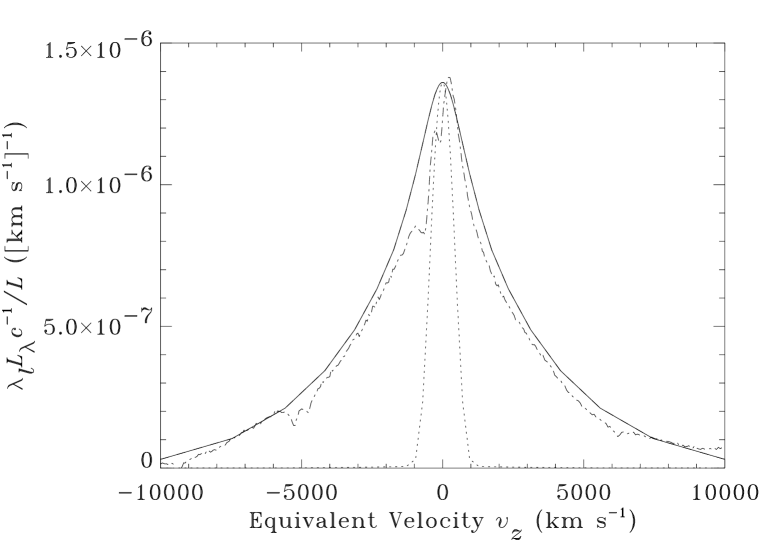
Figure 4.8: Solid line: the C IV $\lambda$1548.20/1550.77 shape of model 2. Dotted line: same line of model 1, scaled to have the same peak flux. Dot-dashed line: NGC 5548, also scaled. Model 1 has a profile that is much narrower than observed. Model 2 lacks the blueshifted absorption feature and apparent redshifted profile base, but fits the NGC 5548 profile well in other respects.

Figure 4.8. The key difference in these profile shapes stems from the higher BLR ($r\leq 50$ light-days) covering that model 2 has due to its enhanced wind area size. The effect this has upon the covering function is shown in Figure 4.3.

Despite the good agreement in the strong lines, there is, nevertheless, poor agreement between the spectrum of NGC 5548 and that of model 2 in several UV lines. For instance, the N IV $\lambda$1486 continuum-subtracted line peak is a factor of 3.7 times stronger in model 2 than in NGC 5548. Similarly, the O III] $\lambda$1664 line flux is a factor of 2.5 times stronger than that of NGC 5548. In addition, like many other published AGN models, the Ly$\alpha$/H$\beta$ ratio of model 2 is 20.8, which is higher than the observed value of 12.6$\pm 2.0$ (e.g., Dumont, Collin-Souffrin, & Nazarova 1998). This problem persists despite the high densities and columns we employ. As discussed in more detail below, several of these types of discrepancies can be removed by invoking different model parameters. However, some discrepancies persist even with many changes. These discrepancies, which we point out throughout this chapter and summarize in Chapter 5, are important problems with the stellar wind model.

The linearized response function for model 2 of the Ly$\alpha$ line flux due to variations of the observed UV ionizing continuum is shown in

Figure 4.9: Solid line: the linearized response function of the Ly$\alpha$ line profile due to variations in the UV continuum luminosity for model 2. Dotted line: the response function of the “summed line” (the synthetic line for which $\epsilon_{l}=1.0$ everywhere) for model 2 scaled down by a factor of 10² in order to fit plot. Dashed line: the summed line response function for model 1 scaled up by a factor of 10 in order to be visible in plot.

Figure 4.9. For comparison, the response function for model 1 is also shown. For model 1, the response function of Ly$\alpha$ is approximately zero at the intermediate delays of $\sim$10-15 days because the cloud area gains are zero (with the area being inversely proportional to the flux) at intermediate distances in the BLR. Conversely, the cloud sizes are independent of the local continuum flux at both low and high radii, giving the cloud areas of model 1 much larger gains (approaching unity) at high delays. Model 2, with $\alpha>0$, is relatively immune from these types of nonlinear effects, which incidentally were not taken into account by AN97.

The response functions of model 2 peak at $\sim$3.3 days. In comparison, Krolik & Done (1995) obtained a peak of approximately $7\pm 4$ days for C IV in NGC 5548. The uncertainty is primarily due to two things. First, there is an ambiguity in the ideal deconvolution algorithm parameters. Second, the sampling rate, which was 4 days, is poor. For these reasons, the peak could be considered as an upper limit to the true peak that would be obtained from a hypothetical infinitely high sampling rate. Incidentally, this also may be the reason that the peak of the NGC 5548 C IV response function obtained from using the 1989 IUE data set with a sampling interval of 4 days, is approximately $7\pm 4$ days (Krolik & Done 1995), while the 1993 data set, with a sampling rate of 1 day, peaks at approximately $0\pm 2$ days (Wanders et al. 1995; Done & Krolik 1996).

Determining where the response function peaks reside is especially important to wind models. This is because the innermost BLR emission radius is the well-defined tidal radius of the stars (eq. [1.6]). The tidal radius $r_{\rm t}$ regulates the size of the geometrical response function. This function can have structure only on time scales greater than $\sim 2r_{\rm t}/c$, or, for model 2, 3.3 days. In most other AGN cloud models, this innermost emission region is a free parameter. Therefore, one way to test wind models is to measure the shortest delay at which the response function has structure, or, as discussed in Appendix I, to measure the highest frequency at which the derivative of the transfer function is nonzero.

The particular nature that this structure takes depends highly upon the anisotropy factor of the line $\epsilon_{{\rm A}l}$. As previously mentioned, the column densities for model 2 are quite high compared to other BLR models (see

Figure 4.10: Solid line, left axis: the mean column density for model 2. Dotted line, right axis: the ionization parameter $\Xi$.

Figure 4.10). This makes the clouds optically thick to Ly$\alpha$. Therefore, the winds at small delays for a given radius (which are at small angles relative to the line of sight) do not emit line radiation towards the observer, but rather mostly emit back towards the continuum source. As a result, the Ly$\alpha$ response function is approximately the shape of a rising triangle for $0\leq\tau\leq 2r_{\rm t}/c$. This is shown in Figure 4.9. A more realistic model accounting for a range of stellar radii and mass, each with a different tidal radius, would have a much smoother response function. The effect of varying the tidal radius is discussed in § 4.13.

An additional characteristic of the Ly$\alpha$ response function (as well as other functions that tend to peak near zero) is its “FWHM,” or full width at half the maximum amplitude. The FWHM of the Ly$\alpha$ response function for model 2 is 13 days. The FWHM obtained by Krolik & Done (1995) was 28 days. Thus, both the peak and the FWHM of the Ly$\alpha$ response function are suggestive of the innermost BLR radius for model 2 being about a factor of 2 smaller than that appropriate for NGC 5548.

However, as will be discussed in more detail in § 4.13, artificially increasing the tidal radius of model 2 would not necessarily improve the overall agreement with the observed response functions of NGC 5548. This is because increasing $r_{\rm t}$ would worsen the fits to the C IV response functions obtained using the 1993 data set. The C IV response function of model 2 is shown in

Figure 4.11: Solid line: the linearized response function for the C IV line of model 2. Dotted line: model 1, increased in scale by factor of 5000.

Figure 4.11. It peaks at 3.3 days. This is larger than the peak at $0\pm\sim 2$ days implied by the results of Done & Krolik (1996) and Wanders et al. (1995). Placing the clouds farther away in model 2 would worsen this discrepancy.

The 1993 data set, in addition to being better sampled on the “blue” end of the power spectrum, also has a higher signal to noise ratio than the 1989 IUE data set—its energy resolution is a mere $\pm 0.25$ Å. This better resolution permitted the first measurements of “velocity-resolved AGN response functions,” or, more correctly, velocity-integrated response functions of profile components.

Figure 4.12: The velocity-integrated linearized response functions of the C IV line profile components due to variations in the continuum luminosity for model 2. Dotted line: wing component. Solid line: the response function for the C IV core component. The peak of the wing response function is a factor of 1.8 higher than the peak of the core response function.

Figure 4.12 shows the velocity-integrated response functions of the “wing” and “core” C IV line profile components for model 2. The velocity cutoff points between the wing and core components were, respectively, $2450$ km s${}^{-1}<|v_{z}|\leq 10,000$ km s^-1 and $0$ km s${}^{-1}\leq|v_{z}|\leq 2450$ km s^-1. These are identical to those assumed by Wanders et al. (1995) and are very close to those employed by Done & Krolik (1995). Due to their simple rising triangle shapes, the wing and core of the model 2 response functions peak at 3.3 days$\approx 2r_{\rm t}/c$. The FWHM is 6 days for the wing component and 11 days for the core component. In comparison, the C IV NGC 5548 response functions published by Wanders et al. (1995) have a FWHM of 16 days for the red and blue cores, 10 days for the red wing, and 24 days for the blue wing. These FWHMs are roughly 50% larger than those of model 2. However, these results employed the SOLA deconvolution algorithm described by Pijpers & Wanders (1994), which extracts response functions rather than linearized response functions, with the difference being that the former uses absolute variations (which incidentally are positive-definite) as input while the latter uses variations about means (which can be negative). Direct comparison with the results shown in 4.12 is thus difficult.

Done & Krolik (1996) also obtained response functions of profile components, but used the regularized inversion deconvolution algorithm (Krolik & Done 1995). They obtained a FWHM of 8 days for the response function of the red core, a FWHM of $\sim$9 days for the blue core, a FWHM of $\sim$6 days for the red wing, and a FWHM of $\sim$11 days for the blue wing. Model 2 agrees much better with these results than the falling, nearly triangular SOLA ones. They do resemble, however, the smoothed response function for the total C IV emission obtained by Done & Krolik (1996) (their Figure 3). Nevertheless, two important problems remain:

1. Model 2 has a perfect red-blue symmetry. Model 2 is, therefore, not fully compatible with NGC 5548 data. This is, in fact, a problem with each of the wind models discussed in this section. Incidentally, it not a problem with the models discussed in Appendix L.

2. The maximum amplitudes of the response functions $\Psi_{F_{l}|F_{\rm c}}(0)$ obtained by Wanders et al. (1995) and Done & Krolik (1996) are roughly the same for each C IV profile component. For model 2, however, the maximum amplitude of the wing component is 1.6 times that of the core component. This discrepancy could be removed by decreasing the velocity dispersion at the tidal radius. As shown in §§ 4.13 & 4.14, this decrease in velocity dispersion can be achieved by decreasing $M_{\rm h}/r_{\rm t}$, but only at the expense of making the C IV profile narrower than observed. Ultimately, this problem arises because the velocity cut points which define the wing and core components are fixed at $\pm$2540 km s^-1, despite the fact that the profile falls off rapidly at equivalent tangential velocities beyond $v_{z}\sim\sigma_{v}$, where $\sigma_{v}=[GM_{\rm h}/(3r_{\rm t})]^{1/2}$ is the velocity dispersion of $f$ at $r=r_{\rm t}$. A velocity dispersion of $\sigma_{v}\mathrel{\hbox{\hbox to0.0pt{\hbox{\lower 5.0pt\hbox{$\sim$}}\hss}\hbox{$>$}}}5000$ km s^-1 is required at $r=r_{\rm t}$ in order to obtain the semi-logarithmic profile out to 10,000 km s^-1 as is observed. So by decreasing $M_{\rm h}/r_{\rm t}$, the wing/core ratio could be reduced, but the width would be increased.

4.3 Models 3 and 4: Varying the Edge Ionization to Pressure Ratio $\Xi/P$

Models 3 and 4 illustrate the effects of varying the ratio of the ionization parameter at the wind edge $\Xi$ to the pressure $P$. Before we discuss these models, let us state why the $\Xi$ parameter alone is not varied and, more generally, how we probe the stellar wind AGN model parameter space.

The parameters of AGN cloud models (including the red giant wind model) can be grouped into two categories depending on which line emission characteristics they affect most:

1. A category that consists of parameters which primarily affects the line ratios. In most AGN models the line ratios are regulated by the emissivities, which are in turn three-dimensional functions of $\Xi$ (or $U$), $P$ (or $n_{\rm H}$), and $N_{\rm c}$, where $L/r^{2}\propto\Xi$ and $P\propto(L/r^{2})^{s/2}$. As mentioned before, because of the very high column densities that we assume, $N_{\rm c}$ is a relatively unimportant parameter for most of the range of parameter space of interest. Also, $L$ is readily observable but time dependent. Thus, for a given observed value of $L$, the $\Xi$ ratio could be adjusted, but not $\Xi$ or $P$ by itself. Conversely, as $L$ changes in an AGN with known a $\Xi$ ratio, both $P$ and $\Xi$ can vary, depending upon the value of $s$ assumed. This section as well as the next two sections explore the line ratio parameter space by varying, respectively, the $\Xi$ ratio (with $L$ fixed) (§ 4.3), $L$ (with $\Xi$ fixed but with changes in $\dot{M}$ to counteract changes to the covering function that would occur otherwise) (§ 4.4), and $s$ (§ 4.5). Thus, we probe the structure of the emissivity function in a non-orthogonal fashion (similar to that of Taylor [1994]). Because the underlying parameters are common to most AGN line emission models, §§ 4.3-4.5 should be of interest to the AGN community whether or not the AGN stellar wind model is actually valid.

2. A category of parameters that does not directly regulate line ratios but rather primarily affects properties specific to the stellar wind AGN line emission model. Parameters in this category primarily affect the covering function, or strength and shape of the “generic line profile.” As mentioned previously (see Fig. 4.9), this generic or “summed” line emission flux is defined to be the synthetic line resulting from a hypothetical line efficiency of unity. (The summed line flux is equal to the incident continuum heating were the clouds completely opaque.) The flux of the summed line is approximately the difference between the spectrum and the continuum. The parameters in this second category can be further subdivided into those which affect the stellar winds and those which affect the stellar distribution function. In the former (winds) subcategory are luminosity $L$ (without compensatory changes in $\dot{M}$) (§ 4.6), the mass loss slope $\alpha$ (§ 4.7), the terminal stellar wind speed $v_{\infty}$ (§ 4.8), the ratio of the stellar mass loss to the terminal wind velocity $\dot{M}/v_{\infty}$ (§ 4.9), the minimum column density $N_{\rm{cmin}}$ (§ 4.10), and the minimum mass loss rate $\dot{M}_{\rm{min}}$ (§ 4.11). In the latter (distribution function) subcategory are the density slope $3-\eta$ (§ 4.12), the tidal radius $r_{\rm t}$ (§ 4.13), the black hole mass $M_{\rm h}$ (§ 4.14), and the cluster mass $M_{\rm c}$ (§ 4.15). In §§ 4.6-4.15 we discuss models which illustrate how each of these parameters affect observable quantities.

Before continuing, note that this partitioning of the model parameters into a line ratio category and a summed line profile category is incomplete even with some of the compensatory changes we make. This is because many parameters affect both. For instance, the tidal radius $r_{\rm t}$ is classified as being a summed line profile parameter. However, by lowering it, one increases the O VI/C IV line ratio for $s<2$ models. This is because the local O VI/C IV ratio is a decreasing function of the distance from the continuum source. Similarly, if the ionization parameter (deemed a ratio parameter) is increased enough, cooling via line emission decreases, which of course would decrease the strength of the summed line.

Models 3 and 4 are similar to model 2 yet have different $\Xi$ ratios. As mentioned earlier, model 2 was given an ionization parameter of $\Xi=1.0$ so that it would be more compatible with observations. This is a full decade lower than that of model 1. Models 3 and 4 have, respectively, an ionization parameter of 0.25 and 4.0 in the BLR. This is shown in

Figure 4.13: Thin lines, left axis: column density $N_{\rm c}$. Thick lines, right axis: wind edge ionization parameter $\Xi$. Dotted lines: model 3. Dashed lines: model 4. Solid lines: model 2, shown for comparison.

Figure 4.13. Note that beyond $1800$ light days, $N_{\rm{c}}=N_{\rm{cmin}}$. In this region, the mass loss is constant, and the edge pressure is nearly constant, so the cloud edge ionization parameter falls as $\sim r^{-2}$.

One effect of increasing $\Xi$ is that it decreases the density at the wind edge. For a given mass loss rate, this increases the radius of the cool portion of the wind, which affects the summed line flux. Unfortunately, several other parameters also affect the summed line flux. Therefore, in order to help isolate just the effect of varying the ionization state of the line-emitting gas without changing the covering factor at the same time, the mass loss rates were also changed in models 3 and 4. Because the mass loss rate affects the wind size (for a given column-density-limited wind), the minimum permissible column density was additionally changed. These modified mass loss rates and column densities for models 3 and 4 are shown, respectively, in Figures 4.14

Figure 4.14: Dotted line: the mass loss rate per star $\dot{M}$ as a function of radius from the black hole $r$ for model 3. Dashed line: model 4. Solid line: model 2.

and 4.13. The resulting effective wind areas for the supergiants of models 3 and 4 are shown in

Figure 4.15: Solid thin line, left axis: the cloud area $A$ as a function of radius $r$ for models 2, 3, and 4. (Due to the adjustments with the mass loss rate and the column density, the area functions are identical for each model.) Thick dotted line, right axis: the radial dependence of the pressure $P_{\rm edge}$ at the wind edge for model 3. Thick dashed line: $P_{\rm edge}$ for model 4. Thick solid line: $P_{\rm edge}$ for model 2.

Figure 4.15.

Spectra of models 3 and 4 are shown in Figures 4.16 and 4.17.

Figure 4.16: Dotted line: hard UV spectrum of model 3. Dashed line: model 4. Solid line: model 2. Dot-dashed line: NGC 5548.

Figure 4.17: Dotted line: soft UV spectrum of model 3. Dashed line: model 4. Solid line: model 2. Dot-dashed line: NGC 5548.

As expected, model 3 ($\Xi=0.25$) has relatively low O VI and N V line fluxes. On the other hand, these lines are relatively bright in model 4 ($\Xi=4.0$). Model 2, with its intermediate yet still high ionization parameter of $\Xi=1.0$, is closest to matching the actual N V line flux that was observed from NGC 5548 by HST.

As

Figure 4.18: Dotted line: C III] spectral region of model 3 ($\Xi=0.25$). Dashed line: model 4 ($\Xi=4.0$). Solid line: model 2 ($\Xi=1.0$). Dot-dashed line: NGC 5548.

Figure 4.18 shows, the C III] $\lambda$1909 Å profile shape is different for each of the three models. This is, however, not true of its integrated intensity, which illustrates a shortcoming of analysis based upon ratios alone. Model 4 ($\Xi=4.0$) has the broadest and weakest C III] profile. Its ionization parameter is very high everywhere, so the C III] flux is necessarily low everywhere. However, because $s=1.9$ in each of these models and the C III] inter-combination line is suppressed at high densities due to quenching, the broader profile components are relatively weak. Model 4 has the lowest density. It is therefore the most immune to this effect. As a result, the high-velocity-dispersion clouds of model 4 have a relatively large C III] flux, which is why this model has the broadest C III] profile. Model 3, on the other hand, has a much lower ionization parameter that nearly maximizes the mean fractional abundance of C⁺² in the line-emitting regions of its clouds, so it is relatively strong in C III] on the whole. Model 3 also has the highest density, so it has the narrowest of the three profiles. Model 2 comes closest to matching the actual C III] profile that is observed in NGC 5548.

Simultaneous comparison of other lines reveals important shortcomings that are intrinsic to these red giant wind models. For instance, the NGC 5548 N IV $\lambda$1486 and the O III] $\lambda$1664 line fluxes are lower than all of the models shown. Model 3 ($\Xi=0.25$) comes closest to matching the observed strength of these lines. However, model 3 fares worst at matching the observed N V line strength. Therefore, provided the other parameters remain constant, no single value of $\Xi$ can simultaneously match each of these line strengths.

In some cases, adjusting additional parameters can help line ratio problems similar to this one. For instance, increasing the metallicity would help increase the nitrogen line fluxes, which are relatively too low in model 3. However, as is discussed in §§ 4.2, 4.4, & 4.6, even permitting each parameter to be freely adjustable would not yield complete agreement with each NGC 5548 line flux.

4.4 Models 4.4 and 4.8: Varying the Luminosity $L$, Pressure $P$, and Mass Loss $\dot{M}$

In the previous subsection, we presented models in which the wind edge pressure and ionization parameter were varied while the luminosity was held constant. In this section, we present models in which the continuum luminosity and cloud pressures were changed, but the ionization parameter was held fixed.

Model 4.4 is similar to model 2 except that its bolometric luminosity is $10^{43}$ ergs s^-1 instead of $3.2\times 10^{43}$ erg s^-1. Model 4.8 has a bolometric luminosity of $10^{44}$ ergs s^-1. The luminosity parameter $L$ is similar to the $\Xi/P$ ratio discussed in the previous subsection in that changing it also affects the covering function. In order to help isolate just the effect of changing $L$ and $P$ upon the line ratios, we again adjusted $\dot{M}$, $\dot{M}_{\rm min}$, and $N_{\rm cmin}$ in models 4.4 and 4.8. This forced the area functions (shown in

Figure 4.19: Solid line, left axis: wind area functions for models 4.4, 4.8, and 2. Thick lines, right axis: wind edge pressures. Dotted line: model 4.4. Dashed line: model 4.8. Solid lines: model 2.

Figure 4.19) and geometrical covering functions to be identical. The full effects of varying the luminosity without any such adjustments are discussed in § 4.6. However, for model 2, $s$ is near $2$, while $\alpha$ is near unity. Therefore, neither the cloud edge ionization parameters nor the cloud area functions are a strong function of the local continuum flux, and the models discussed here are very similar to those of § 4.6.

The UV spectra of models 4.4 and 4.8 are shown in Figures 4.20 and 4.21.

Figure 4.20: Dotted line: model 4.4 ($L=10^{43}$ ergs s^-1). Dashed line: model 6 ($L=10^{44}$ ergs s^-1). Solid line: model 2 ($L=3.2\times 10^{43}$ ergs s^-1). Dot-dashed line: NGC 5548.

Figure 4.21: Dotted line: model 4.4 ($L=10^{43}$ ergs s^-1). Dashed line: model 6 ($L=10^{44}$ ergs s^-1). Solid line: model 2 ($L=3.2\times 10^{43}$ ergs s^-1). Dot-dashed line: NGC 5548.

Because the geometrical covering functions of the models are identical, the equivalent widths of the lines are approximately the same in models 4.4 and 4.8. This is despite the factor of 10 variation in luminosity.

Changing the luminosity does not have a discernible effect upon the absolute C III $\lambda$977 Å line strength. This result is opposite that of Rees, Netzer, & Ferland (1989). The C III $\lambda$977 Å emission characteristics obtained by Rees, Netzer, & Ferland (1989) occurred because of thermalization of strong lines that have high optical depths. This redistributes the cooling to other lines including C III $\lambda$977. Our results do not show such an increase in C III $\lambda$977 except at high densities approaching $10^{12}$ cm^-3, which is outside the parameter space that XSTAR version 1.20 was designed to compute. Such high density models are shown in § 4.6.

On the other hand, the densities and local continuum fluxes of model 4.8 are high enough to suppress the highest velocity components of the Ly$\alpha$ profile (shown at higher resolution in

Figure 4.22: Dotted line: Ly$\alpha$ line of model 4.4. Dashed line: Ly$\alpha$ line of model 4.8. Solid line: Ly$\alpha$ line of model 2. Dot-dashed line: continuum subtracted NGC 5548 time-averaged Ly$\alpha$ spectral region, normalized to match the model 2 profile peak.

Figure 4.22) and the C IV profile (shown in

Figure 4.23: Dotted line: C IV line of model 4.4. Dashed line: C IV line of model 4.8.

Figure 4.23). These lines behave in a fashion similar to C III]—the line efficiencies in the high density models of the clouds nearest to the black hole are suppressed. This results in these models having narrower profiles.

The behavior of the C III] profile itself is shown in

Figure 4.24: Dotted line: C III] profile of model 4.4 ($L=10^{43}$ ergs s^-1). Dashed line: model 4.8 ($L=10^{44}$ ergs s^-1). Solid line: model 2 ($L=3.2\times 10^{43}$ ergs s^-1). Dot-dashed line: NGC 5548.

Figure 4.24. The dependence of the C III] profile shape upon luminosity is perhaps the most prominent difference between models 4.4 and 4.8. This dependence arises for the reasons mentioned in the previous subsection—the higher luminosity model has higher densities, which yield less C III] emission. As a result, the higher luminosity models have narrower profiles.

Note that the broad and narrow components of the observed C III] line blend appear to be shifted towards the blue. In contrast, the line shifts of the synthetic spectra are zero (cf Appendix L). Also, model 4.8 (and to a lesser extent the two other models) does not produce sufficient broad C III] line emission. The time-averaged ionizing luminosity of NGC 5548 and model 4.8 are approximately the same: $\sim 4\times 10^{43}$ ergs s^-1. (For the continuum assumed, the bolometric luminosity of each model is 2.61 times greater than 1-1000 Ry ionizing luminosity). Model 2, which has a luminosity that is a factor of $\sim$3 less than NGC 5548, fairs better in this respect. However, the C III]/C IV line ratio of the broad profile components is too low in all of our models in which the luminosity was the same as the NGC 5548 value. This broad component C III]/C IV line ratio problem was first discussed by Krolik et al. (1991). The problem arises because the continuum flux in the BLR is so high for the Hubble constant of $H=65$ km s^-1 Mpc^-1 that we assumed. That is, because $P=F/(c\Xi\cos\theta)$, a decrease in the ionization parameter results in an increase in the pressure, which increases collisional de-excitation of C III]. Conversely, if the pressure is decreased, the ionizational abundance of C⁺² becomes too low. In this respect, the stellar wind model has two advantages over some of the other models that have been examined. First, the angled region of the optically thick wind effectively has a lower continuum flux at the cloud edge. This permits it to have lower densities and ionization parameters than the face-on cloud models that are traditionally assumed by photoionization codes. Second, the optically thick winds effectively have more than one single ionization parameter. This smoothes the radial dependence of the total C III] emissivity function. Despite these features, our models still exhibit the C III] deficiency. Incidentally, this problem does not exist for the integrated C III]/C IV line ratio, which is an agreeable 6.8^-1 in NGC 5548 (Krolik et al. 1991), 5.4^-1 in model 2, and 5.2^-1 in model 4.8.

Dumont et al. (1998) state that the C III]/C IV problem can be resolved simply by realizing that the response function of the C III] line is more extended (suggesting emission from larger distances) than that of the other lines. Caution should be exercised here, however, for two reasons. First, the C III] line, though narrower than most of the other UV lines, is still a broad line. Moving the emission covering function out would only reduce the broad emission flux even further. (At issue should be only the flux of the broader C III] components.) Second, the gain of the broad component of the C III] line is much less than that of other UV lines (compare Figures 4.25

Figure 4.25: Dotted line: the model-independent asymptotic gain of the C III] line with respect to variations in the pressure as a function of $2r/c$ for model 4.4 ($L=10^{43}$ ergs s^-1). Dashed line: model 4.8 ($L=10^{44}$ ergs s^-1). Solid line: model 2 ($L=3.2\times 10^{43}$ ergs s^-1).

and 4.26

Figure 4.26: As in Figure 4.25, but for the Ly$\alpha$ line.

). For this reason, its response function is more extended than its “spatial response function” that would exist if the line responded linearly. Thus the large FWHM of the linearized response function of this line does not necessarily translate to an extended emission region.

On the other hand, our models assume a much harder continuum than the one shown in Dumont et al. (1998); our models may have a time-averaged ionizing continuum luminosity that is too high. The issue is complicated by time variability. Fully nonlinear time evolution models which fully account for such effects may someday help resolve whether or not the C III]/C IV ratio problem is significant.

4.5 Models 5 and 6: Varying the Pressure Slope $s$

This subsection discusses models that have different values of the pressure slope parameter $s$ (where $P\propto[L/r^{2}]^{s/2}$ and $\Xi\propto[L/r^{2}]^{1-s/2}$). In model 5, $s=1.0$, $\alpha=0.65$, $\dot{M}_{\rm min}=1.7\times 10^{-5}\,M_{\odot}$ yr^-1, and $N_{\rm cmin}=1.4\times 10^{23}$ cm^-2. In model 6, $s=1.5$, $\alpha=0.90$, $\dot{M}_{\rm min}=8.7\times 10^{-7}\,M_{\odot}$ yr^-1, and $N_{\rm cmin}=7.2\times 10^{21}$ cm^-2. As

Figure 4.27: Thin lines, left axis: column density $N_{\rm c}$. Thick lines, right axis: wind edge ionization parameter $\Xi$. Dotted lines: model 5 ($s=1.0$). Dashed lines: model 6 ($s=1.5$). Solid lines: model 2.

Figure 4.27 shows, the pressure slope $s$ gives the dependence of the ionization parameter upon position within the BLR. Thus, $s$ affects the line emissivities and ratios. It also affects the summed line by changing the area function. This changing of the covering function is not of interest here because it is discussed in §§ 4.6-4.15. By adjusting $\alpha$, $\dot{M}_{\rm min}$, and $N_{\rm cmin}$ in addition to $s$, we help isolate the effect that changing $s$ has upon just the line ratios and emissivities. This also keeps the approximation of the asymptotic area gain given by equation (3.5) to be constant at +0.15. The wind area functions of models 4 and 5 are shown in

Figure 4.28: Thin lines, left axis: wind area functions. Thick lines, right axis: wind edge pressures. Dotted lines: model 5. Dashed lines: model 6. Solid lines: model 2.

Figure 4.28. Note that these adjustments are not totally complete; in the relatively unimportant outer portion of the NLR the models have slightly different area functions.

Spectra of models 5 and 6 are shown in Figures 4.29 and 4.30.

Figure 4.29: Dotted line: model 5 ($s=1.0$). Dashed line: model 6 ($s=1.5$). Solid line: model 2 ($s=1.9$).

Figure 4.30: Dotted line: model 5 ($s=1.0$). Dashed line: model 6 ($s=1.5$). Solid line: model 2 ($s=1.9$).

The intermediate-ionization lines of the spectrum of model 5 ($s=1.0$) are broader than the low-ionization and recombination lines. This is especially apparent for the C IV, C III], and O VI profiles, which are much broader than those of model 2.

Figure 4.31: Dotted lines: model 5 ($s=1.9$) line profiles. Solid lines: model 2 ($s=1.0$) line profiles. Thick lines: Ly$\alpha$. Thin lines: C IV. The $y$-axis scale is applicable only for the C IV $\lambda$1548.2 Å line flux of model 2; the other lines were rescaled. This plot confirms that the $s$ parameter affects C IV much more than Ly$\alpha$.

Figure 4.31 shows this effect more clearly. This broadening occurs if $s<2.0$ because the ionization of low-velocity-dispersion clouds becomes too low for substantial line emission to occur. Since Ly$\alpha$ is a recombination line, it is relatively immune to this effect. These results imply $s\mathrel{\hbox{\hbox to0.0pt{\hbox{\lower 5.0pt\hbox{$\sim$}}\hss}\hbox{$>$}}}1.7$. Comparable results were obtained by Rees et al. (1989). On the other hand, several of the model 5 ($s=1.0$) line shapes and fluxes are in closer agreement with NGC 5548 than model 2. This is particularly evident for the N IV $\lambda$ 1486 and O III] $\lambda$1664 lines. Thus, no value of $s$ would simultaneously fit all features of the NGC 5548 spectrum. This poses yet another (admittedly minor) problem for these wind AGN models.

The response functions of models 5 and 6 also illustrate the effects of varying the ionization gradient in the BLR. The response functions of C IV for models 5 and 6 are shown in

Figure 4.32: C IV response functions. Dotted line: model 5 ($s=1.0$). Dashed line: model 6 ($s=1.5$). Solid line: model 2 ($s=1.9$).

Figure 4.32. In accordance with $\Xi\propto[L/r^{2}]^{1-s/2}$, the response drops off much more rapidly in the $s=1.0$ model than it does in the $s=1.9$ model.

Many of the differences between the three response functions shown are caused by differences in the gains. The radial dependences of the C IV line flux gains are in

Figure 4.33: The gains of the C IV line emission from stellar winds due to variations of the continuum luminosity as a function of radius $r$. Dotted line: model 5 ($s=1.0$). Dashed line: model 6 ($s=1.5$). Solid line: model 2 ($s=1.9$).

Figure 4.33. The two key functions that regulate these gains are $\eta(\epsilon_{l}|\Xi)$ and $\eta(\epsilon_{l}|P)$, shown, respectively, in Figures 4.34 and 4.35.

Figure 4.34: The asymptotic gain of the C IV line emissivity due to variations of the ionization parameter. Dotted line: model 5 ($s=1.0$). Dashed line: model 6 ($s=1.5$). Solid line: model 2 ($s=1.9$).

Figure 4.35: The asymptotic gain of the C IV line emissivity due to variations of the wind edge pressure. Dotted line: model 5 ($s=1.0$). Dashed line: model 6 ($s=1.5$). Solid line: model 2 ($s=1.9$).

Only the $s=1.0$ model has low enough ionization for $\eta(\epsilon_{l}|\Xi)\gg 1$ to occur within 100 light-days from the black hole.

The Ly$\alpha$ response functions of models 5 and 6 are shown in

Figure 4.36: Ly$\alpha$ response functions. Dotted line: model 5 ($s=1.0$). Dashed line: model 6 ($s=1.5$). Solid line: model 2 ($s=1.9$). Though difficult to see from this view of the data, the response function of model 5 falls the fastest and has the weakest relative response at intermediate delays.

Figure 4.36. As Figures 4.37, 4.38, and 4.39 show, for these models Ly$\alpha$ is relatively more sensitive to increases in pressure than ionization. This is due to high optical depths and thermalization of Ly$\alpha$ at high pressures (as in Rees et al. 1989). This causes model 2, which has the lowest average pressure (see Fig. 4.28), to have the strongest emissivity at intermediate distances ($2r/c\sim 10$ days). This difference gives rise to the relatively steep drop in the Ly$\alpha$ response function of model 5.

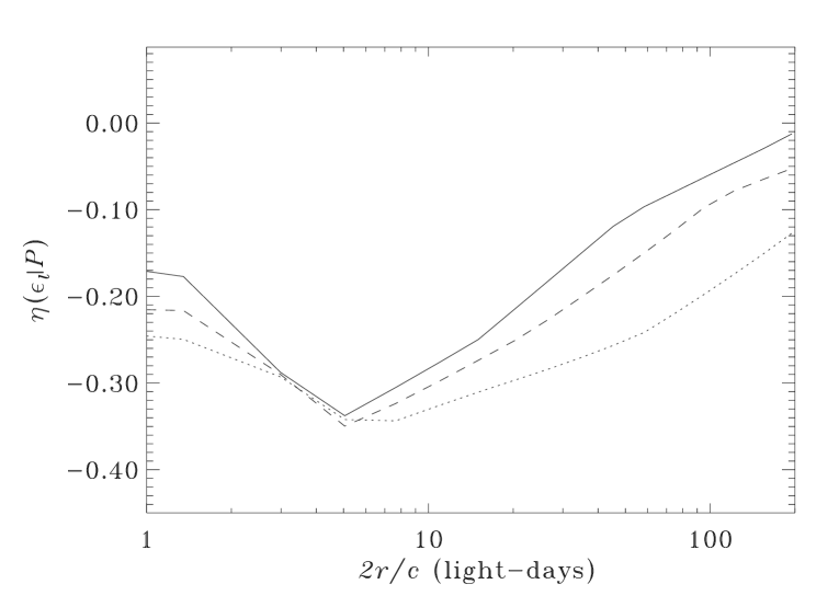
Figure 4.37: The asymptotic gain of the Ly$\alpha$ line emissivity due to variations of the wind edge pressure. Dotted line: model 5 ($s=1.0$). Dashed line: model 6 ($s=1.5$). Solid line: model 2 ($s=1.9$).

Figure 4.38: The asymptotic gain of the Ly$\alpha$ line emissivity due to variations of the wind edge ionization parameter. Dotted line: model 5 ($s=1.0$). Dashed line: model 6 ($s=1.5$). Solid line: model 2 ($s=1.9$).

Figure 4.39: The emissivity of the Ly$\alpha$ line as a function of radius. Dotted line: model 5 ($s=1.0$). Dashed line: model 6 ($s=1.5$). Solid line: model 2 ($s=1.9$). Note that the pressures are so high that this line becomes thermalized near the black hole, especially for model 5.

4.6 Models 7, 8, and 9: Varying the Luminosity $L$

Models 3-6, discussed in the three previous sections, illustrate the effects of changing parameters which affect the line ratios, but not the covering function. In the remaining sections of this chapter, we present models which illustrate the effects of varying not only the line ratios, but also the covering function, which is in turn determined by the wind area and stellar distribution functions. Unlike the results in §§ 4.3-4.5, the results in the remaining sections of this chapter probably have significance only if the stellar wind line emission model is correct.

Model 7 is a variant of model 1. Its bolometric luminosity is $10^{45}$ ergs s^-1 instead of the $10^{44}$ ergs s^-1 of model 1. The wind area function of model 7 is shown in

Figure 4.40: Thin lines, left axis: wind area functions. Thick lines, right axis: wind edge pressures. Dotted lines: model 7. Solid lines: model 1.

Figure 4.40. Note that the effective sizes $r_{\rm BLR}$ of the line emission regions contributing towards the broader profile components of models 1 and 7 are determined primarily by the wind area functions rather than some other parameters of the covering functions, such as the tidal radii. For models similar to models 1 and 7, the most important effect of increasing the luminosity is that $r_{12}$ increases, with $r_{12}\simeq r_{\rm BLR}\propto L^{1/2}$ in particular, where $r_{12}$ again denotes the outermost position where the winds begin to be fully “stripped.”

This prediction of model 1 is based upon the Kazanas (1989) paper. It agrees with the first reverberation mapping campaign results for luminous quasars. Kaspi et al. (1996), who published these results based on reverberation mapping of 12 AGNs, conclude that they are indeed compatible with $r_{\rm BLR}\propto L^{1/2}$. Any model which invokes evaporation of clouds that have internal pressure gradients could yield this important result. However, with the notable exception of stellar wind models, few such potential models could permit their clouds to draw upon the required large reservoirs of replenishing gas. Therefore, the non-stellar models are probably fundamentally incompatible with the evaporative mechanism in the first place (§ 3.1.1).

The line profile of Ly$\alpha$ for model 7 is shown in

Figure 4.41: Dotted line: Half-profile of Ly$\alpha$ for model 7 ($L=10^{45}$ ergs s^-1). Solid line: half-profile of Ly$\alpha$ for model 2 ($L=10^{44}$ ergs s^-1).

Figure 4.41. The FWHM for model 2 is 395 km s^-1, while the FWHM for model 7 is 330 km s^-1. This narrowing is as expected, since the higher fluxes strip/ablate the winds of the high-velocity stars nearest to the black hole. As a result, the covering comes from farther out, and the broad components that would contribute towards the profile are suppressed. Also, the covering factor decreases. Incidentally, if one assumes that the black hole dominates the stellar dynamics, one obtains for a hypothetical linear line the relation $v_{\rm FWHM}\propto L^{-1/4}$ as the time-averaged luminosity $L$ of an individual AGN varies. This yields a much smaller FWHM for model 7 of 222 km s^-1. However, this relation is inapplicable here because the dominant covering function for both of these models is from narrow line clouds residing far enough away that the cluster is likely to dominate the stellar dynamics.

Model 2 violates the theoretical $r_{\rm BLR}\propto L^{1/2}$ relationship much more strongly than model 1. This is because the covering function of model 2 peaks at the tidal radius, regardless of the small variations in the wind area function. This is illustrated by models 8 and 9, which are identical to model 2 with the exception of their bolometric continuum luminosities of $3.16\times 10^{44}$ and $3.16\times 10^{45}$ ergs s^-1 respectively. These luminosities are a factor of 10 and 100 times higher than that of model 2. Unlike the models shown in § 4.4, no other wind parameters were changed. As a result, models 8 and 9 have different area and covering functions. The wind area and pressure functions of models 8 and 9 are shown in

Figure 4.42: Thin lines, left axis: wind area functions. Thick lines, right axis: wind edge pressures. Dotted lines: model 8 ($L=3.16\times 10^{44}$). Dashed lines: model 9 ($L=3.16\times 10^{45}$ ergs s^-1). Solid lines: model 2 ($L=3.16\times 10^{43}$ ergs s^-1).

Figure 4.42. The wind edge pressures of the models scale according to $P\propto(L/r^{2})^{s/2}$, where $s=1.9$. As a result, nearly all of the additional flux is “transferred” to the edge pressure rather than the edge ionization parameter shown in

Figure 4.43: Thin lines, left axis: column density $N_{\rm c}$. Thick lines, right axis: wind edge ionization parameter $\Xi$. Dotted lines: model 8. Dashed lines: model 9. Solid lines: model 2.

Figure 4.43.

The Ly$\alpha$ profiles of models 8 and 9 are shown in

Figure 4.44: Ly$\alpha$ line profiles. Dotted line: model 8 ($L=3.16\times 10^{44}$). Dashed line: model 9 ($L=3.16\times 10^{45}$ ergs s^-1). Solid line: model 2 ($L=3.16\times 10^{43}$ ergs s^-1). Dot-dashed line: NGC 5548. Note that, for the reasons discussed in the text, results for models 9 are not necessarily accurate.

Figure 4.44. The profile strengths and shapes are similar to the ones shown in § 4.4 in that higher pressures result in less Ly$\alpha$ emission. However, the higher luminosity models have slightly enhanced emission in many of the lines such as O VI and N V. This is due to the fact these lines have much smaller optical depths and that $\alpha=1.1>1$ for these models; higher luminosities correspond to a larger summed line flux.

The electron density at the wind edges for clouds in model 9 at the tidal radius is $2.4\times 10^{12}$ cm^-3. This density is near the $10^{12-13}$ cm^-3 limit beyond which XSTAR version 1.20 results may be invalid.

The effect of varying $L$ upon the response function of the artificial summed line is shown in

Figure 4.45: The summed line response function. Dotted line: model 8 ($L=3.16\times 10^{44}$). Dashed line: model 9 ($L=3.16\times 10^{45}$ ergs s^-1). Solid line: model 2 ($L=3.16\times 10^{43}$ ergs s^-1).

Figure 4.45. Because $r_{12}\simeq r_{\rm t}\simeq r_{\rm BLR}$, the luminosity alone has little effect upon $r_{\rm BLR}$. However, since $\dot{M}_{\rm h}$ is likely to be a function of $M_{\rm h}$ (among other parameters), these models do not necessarily indicate the measurable variation of the response functions as a function of $L$ for models similar to model 2. Rather, they merely indicate the intrinsic asymptotic changes for one particular AGN similar to model 2 as its luminosity changes with time. They indicate, for example, the linearized response functions that would be obtained from an AGN that switches from a high state to a low state in a time that is much longer than $r_{\rm BLR}/c$. (Incidentally, such a change from a high to low state could itself permit measurement of the response functions on time scales much longer than $r_{\rm BLR}/c$.) The most important feature of these response functions is that they all peak at $2r_{\rm t}/c$ regardless of the luminosity. This implies, for profiles of hypothetical lines that respond linearly, $v_{\rm FWHM}\propto L^{0}$ in AGNs with a fixed black hole mass.

The (nonlinear) effects of varying $L$ upon the Ly$\alpha$ response functions are shown in

Figure 4.46: Response functions of Ly$\alpha$. Dotted line: model 8 ($L=3.16\times 10^{44}$). Dashed line: model 9 ($L=3.16\times 10^{45}$ ergs s^-1). Solid line: model 2 ($L=3.16\times 10^{43}$ ergs s^-1). For the reasons discussed in the text, results for models 9 are not necessarily accurate.

Figure 4.46. Thermalization makes the line efficiency go down at higher luminosities. This makes many of the strong lines, especially Ly$\alpha$, get weaker even though the summed line gets stronger.

Another way of viewing the above results is through the behavior of $-(2\alpha-s+3-\eta)$, the covering slope in the “optically thick” region. If this slope is steep (negative) enough (e.g., $\alpha\simeq 1$ and $3-\eta\simeq 2$), $r_{\rm BLR}$ is simply a function of the radius of the innermost BLR emission of radius, which is $r_{\rm t}$ for these models. On the other hand, if the slope is shallow (not as negative) enough, the outermost emission radius becomes more important than the innermost emission radius and parameters such as $N_{\rm c}$ and $r_{\rm c}$ would become important. Finally, if the slope changes sharply with radius but is initially shallow because, e.g., $\alpha\simeq 0$ (as in model 1), then the BLR response depends upon the wind parameters of which $r_{12}$ is a function and one can obtain $r_{\rm BLR}\propto L^{1/2}$.

4.7 Models 10 and 11: Varying the Mass Loss Slope $\alpha$

Models 10 and 11 show the effects of varying mass loss slope parameter $\alpha$. In model 10, $\alpha=0.95$. In model 11, $\alpha=1.35$. As equation (4.2) shows, the slope of the radially dependent covering function $An_{*}$ includes a term of $-2\alpha$. This is because $\alpha$ affects the mass loss rates of the wind via $\dot{M}\propto(L/r^{2})^{\alpha}$. For model 2, equation (4.2) yields a covering slope in the optically thick region of $\simeq-1.8$. Increasing $\alpha$ steepens the covering functions, makes the profiles broader and less concave, and increases the gain. Conversely, decreasing $\alpha$ narrows the profiles, makes them more concave, and lowers the gain.

The wind area functions for models 10, 11, and 2 are shown in

Figure 4.47: Thin lines, left axis: wind area functions for models 10, 11, and 2. Thick lines, right axis: cloud edge pressures. Dotted lines: model 10 ($\alpha=0.95$). Dashed lines: model 11 ($\alpha=1.35$). Solid lines: model 2 ($\alpha=1.10$).

Figure 4.47. Scaled profiles of the Ly$\alpha$ line for models 10, 11, and 2 are shown in

Figure 4.48: Scaled Ly$\alpha$ line profiles. Dotted line: model 10 ($\alpha=0.95$), scaled to match the line peak of model 2. Dashed line: model 11 ($\alpha=1.35$), scaled to match the line peak of model 2. Solid line: model 2 ($\alpha=1.10$). Dot-dashed line: NGC 5548, scaled to match line peak of model 2.

Figure 4.48. As expected, the high-$\alpha$ model has the broadest profile. Model 1 (in which $\alpha=0$) is an extreme case illustrating how lowering $\alpha$ narrows the profiles (see Fig. 4.2). Unlike most of the cases discussed above, $\alpha$ has only a small effect upon the BLR line ratios and, more precisely, the intensities as a function of velocity dispersions. Thus, these changes in Ly$\alpha$ are representative of the other lines.

Nevertheless, because of the inherent radial dependences of the line emissivities upon radius, $\alpha$ does indirectly affect several parameters including the line shapes and ratios. This is illustrated by

Figure 4.49: Ly$\alpha$/N V blend. Dotted line: model 10 ($\alpha=0.95$). Dashed line: model 11 ($\alpha=1.35$). Solid line: model 2 ($\alpha=1.10$). Dot-dashed line: NGC 5548. Note the relative narrowness of the N V line of model 10.

Figure 4.49. The profiles of the $\alpha=0.95$ models are so narrow that the N V emission line appears similar in form to systems with blueshifted absorption. No such absorption, however, was accounted for in the model, and the effect is purely due to the narrowness of the $\alpha=0.95$ lines.

Figure 4.49 also shows that raising $\alpha$ lowers the covering factor. This is because the stellar wind mass loss functions of models 2, 10, and 11 are normalized to be the same at $r\simeq r_{\rm t}$ (near the inner edge of the BLR), but model 11 has the steepest radial mass loss gradient. Models 10 ($\alpha=0.95$) and 2 ($\alpha=1.10$) thus have higher NLR coverings even though each of the models have similar very broad line region coverings.

These effects translate to the other observable quantities of the system, such as the response functions. Response functions for the Ly$\alpha$ line of models 10 and 11 are shown in

Figure 4.50: Response functions for Ly$\alpha$. Dotted line: model 10 ($\alpha=0.95$). Dashed line: model 11 ($\alpha=1.35$). Solid line: model 2 ($\alpha=1.10$).

Figure 4.50. Though the response function peak at $\tau=2r_{\rm t}/c$ for model 10 is only 1.4 times higher than that of model 11, it is 12 times higher at $\tau=98$ days. While the former increase is due primarily to the $\alpha$ term in the expression of the gain (eq. [3.5]) for clouds at $r\sim r_{\rm t}$, the latter increase is due to the fact that $\alpha$ strongly affects the ratio of the NLR covering to the BLR covering.

4.8 Model 13: Varying the Terminal Wind Speed $v_{\infty}$ and the Mass Loss $\dot{M}$

The terminal wind speed $v_{\infty}$ is the maximum outward velocity attained by the stellar winds that reprocess the continuum radiation. For models 1 and 2, we assume $v_{\infty}=10$ km s^-1. As equation (3.3) shows, changing $v_{\infty}$ would affect the cloud areas, with $A\propto\dot{M}/v_{\infty}$. Thus, lowering $v_{\infty}$ or increasing $\dot{M}$ would increase the covering factor, provided all other parameters remained the same. This is discussed in more detail in § 4.9. If both $\dot{M}$ and $v_{\infty}$ were changed by the same factor, but $N_{\rm{cmin}}$ were unchanged, there would be only two major observable changes in the model:

1. the cumulative mass lost by all of the stars, and

2. the equivalent width of absorption features due to stellar winds.

In this section, we address the first of these two characteristics. Some aspects of absorption are discussed in Appendix K.

In model 13, both $v_{\infty}$ and the mass loss function $\dot{M}$ were reduced to 6% of the values assumed in model 2. The cumulative mass lost by all stars is shown in

Figure 4.51: Total mass loss due to reprocessing stellar winds inside distance from the black hole $r$. Dotted line: model 13 ($v_{\infty}=0.6$ km s^-1). Solid line: model 2 ($v_{\infty}=10$ km s^-1).

Figure 4.51. If one assumes that all the gas lost by the stars is accreted, lowering $v_{\infty}$ permits traditional accretion disk efficiencies of $\sim$10%.

It is possible, however, that only a small fraction of this mass would be accreted. The hot plasma deposited into the intercloud medium by stellar winds could, for instance, form a slow-moving outbound AGN superwind, accelerated in part from the twisted magnetic fields of the accretion disk below. Alternatively, the hot plasma deposited by winds could have a non-zero average angular momentum vector aligned with the disk. In this case, the accretion disk must remove the angular momentum by expanding before any additional material could be accreted onto the black hole. The point is that the stellar wind mass loss rate is probably not equal to the accretion rate onto the black hole (which is relatively easy to measure).

At any rate, $v_{\infty}$ is easily measurable in giants and supergiants. It could therefore be argued that it is one of the least uncertain parameters in the wind AGN line emission model. Common measurements yield $v_{\infty}\simeq 10$ km s^-1. AN97 assumed $\textrm{max}(v)\sim 0.1$ km s^-1 for some of their models. This maximal velocity is a factor of 100 less than the observed value. It is a factor of $10^{3}$ less than the $100$ km s^-1 gravitational escape velocities typically observed in giants. Note that thermally driven winds with $v_{\infty}\ll(2GM_{*}/R_{*})^{1/2}\sim 100$ km s^-1 should actually accrete onto their stars. Though red giant winds are not suspected as being thermally driven, we believe that very slow winds are probably not plausible.

Incidentally, very slow winds like those considered by AN97 would probably be more susceptible to pressure from the intercloud medium. This is discussed in detail in Appendix E. In this context, it has been proposed that the stars are not producing winds at all, but rather act as “condensation sites” of a super-heated intercloud medium. Such models are not, however, considered in this work.

4.9 Models 16 and 17: Varying the Mass Loss to Terminal Wind Speed ratio $\dot{M}/v_{\infty}$

Models 16 and 17 are identical to model 2 except for their mass loss rates, which are, respectively, 3.0 times lower and 3.0 higher than that of model 2. This is shown in

Figure 4.52: Mass loss rates per reprocessing wind. Dotted line: model 16. Dashed line: model 17. Solid line: model 2.

Figure 4.52. Since the wind areas are proportional to $\dot{M}/v_{\infty}$, the lowest mass loss model (model 16) also has the least BLR covering. This is shown in

Figure 4.53: Radial covering functions of models 16, 17, and 2. Dotted line: model 16. Dashed line: model 17. Solid line: model 2.

Figure 4.53.

Figure 4.54: The spectral regions near the C IV lines. Dotted line: model 16. Dashed line: model 15. Solid line: model 2. Dot-dashed line: NGC 5548.

Figure 4.54 shows the effect that varying $\dot{M}/v_{\infty}$ has upon the line strengths. The response functions scale with $\dot{M}/v_{\infty}$ in the same way.

Since $\dot{M}_{\rm min}$ was not changed in these three models, the position closest to the continuum source where $\dot{M}=\dot{M}_{\rm min}$ first occurs is nearest to the black hole for model 16 and farthest from the black hole in model 17. For this reason, the lowest mass loss model (model 16) has the highest NLR/BLR covering ratio, as Figures 4.53 and 4.55

Figure 4.55: Thin lines, left axis: wind area functions. Thick lines, right axis: wind edge pressures. Dotted lines: model 16. Dashed lines: model 15. Solid lines: model 2.

show. On the other hand, had $\dot{M}_{\rm min}$ also been changed by the same factor that $\dot{M}$ had been changed, the scaled covering functions would have been unaffected. The effect upon the Ly$\alpha$ profile shape of varying $\dot{M}$ is shown in

Figure 4.56: Ly$\alpha$ profile shapes. Dotted line: model 16, scaled to the peak of the model 2 profile. Dashed line: model 17, scaled to the peak of the model 2 profile. Solid line: model 2.

Figure 4.56. As expected, model 16, which has the lowest $\dot{M}$, has the narrowest Ly$\alpha$ profile.

Incidentally, the C IV profile shapes of these three models are nearly identical. This is because the emissivity of C IV is so low in the NLR.

4.10 Models 14 and 15: Varying the Minimum Column Density $N_{\rm cmin}$

As discussed previously, the minimum column densities of our models are denoted by the parameter $N_{\rm{cmin}}$. This parameter serves as a reservoir for storing our ignorance about possible disruption mechanisms that might affect the more tenuous winds located far from the black hole. Models 14 and 15 show the effect of varying $N_{\rm{cmin}}$. They are identical to model 2 except for their $N_{\rm{cmin}}$ parameters, which are $N_{\rm{cmin}}=3\times 10^{21}$ cm^-2 for model 14 and $N_{\rm{cmin}}=3\times 10^{22}$ cm^-2 for model 15.

The area functions of these models are shown in

Figure 4.57: Thin lines, left axis: wind area functions of models 14, 15, and 2. Thick lines, right axis: wind edge pressures. Dotted lines: model 14 ($N_{\rm{cmin}}=3\times 10^{21}$ cm^-2). Dashed lines: model 15 ($N_{\rm{cmin}}=3\times 10^{22}$ cm^-2). Solid lines: model 2 ($N_{\rm{cmin}}=8\times 10^{22}$ cm^-2). Because the edge pressures are fixed at the outermost emission regions computed in the model (where $N_{\rm{c}}=N_{\rm{cmin}}$), the edge pressures in the NLR are lowest for model 14. For the same reason, model 14 has the highest narrow line ionization parameter and NLR continuum optical depths of these three models.

Figure 4.57. Lowering $N_{\rm{cmin}}$ permits the winds to follow their $A\propto r^{2}$ expansion phase out to regions farther away from the black hole. (For the models considered here, $N_{\rm{c}}=N_{\rm{cmin}}$ occurs farther from the continuum source than does $\dot{M}=\dot{M}_{\rm min}$.)

As a result, lowering $N_{\rm{cmin}}$ enhances the NLR covering. This is shown in

Figure 4.58: Integrated covering as a function of radius. Dotted line: model 14 ($N_{\rm{cmin}}=3\times 10^{21}$ cm^-2). Dashed line: model 15 ($N_{\rm{cmin}}=3\times 10^{22}$ cm^-2). Solid line: model 2 ($N_{\rm{cmin}}=8\times 10^{22}$ cm^-2).

Figure 4.58. The effects upon the profiles and other observables are as one would expect. For instance, the Ly$\alpha$ profile for model 14 ($N_{\rm{cmin}}=3\times 10^{21}$ cm^-2), which is shown in

Figure 4.59: Ly$\alpha$ profiles. Dotted line: model 14 ($N_{\rm{cmin}}=3\times 10^{21}$ cm^-2). Dashed line: model 15 ($N_{\rm{cmin}}=3\times 10^{22}$ cm^-2). Solid line: model 2 ($N_{\rm{cmin}}=8\times 10^{22}$ cm^-2).

Figure 4.59, is narrower than that of model 15 ($N_{\rm{cmin}}=3\times 10^{22}$ cm^-2). Because the winds are optically thin near $N_{\rm{c}}=N_{\rm{cmin}}$, our approximation for the summed line profile (see

Figure 4.60: Profiles of the summed line using the assumption that all of the exposing continuum flux is absorbed by the NLR winds, which is not the case. Dotted line: model 14 ($N_{\rm{cmin}}=3\times 10^{21}$ cm^-2). Dashed line: model 15 ($N_{\rm{cmin}}=3\times 10^{22}$ cm^-2). Solid line: model 2 ($N_{\rm{cmin}}=8\times 10^{22}$ cm^-2). Note that the differences between these profiles are much greater than those for the Ly$\alpha$ profiles (shown in Fig. 4.59).

Figure 4.60) is much more strongly affected by $N_{\rm{cmin}}$.

For the volume of parameter space near model 2, the BLR covering is unaffected by $N_{\rm{cmin}}$. Thus, the response functions at lags below $\sim$1000 days are not functions of $N_{\rm{cmin}}$. Lines which have negligible emission in the NLR (e.g., C IV), are also unaffected by $N_{\rm{cmin}}$.

However, this is not be the case for all possible models, especially those very different from model 2. This is not only because $N_{\rm{cmin}}$ affects the covering, but also because it affects the effective ionization of the outermost clouds.

4.11 Models 18 and 19: Varying the Minimum Mass Loss Rate $\dot{M}_{{\rm min}}$

The mass loss functions of models 18 and 19 are shown in

Figure 4.61: Mass loss rates for stellar winds assumed to be reprocessing continuum radiation into line radiation. Dotted line: model 18 ($\dot{M}_{{\rm min}}=2.4\times 10^{-8}\,\dot{M}_{\odot}$ yr^-1). Dashed line: model 19 ($\dot{M}_{{\rm min}}=2.6\times 10^{-7}\,\dot{M}_{\odot}$ yr^-1). Solid line: model 2 ($\dot{M}_{{\rm min}}=7.9\times 10^{-8}\,\dot{M}_{\odot}$ yr^-1).

Figure 4.61.

Figure 4.62: Thin lines, left axis: wind area functions. Thick lines, right axis: wind edge pressures. Dotted lines: model 18 ($\dot{M}_{{\rm min}}=2.4\times 10^{-8}\dot{M}_{\odot}$ yr^-1). Dashed lines: model 19 ($\dot{M}_{{\rm min}}=2.6\times 10^{-7}\,\dot{M}_{\odot}$ yr^-1). Solid lines: model 2 ($\dot{M}_{{\rm min}}=7.9\times 10^{-8}\,\dot{M}_{\odot}$ yr^-1).

Figure 4.62 shows the wind area functions of models 18 and 19, which have, respectively, minimum mass loss rates 3.4 times less than and greater than that of model 2.

The minimum mass loss parameter $\dot{M}_{{\rm min}}$ is the mass loss assumed for the giants far enough away from the AGN environment that they are unaffected by it. The impact-parameter-averaged wind column densities obey $N_{\rm c}\propto\sqrt{\dot{M}P/v_{\infty}}$, so increasing $\dot{M}_{{\rm min}}$ increases the column densities of the NLR clouds. In $\alpha>0$ models such as the ones considered here, $\dot{M}_{{\rm min}}$ thus regulates where the condition $N_{\rm{c}}\geq N_{\rm{cmin}}$ forces $A$ to be constant at its maximum value; increasing $\dot{M}_{{\rm min}}$ increases the (relatively small) region where $A\propto r^{2}$. As

Figure 4.63: Thin lines, left axis: column density $N_{\rm c}$. Thick lines, right axis: wind edge ionization parameter $\Xi$. Dotted lines: model 18 ($\dot{M}_{{\rm min}}=2.4\times 10^{-8}\,\dot{M}_{\odot}$ yr^-1). Dashed lines: model 19 ($\dot{M}_{{\rm min}}=2.6\times 10^{-7}\,\dot{M}_{\odot}$ yr^-1). Solid lines: model 2 ($\dot{M}_{{\rm min}}=7.9\times 10^{-8}\,\dot{M}_{\odot}$ yr^-1).

Figure 4.63 shows, models with high $\dot{M}_{{\rm min}}$ have high NLR mass losses and column densities. They attain $\dot{M}=\dot{M}_{{\rm min}}$ relatively near the continuum source and $A(r)=\textrm{max}(A)$ relatively far from the continuum source. Their NLR geometrical wind areas are, therefore, relatively large.

From a perspective of model fitting, $\dot{M}_{{\rm min}}$ does nearly the opposite of the $N_{\rm{cmin}}$ parameter discussed in § 4.10—increasing $\dot{M}_{{\rm min}}$ or decreasing $N_{\rm{cmin}}$ will increase the NLR to BLR covering ratio, narrow the profiles (see

Figure 4.64: Ly$\alpha$ line profiles. Dotted line: model 18 ($\dot{M}_{{\rm min}}=2.4\times 10^{-8}\,\dot{M}_{\odot}$ yr^-1). Dashed line: model 19 ($\dot{M}_{{\rm min}}=2.6\times 10^{-7}\,\dot{M}_{\odot}$ yr^-1). Solid line: model 2 ($\dot{M}_{{\rm min}}=7.9\times 10^{-8}\,\dot{M}_{\odot}$ yr^-1).

Figure 4.64), and slightly flatten the response functions at extreme delays. However, the optical depths of the NLR clouds are functions of both the $\dot{M}_{{\rm min}}$ and $N_{\rm{cmin}}$ parameters.

Because the results of varying $\dot{M}_{{\rm min}}$ are so nearly reversed to those associated with varying $N_{\rm{cmin}}$, we do not show other observable properties of models 18 and 19 here; readers interested in additional observable effects of varying $\dot{M}_{{\rm min}}$ are directed to § 4.10.

4.12 Models 20 and 21: Varying the Density Slope $-(3-\eta)$

In the previous sections of this chapter, we present models in which various wind area parameters are varied. Some of these parameters affect the line ratios (see §§ 4.3-4.5), some affect the summed line (see §§ 4.6-4.11), and many affect both. The stellar distribution functions $f$ of the models discussed so far, however, have been identical. The distribution functions govern the number densities $n_{*}$ and velocities of the stars. The remaining sections of this chapter present models in which the distribution functions (which have no direct effects upon the line emission characteristics of the clouds) have been altered while the wind area parameters are fixed.

Models 20 and 21 differ from model 2 by the values of their $\eta$ parameters, which regulate the density slopes $-(3-\eta)$ via $n_{*}\propto r^{-(3-\eta)}$. In model 20, $-(3-\eta)=-1.0$, while in model 21, $-(3-\eta)=-1.8$. The stellar density functions of models 20 and 21 are shown in

Figure 4.65: Densities of giant stars. Dotted line: model 20 (density slope of $r^{-1.0}$; $An_{*}\propto r^{-1.4}$ in the BLR). Dashed line: model 21 (density slope of $r^{-1.8}$; $An_{*}\propto r^{-2.2}$ in the BLR). Solid line: model 2 (density slope of $r^{-1.4}$; $An_{*}\propto r^{-1.8}$ in the BLR).

Figure 4.65. For these spherically symmetric models, there is a one-to-one correspondence between the stellar density functions and the distribution functions. This is shown in

Figure 4.66: Distribution functions of giant stars $f$. Dotted line: model 20 (density slope of $r^{-1.0}$). Dashed line: model 21 (density slope of $r^{-1.8}$). Solid line: model 2 (density slope of $r^{-1.4}$). The slopes of the curves to the right of the “bends” (in the high-velocity regions) regulate the slopes of the stellar densities at $r\ll r_{\rm c}$. These slopes are different for each of the models shown. On the other hand, the plots are similar to the left of the bends (in the low-velocity regions) because $n_{*}(r\gg r_{\rm c})\propto r^{-4}$ for each model.

Figure 4.66.

From a model-fitting perspective, the $\eta$ parameter is similar to the $\alpha$ parameter discussed in § 4.7 in that it primarily affects the slope of the covering function $An_{*}$. However, there are four main differences between $\eta$ and $\alpha$:

• Though the covering $An_{*}$ depends upon both $\eta$ and $\alpha$, the two parameters affect the covering with opposite signs. Specifically, the relevant terms in the radial slope of the covering function in the “optically thick region” are $-2\alpha+\eta$.

• A second difference between $\eta$ and $\alpha$ is that $\eta$ can change the velocity structure of the clouds, while $\alpha$ cannot. This is because of the parameterization scheme we adopt. We assume that the mass density function is proportional to the number density of reprocessing winds (cf Appendix B). The distribution function is computed from the density function. For a given stellar cluster mass and BLR stellar density, the core radius $r_{\rm c}$ is thus a function of $\eta$, with steeper density functions resulting in larger values of $r_{\rm c}$. Also, because the stellar velocities fall with increasing radius, relatively steep density functions (yet less steep than $r^{-2}$) have relatively slow NLR clouds.

• The velocity dispersions of the line-emitting stellar winds for models 20 and 21 are shown in

  

  Figure 4.67: Velocity dispersions of stars assumed to have line-emitting winds. Dotted line: model 20 (density slope of $r^{-1.0}$). Dashed line: model 21 (density slope of $r^{-1.8}$). Solid line: model 2 (density slope of $r^{-1.4}$).

  Figure 4.67. As expected, the model with the steepest slope (model 21) has the largest cluster core radius. Because model 21 has the slowest NLR line-emitting clouds, its profiles (one of which is shown in Fig. 4.68) have the narrowest structural features. (That is, the velocities at which the semi-logarithmic profiles become flat are lowest for this model.) Thus $\eta$ is an important parameter for fitting profile cores.

• Of course, it is not the only one. Because our parameterization scheme keeps the inner stellar densities nearly constant when the cluster mass $M_{\rm c}$ alone is changed, $M_{\rm c}$ is another parameter which affects the core velocity (see also §§ 4.14 & 4.15).

  

  Figure 4.68: Line profiles of Ly$\alpha$. Dotted line: model 20 (density slope of $r^{-1.0}$). Dashed line: model 21 (density slope of $r^{-1.8}$). Solid line: model 2 (density slope of $r^{-1.4}$). Note that the velocity of the core (the narrowest component/feature/structure apparent in the profiles) is lowest for the model with the steepest density function and highest for the model with the flattest density function.

• Recall that the model shown in § 4.7 with the steepest covering function had the broadest profiles, while the model with the flattest covering had the narrowest profiles and highest NLR/BLR ratio. The results shown in Figure 4.68 do yield this behavior, but only at relatively large velocities. As expected, opposite results occur for the velocities of the cores, with the steepest density model (model 21) having the smallest core velocity.

• Two remaining differences between $\alpha$ and $\eta$ reveal themselves by the response functions. The gains in the BLR, which are $\simeq 1+\alpha-s/2+\eta(\epsilon_{l}|L)$ for most of these models, depend upon $\alpha$ but not $\eta$. This is because the area is a function of the local continuum flux but the stellar number density is not. The response functions for the Ly$\alpha$ line of models 20 and 21 are shown in

  

  Figure 4.69: Response functions of the Ly$\alpha$ line for models 20, 21, and 2. Dotted line: model 20 (density slope of $r^{-1.0}$). Dashed line: model 21 (density slope of $r^{-1.8}$). Solid line: model 2 (density slope of $r^{-1.4}$).

  Figure 4.69. As expected, the model with the steepest density falloff (model 21) has the narrowest response function.

• Note that for hypothetical models in which both the densities at $r=r_{\rm t}$ and the covering slopes $-(2\alpha-s+3-\eta)$ are the same, the BLR profile components could be identical. However, the response function amplitudes of the low-$\alpha$ models would be lower due to the factor of the gain. Incidentally, perfect error-free measurements of the both the profiles and the linearized response functions would only partially resolve this degeneracy. This is because of the other parameters (such as $s$) in the expression for the gain.

• A fourth and relatively trivial difference between $\alpha$ and $\eta$ stems from the normalization conventions we adopted. For numerical reasons, the models were normalized such that both the density at $r=5r_{\rm t}$ and the cluster to black hole mass ratios were identical. As a result, response function peak heights are affected by $\eta$. In particular, they are highest for the model with the steepest covering function, which is model 21.

These subtle differences between $\alpha$ and $\eta$ aside, models 20 and 21 show essentially the same things that models 10 and 11 (§ 4.7) show: steepening the covering function makes the profiles broader, the profiles more concave, and the response functions narrower. Flattening the covering function does the opposite. Additional plots which illustrate these effects are provided in § 4.7.

4.13 Models 22 and 23: Varying the Tidal Radius $r_{\rm t}$

The tidal radius $r_{\rm t}$ is the innermost edge of the wind model BLR. It affects the widths of the response functions and line profiles. If $r_{\rm t}$ is for some reason decreased, line emission can occur closer to the continuum source. This narrows the response functions. Because stars move faster the closer they are to the black hole, decreasing $r_{\rm t}$ also broadens the profiles of lines that are strong at high pressures and local continuum fluxes. Increasing $r_{\rm t}$ has the opposite effects.

The tidal radius of model 22 is 1.8 times smaller than that in model 2. The tidal radius of model 23, on the other hand, is 1.8 times larger than that of model 2. The densities of red giant stars in these models are shown in

Figure 4.70: Stellar densities. Dotted line: model 22 ($r_{\rm t}=0.90$ light-days). Dashed line: model 23 ($r_{\rm t}=2.9$ light-days). Solid line: model 2 ($r_{\rm t}=1.6$ light-days).

Figure 4.70. These models are parameterized in order to have the same stellar density at the innermost edge of their BLR.

The Ly$\alpha$ response functions of models 22 and 23 are shown in

Figure 4.71: Linearized response functions for the synthetic summed line. Dotted line: model 22 ($r_{\rm t}=0.90$ light-days). Dashed line: model 23 ($r_{\rm t}=2.9$ light-days). Solid line: model 2 ($r_{\rm t}=1.6$ light-days).

Figure 4.71. As expected, the low-$r_{\rm t}$ model responds fastest, while the high-$r_{\rm t}$ model responds slowest. Because the models are normalized to have the same densities at $r=r_{\rm t}$ and the radial slope of $An_{*}$ is less than $-1.0$, decreasing $r_{\rm t}$ lowers the stellar density at a given position in the AGN (see Figure 4.70), the covering, and the area under the response functions. These response functions peak at $\tau=2r_{\rm t}/c$, as is expected of high-$N_{\rm c}/\Xi$, spherically symmetric cloud models.

The velocity-integrated response functions of the C IV profile components for models 22 and 23 are shown in Figures 4.72 and 4.73.

Figure 4.72: Response functions of C IV profile components for model 22 ($r_{\rm t}=0.90$ light-days). Dotted line: wing component. Solid line: core component. Like the response functions shown in 4.12 for model 2, the wing/core peak ratio is much greater than the observed value of $\sim 1$.

Figure 4.73: Response functions of C IV profile components for model 23 ($r_{\rm t}=2.9$ light-days). Dotted line: wing component. Solid line: core component. The wing/core ratio of the response function peaks is 1.1 for this model, which is compatible with the observed value of $\sim 1$.

As discussed in § 4.2, $r_{\rm t}$ affects the wing/core response function peak ratio. In model 22, this ratio is 1.8 for C IV. In model 23, which has a larger tidal radius, this ratio lowers to 1.1. This value is consistent with the NGC 5548 ratio of $\sim 1$ (§ 4.2). The response functions of model 23, however, peak at 5.8 days, which is $\sim 2-\sigma$ greater than the peaks observed for NGC 5548 by Wanders et al. (1995) and Done & Krolik (1996). Model 22 is less than $\sim 1-\sigma$ away from the observed peak, but has the poorest fitting wing/core ratio. Thus, provided no other parameters are changed, no value of $r_{\rm t}$ will result in models that fit the observations well. Varying the black hole mass does affect the ratios of the FWHMs of the profiles and response functions, but cannot fix this important problem with this model (§ 4.14).

Figure 4.74: Profiles of Ly$\alpha$. Dotted line: model 22 ($r_{\rm t}=0.90$ light-days), rescaled to profile peak of model 2. Dashed line: model 23 ($r_{\rm t}=2.9$ light-days), rescaled to profile peak of model 2. Solid line: model 2 ($r_{\rm t}=1.6$ light-days).

Figure 4.74 shows the Ly$\alpha$ profiles for models 22 and 23. In the low-$r_{\rm t}$ model, the local continuum fluxes and pressures are so high that there is not significant Ly$\alpha$ emission at $r\mathrel{\hbox{\hbox to0.0pt{\hbox{\lower 5.0pt\hbox{$\sim$}}\hss}\hbox{$>$}}}r_{\rm t}$ (see §§ 4.5 & 4.6). Most lines, on the other hand, are less affected by thermalization. The profile base width of these lines follow that of the summed line shown in

Figure 4.75: Profiles of the synthetic summed line. Dotted line: model 22 ($r_{\rm t}=0.90$ light-days), rescaled to match peak of model 2. Dashed line: model 23 ($r_{\rm t}=2.9$ light-days), rescaled to match peak of model 2. Solid line: model 2 ($r_{\rm t}=1.6$ light-days).

Figure 4.75. This line clearly broadens as $r_{\rm t}$ is reduced, as is expected.

The covering function is steep enough in the models presented in this subsection that the tidal radius is an important parameter for the wind models. However, the tidal radius is not a free parameter of the stellar wind models. Rather, it is a well-defined function (eq. [1.6]). The utility of this subsection is thus primarily to test the viability of the stellar wind model; if, in order to fit AGN data, the required values of the tidal radii are much different from those given by equation (1.6), the AGN line emission model, at least as described here, is probably wrong. This section shows that equation (1.6) probably agrees within a factor of 2 to the values one would obtain were $r_{\rm t}$ treated as a free parameter and a $\chi^{2}$ minimization were performed to the NGC 5548 data. As the next subsection shows in more detail, this is a success of the stellar wind model.

4.14 Models 24 and 25: Varying the Black Hole Mass $M_{\rm h}$

The black hole mass $M_{\rm h}$ of model 24 is $9.5\times 10^{6}\,M_{\odot}$. In model 25, $M_{\rm h}=9.5\times 10^{7}\,M_{\odot}$. These values are, respectively, half a decade below and above the value of $M_{\rm h}$ assumed in model 2. The Ly$\alpha$ line profiles for models 24 and 25 are shown in

Figure 4.76: Continuum-subtracted Ly$\alpha$ line profiles. Dotted line: model 24 ($M_{\rm h}=9.5\times 10^{6}\,M_{\odot}$). Dashed line: model 25 ($M_{\rm h}=9.5\times 10^{7}\,M_{\odot}$). Solid line: model 2 ($M_{\rm h}=3.0\times 10^{7}\,M_{\odot}$).

Figure 4.76. As one might naively expect, the model with the heaviest black hole (model 25) has the broadest profiles. Unlike $r_{\rm t}$, which can change some of the lines in different ways (see § 4.13), $M_{\rm h}$ affects each profile in the same way. This is because $M_{\rm h}$ primarily changes just the speed of the BLR clouds, not the local continuum flux to which they are exposed.

The profiles shown in Figure 4.76 for models 2 and 24 not only have narrower bases than the profile of models 25, but also have relatively narrow peaks. The reason for this is that these models are parameterized to have cluster to black hole mass ratios of 50, independent of $M_{\rm h}$. Specifically, the cluster mass of model 24 is $4.8\times 10^{8}\,M_{\odot}$, while the cluster mass of model 25 is $4.8\times 10^{9}\,M_{\odot}$. Since the velocity fields of the NLR clouds in these models are regulated by their stellar clusters rather than their black holes, the profile peaks of low-$M_{\rm h}$ models are narrower than high-$M_{\rm h}$ profile peaks.

The black hole mass also affects the tidal radius. Thus, changing $M_{\rm h}$ results in the changes discussed in the previous section. In particular, increasing $M_{\rm h}$ increases $r_{\rm t}$ and the characteristic BLR delays of the lines. Similarly, decreasing $M_{\rm h}$ decreases the characteristic delays. This can be seen in

Figure 4.77: Linearized response functions of Ly$\alpha$. Dotted line: model 24 ($M_{\rm h}=9.5\times 10^{6}\,M_{\odot}$). Dashed line: model 25 ($M_{\rm h}=9.5\times 10^{7}\,M_{\odot}$). Solid line: model 2 ($M_{\rm h}=3.0\times 10^{7}\,M_{\odot}$).

Figure 4.77, which shows the response functions of Ly$\alpha$ for models 24 and 25.

An important difference between directly varying $r_{\rm t}$ (as is done for the models discussed in the previous subsection) and indirectly varying $r_{\rm t}$ via the $M_{\rm h}$ parameter (as is done for the models discussed in this subsection) is that delays are linear to $r_{\rm t}$ but scale as $M_{\rm h}^{1/3}$ when just $M_{\rm h}$ is varied. The relationship between $M_{\rm h}$ and the delays of the response function peaks for models 24 and 25 are shown in

Figure 4.78: Plus-labelled data points: delay of Ly$\alpha$ response function peaks for models 2, 24, and 25 plotted as a function of black hole mass. Solid line: delay of peaks according to equation (4.3) assuming $R_{*}=1.0$ A.U. and $M_{*}=1.0\,M_{\odot}$ for each red giant (as in Kazanas 1989). Dot-dashed line: delay of peaks if each AGN luminosity were its Eddington luminosity and the innermost BLR ionization parameters and pressures of each AGN are identical to model 2. Dash-triple-dotted line: delay of peaks if the innermost radius is fixed. (This line is valid for models in which $\eta(\Xi|L)+\eta(P|L)=1.0$, where the BLR ionization parameters and pressures are assumed to scale, respectively, according to $L^{\eta(\Xi|L)}$ and $L^{\eta(P|L)}$, where $L$ is the time-averaged luminosity for various AGNs with different black hole masses.) Dashed line: delay of peaks according to equation (4.3) assuming $R_{*}=1.0\,R_{\odot}$ and $M_{*}=1.0\,M_{\odot}$.

Figure 4.78. Because $d\ln(An_{*})/d\ln r=-1.8<-1.0$ for these models, the dominant contribution towards their response covering functions occurs near $r=r_{\rm t}$. Thus, the delay of the response function peaks is only slightly less than the characteristic delay of the line emission (defined as the integral of the delay-weighed response function). In other words, because the covering functions are so steep in these models, the inner radius (rather than the outer radius) regulates the covering.

This simplifies the analysis dramatically, and yields characteristic delays that are similar to the delays of the response function peaks of $\tau_{\rm p}$. These delays are

$$\tau_{\rm p}=\frac{2R_{*}}{c}\left(\frac{2M_{\rm h}}{M_{*}}\right)^{1/3}.$$ (4.3)

As the solid line in Figure 4.78 shows, this equation predicts that, if the various nonlinear effects are unimportant, the response times are an increasing function of the black hole mass $M_{\rm h}$.

An analysis analogous to the one performed above for the delays of the line peaks can be performed for the line widths, and, in particular, the velocity dispersions of the broadest possible profile components (corresponding to emission from $r\simeq r_{\rm t}$). In order to do this, we make the crude approximation that the local line profile and distribution function at the tidal radius are Guassians proportional to $e^{-v^{2}/(2\sigma^{2}_{\rm t})}$ and virialized such that the magnitudes of their kinetic and potential energies are equal. This approximation implies

$$\sigma_{\rm t}=\sqrt{\frac{GM_{\rm h}}{3r_{\rm t}}}=\sqrt{\frac{GM_{\odot}}{3R_{\odot}}}\left(\frac{M_{\rm h}}{\sqrt{2}M_{\odot}}\right)^{1/3}.$$ (4.4)

This equation yields an upper limit to the FWHMs of $2.35\sigma_{\rm t}$. It is plotted in

Figure 4.79: Plus-labelled data points: FWHMs of Ly$\alpha$ line and black hole masses for models 2, 24, and 25. Solid line: highest possible FWHMs of profile components according to equation (4.4). Dotted line: delay of a hypothetical line that scales according to equation (4.4) but is normalized to agree with the FWHM of the Ly$\alpha$ line of model 2.

Figure 4.79.

Equations (4.4) and (4.3) yield

$$\tau_{\rm p}=\frac{2^{7/6}R_{*}}{c}\left(\frac{GM_{*}}{3R_{*}}\right)^{-1/2}\sigma_{\rm t}.$$ (4.5)

This equation is an important prediction of the stellar wind AGN model. It states that the response function peaks are proportional to the widths of the broadest components of the lines.

The beauty of equation (4.5) is that it is straightforward to falsify experimentally; if the stellar wind model described in the main body of this dissertation is incorrect, we could know within a few years simply by plotting $\tau_{\rm p}$ and $\sigma_{\rm t}$ for several different AGNs to see whether or not the relationship is linear. Though the proportionality constant between delay and velocity depends upon the precise definitions assumed here and characteristics of the stars in AGNs, the fundamental proportionality between delays and velocities as they vary in AGNs with different black hole masses does not. This relationship between velocity and delay for models 2, 24, and 25 is shown in

Figure 4.80: Delays shown in Figure 4.78, but with the $x$-axis (black hole mass) coordinates transformed to velocity space according to the dotted line of Figure 4.79.

Figure 4.80. These velocity-delay correlations are testable without making the questionable assumption that few AGNs are sub-Eddington (cf Boller, Brandt, & Fink 1996). They imply that NLS1s (narrow-line Seyfert 1s) are simply AGNs with relatively small supermassive black holes. Incidentally, scaling relations similar to the ones in this subsection can be used to show that if the stellar wind models are correct, such AGNs with low black hole masses should have relatively high edge pressures. Spectral features of NLS1s are also consistent with this prediction of the stellar wind AGN line emission model.

4.15 Models 26 and 27: Varying the Cluster to Black Hole Mass Ratio $M_{\rm c}/M_{\rm h}$ and the Core Radius $r_{\rm c}$

Two essential components of the stellar wind line emission model are the supermassive black hole and the stellar cluster. This subsection concerns the ratio of the masses of these two parameters, $M_{\rm c}/M_{\rm h}$. In the BLR, the gravitational field is dominated by the black hole. On the other hand, far enough away from the black hole, generally near the “inner edge” of the NLR, the gravitational field is dominated by the stellar cluster. For this reason, the $M_{\rm c}/M_{\rm h}$ parameter primarily affects only the narrow components of the line profiles.

Models 26 and 27 illustrate this. These models are identical to model 2 except for their stellar cluster to black hole mass ratios, which are $5.0$ for model 26 and 0.10 for model 27. These ratios correspond to cluster masses of $3.1\times 10^{6}\,M_{\odot}$ for model 26 and $1.5\times 10^{8}\,M_{\odot}$ for model 27. For comparison, the $M_{\rm c}/M_{\rm h}$ ratio for model 2 is $50$. Because numerical models and observations of zero-redshift galactic nuclei suggest cluster to hole mass ratios greater than or approximately equal to unity, model 26 ($M_{\rm c}/M_{\rm h}=0.10$) is probably only hypothetical; it was computed merely to illustrate what would happen without the expected stellar cluster.

In each model, the stellar densities at $r=r_{\rm t}$ were normalized to be identical. With this parameterization, $M_{\rm c}/M_{\rm h}$ simply regulates the core radius $r_{\rm c}$ (see eq. [3.9]). Thus, increasing $M_{\rm c}/M_{\rm h}$ extends the cluster outwards, while decreasing $M_{\rm c}/M_{\rm h}$ makes the cluster smaller (models 26 and 27 have density functions flatter than $r^{-2}$). These features are shown in

Figure 4.81: Dotted line: density of stars with reprocessing stellar winds for model 26 ($M_{\rm c}/M_{\rm h}=0.10$). Dashed line: density for model 27 ($M_{\rm c}/M_{\rm h}=5.0$). Solid line: density for model 2 ($M_{\rm c}/M_{\rm h}=50$).

Figure 4.81.

The Ly$\alpha$ profiles of models 26 and 27 are shown in

Figure 4.82: Ly$\alpha$ line profiles for different cluster masses. Dotted line: model 26 ($M_{\rm c}/M_{\rm h}=0.10$). Dashed line: model 27 ($M_{\rm c}/M_{\rm h}=5.0$). Solid line: model 2 ($M_{\rm c}/M_{\rm h}=50$).

Figure 4.82. The Ly$\alpha$ narrow component (already weak in model 2) is not apparent in the low-$M_{\rm c}/M_{\rm h}$ model. This is because this model has little covering in its NLR. Ironically, at a given position, the stars in the low-$M_{\rm c}/M_{\rm h}$ model move slower than in the other models. This is because the distribution function of this model is not influenced by the potential well of its cluster. This is shown in

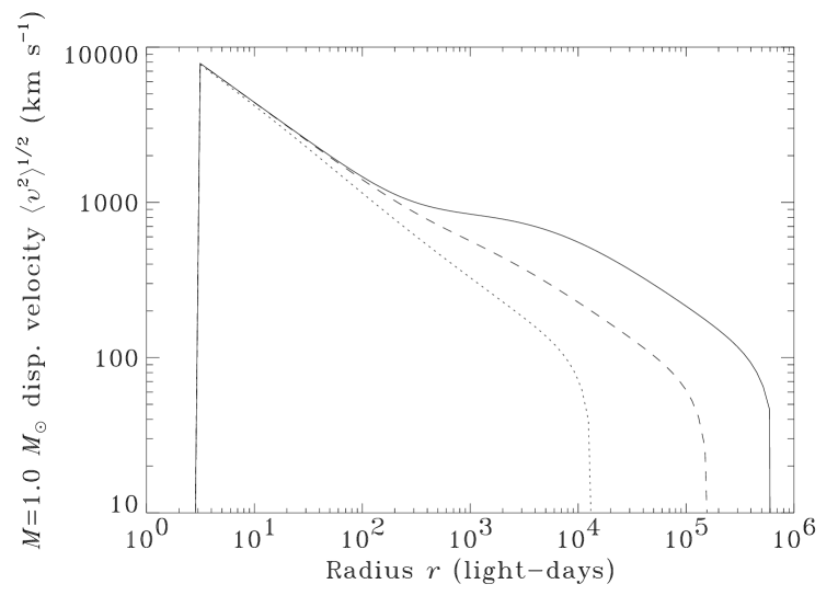
Figure 4.83: Dotted line: dispersion velocity of solar-mass stars for model 26 ($M_{\rm c}/M_{\rm h}=0.10$). Dashed line: dispersion velocity for model 27 ($M_{\rm c}/M_{\rm h}=5.0$). Solid line: dispersion velocity for model 2 ($M_{\rm c}/M_{\rm h}=50$). Note that the model 26 stellar cluster is light enough that the velocity dispersion falls as $r^{-1/2}$ everywhere.

Figure 4.83. For models with substantial narrow line covering, small variations in $M_{\rm c}$ or $r_{\rm c}$ regulate the width of the narrowest profile component. This width is simply the velocity where the log-linear profile begins to flatten. Increasing $M_{\rm c}/M_{\rm h}$ increases both this width and the overall covering in the NLR.

Most of the UV lines are less affected by the $M_{\rm c}/M_{\rm h}$ ratio than is Ly$\alpha$. This is the case, for instance, with the C IV line. As

Figure 4.84: C IV profiles for different cluster masses. Dotted line: model 26 ($M_{\rm c}/M_{\rm h}=0.10$). Dashed line: model 27 ($M_{\rm c}/M_{\rm h}=5.0$). Solid line: model 2 ($M_{\rm c}/M_{\rm h}=50$).

Figure 4.84 shows, the profile of this line is nearly the same for both the $M_{\rm c}/M_{\rm h}=5.0$ and $M_{\rm c}/M_{\rm h}=50$ models. The reason for this is simply that the line is not strong in the NLR.

As one might naively expect, the response functions at delays less than $\sim$ 100 days are even less affected by the $M_{\rm c}/M_{\rm h}$ ratio. This is shown in

Figure 4.85: Response functions of the summed line for different cluster masses. Dotted line: model 26 ($M_{\rm c}/M_{\rm h}=0.10$). Solid line: model 27 ($M_{\rm c}/M_{\rm h}=5.0$) and model 2 ($M_{\rm c}/M_{\rm h}=50$). The results are similar for each model because the $M_{\rm c}/M_{\rm h}$ parameter primarily affects only the NLR, not the BLR.

Figure 4.85 for the summed line .

Chapter 5 Summary and Discussion

We have calculated the observational features of the stellar wind model proposed by Norman & Scoville (1988) & Kazanas (1989). The main results of our study can be summarized as follows:

1. The covering function $An_{*}$ in the Kazanas (1989) model is too low and does not drop fast enough with increasing radial distance to match typical AGN line profile strengths and shapes. Using a stellar distribution function designed to be compatible with what is expected for Seyfert-class galactic nuclei, we obtain a covering factor of only 0.04. This is one-tenth the covering typically observed in Seyfert 1s. Moreover, the covering slope is very high ($d\textrm{ln}[An_{*}]/d\textrm{ln}r\simeq+0.6$), so this covering corresponds to emission from the NLR rather than the BLR (§ 4.1).

2. If the conditions in AGNs are, for poorly understood reasons, severe enough that wind mass loss rates of stars nearest to the black hole are substantially enhanced, then both the covering and its integral change. Assuming $\dot{M}\propto(L/r^{2})^{\alpha}$, where $\alpha=1.15$, we obtain a covering factor of 0.28 and a covering slope of $d\textrm{ln}(An_{*})/d\textrm{ln}r=-1.8$. The resulting optically thick area functions are approximately constant. This change results in line profile strengths and shapes similar to those in NGC 5548 (§ 4.2).

3. Though a $\chi^{2}$ fit of the various stellar wind AGN model parameters to the NGC 5548 spectral data was not performed in this study, the line ratios of model 2 are similar to those of NGC 5548. The primary reason for this is that model 2 has $\Xi=1.0$ instead of $\Xi=10$ as was originally postulated in Kazanas (1989) (§ 4.2). Even with this change, however, there were important differences between model 2 and the NGC 5548 data. For instance, the N IV $\lambda$1486 line peak is a factor of 3.7 times stronger than that in NGC 5548, while the O III] $\lambda$1664 line flux peak is a factor of 2.5 times stronger. Some of these discrepancies are probably due to the high metallicity we assumed. However, no adjustment of the abundances can resolve all of the line ratio discrepancies. In particular, Ly$\alpha$/H$\beta$, which is 20.7 in model 2, is significantly higher than the observed ratio of ratio 12.6$\pm 2.0$. This is despite the fact that the Ly$\alpha$ line in model 2 is highly suppressed by thermalization. Also, the C III]/C IV line ratios of the broad components of the profiles of our models are lower than those observed in NGC 5548. This problem arises because the continuum flux in the broad line region of NGC 5548 is so high for the distance we assumed (Krolik et al. 1991). It occurs despite our accounting for cloud/wind regions that are both angled and optically thick to continuum radiation (§§ 4.3 & 4.4).

4. The wind response functions and profiles of the stellar wind models we analyzed have a near-perfect red to blue symmetry and are not significantly shifted. Though self-absorption features were not accounted for, under the assumptions of the models they would be very weak and also not shifted (§ 2.1, Appendix K; cf Appendix L). These models, therefore, are unable to match the shifts and asymmetric response features in NGC 5548 (and other well-studied AGNs), such as the blueshift of the C III] profile peak and the difference between the C IV red and blue wing delays (§ 4.2).

5. Due to the highly asymmetric cloud line emission and an assumed optically thin intercloud BLR, our models, which for simplicity ignore local delays (cf Appendix F), yield response functions that are approximately zero at $\tau=0$ (§ 4.2). This result is different from the published response functions of NGC 5548 that probed relatively high frequencies and which yielded C IV response functions that peaked at $0\pm 2$ days (Wanders et al. 1995; Done & Krolik 1996). This difference is less severe in models in which both $r_{\rm t}$ and $M_{\rm h}$ are artificially lowered (§§ 4.13 & 4.14). However, such models have three problems. First, they have broad to narrow intensity C IV response function peak ratios of $\mathrel{\hbox{\hbox to0.0pt{\hbox{\lower 5.0pt\hbox{$\sim$}}\hss}\hbox{$>$}}}1.8$ (§ 4.2). The C IV response functions of both Wanders et al. (1995) and Done & Krolik (1996) have ratios of $\sim 1.0$. Second, such models have C IV response function FWHMs of $\mathrel{\hbox{\hbox to0.0pt{\hbox{\lower 5.0pt\hbox{$\sim$}}\hss}\hbox{$<$}}}8$ days, rather than the $\sim 15$ days suggested by observations. Third, $r_{\rm t}$ and $M_{\rm h}$ must be lowered by equal fractions to prevent the profiles from narrowing. Wind models predict a much different relation of $r_{\rm t}\propto M_{\rm h}^{1/3}$ (§ 4.14). However, since the proportionality constant in this equation is not tightly constrained in the first place, this last problem is probably not significant.

6. If $s$ is treated as a free parameter, the profile shapes suggest $s\simeq 1.7$, where $P\propto r^{-s}$. While this agrees with the Kazanas (1989) prediction of $s\simeq 2.0$, it should be pointed out that some of the line flux ratios in the $s\sim 1.0$ models we computed came closer to matching those in NGC 5548 (§ 4.5).

7. It is possible that the stellar mass functions in AGNs are “top heavy.” In this case, our calculations, which ignore winds from hot stars, may be incorrect, especially for application towards Seyfert 2s and LINERs (Appendix A). The implied IMF gradients are probably too weak to affect the covering functions significantly (Appendix B). They are, however, probably strong enough to produce severe radial dependences in the mass to light ratios (Appendix C) and high QSO metallicities (Appendix D).

8. Each of the various wind models yield specific and falsifiable predictions regarding the scaling of the response functions with the various AGN parameters. For wind models similar to model 1 (which has $\alpha-s/2\simeq-1$), we obtain $\tau_{\rm p}\propto L^{1/2}$, where $\tau_{\rm p}$ is the delay of the response function peaks (§ 4.6). Since this delay is approximately proportional to the characteristic delay of the response function, it agrees with the empirical results of Kaspi et al. (1996). Models similar to our preferred model (model 2, which has $\alpha-s/2\sim 0$) yield $\sigma_{\rm t}\propto M_{\rm h}^{1/3}$ and $\tau_{\rm p}\propto\sigma_{\rm t}$ (eq. [4.5]). This implies that the black holes masses of NLS1s are relatively low. In model 2, the tidal radius was increased by a factor of $1.8$ above the value in the CMD runs. This supports the stellar wind line emission model because this increase is much smaller than $r_{\rm t}/(3r_{\rm S})=270$, where $3r_{\rm S}$ is the only length scale common to most hypothesized AGN models with the possible exception of the pressure- and luminosity-dependent $\Xi>\Xi^{*}_{\rm c}$ one. These results suggest that measuring the correlations between $<\tau>$ and $\sigma$ in various AGNs should prove useful in testing the viabilities of the various wind models (§§ 4.13 & 4.14); reverberation studies exploring both of the $<L>$ and $M_{\rm h}$ dimensions (which, despite the obvious statistical correlation, are actually separate epoch-dependent parameters for most Seyferts) should be performed. The recent interests in NLS1s and QSO variability are good starting points in this endeavor. Future efforts to perform velocity deconvolution (Appendix J) and absorption reverberation mapping (Appendix K) will also help.

Some of the results for model 1 are similar to those found in AN94 and AN97, which also presents models of AGN line emission from stellar winds. For instance, model 1 has narrow profiles that are deficient in low-ionization broad line emission. On the other hand, our results for model 2 are different from their results. These differences arise primarily because of differences in our assumptions. We invoke a position-dependent ionization parameter in an attempt to let the stellar wind evaporation rates balance the mass loss rates (§ 3.1.1). Also, instead of permitting the reprocessing stars to have a special density function or terminal mass loss velocity, we assume that the BLR conditions are extreme enough to cause the mass loss rates to vary with radius (§ 3.1.1, Appendix B). As a result, the winds in the inner part of the BLR of our model 2 have more covering per stellar wind than those in AN94 and AN97.

From some perspectives, the stellar wind model is a failure. A basic assumption of the model, for instance, is that the wind areas increase with distance from the black hole. Such models do not appear to match observations. This failure, however, is less severe than the failures of most of the BLR models discussed in Chapter 1, which appear to have even more fundamental problems, such as violating well-established principles of physics. Moreover, the resolution of the main problems of model 1, which involved assumptions about the possible complicated interactions between the stellar winds and the hostile environment of AGNs, can be viewed more as an engineering problem than one of basic physics. From this perspective, the wind AGN model must be regarded as a viable, though, unfortunately, not simplistic solution to the AGN line emission problem. Ideally, a more complete analysis of the structure of heated winds from stars moving supersonically through the intercloud medium would be simulated using a rigorous MHD/radiative transfer code. Such an approach might answer some of the basic questions that have been raised by this study. As long as this engineering problem remains unsolved, it will probably be difficult to make firm assessments of the viability of this promising AGN model.

Appendix A UV Cross Sections of Stellar Winds for Various Stars

The first step in modeling the AGN emission line region with heated stellar winds is to determine which types of stellar winds are expected to have the largest contribution towards line emission. In this appendix, we describe why only red giant and red supergiant stellar winds were taken into account in our calculations of line emission from stellar winds in AGN.

There are two distinct possible types of line emission from stellar winds in an AGN:

1. the “reprocessed” line emission that occurs due to line cooling after heating from the UV continuum radiation and

2. the “intrinsic” line emission that would occur even without external heating from the AGN continuum source.

Reprocessed emission should be important for stellar winds which have a substantial UV cross section and which would be heated by the AGN continuum. Provided the heated wind temperature remains below $\sim 10^{5}$ K, this additional heating should be balanced by additional line emission cooling. For completeness, both reprocessed and intrinsic line emission should be included in any fully self-consistent model. However, if the stellar wind AGN model is successful at describing the BLR, the reprocessed line emission must dominate the intrinsic emission, as broad line emission in quasars and Seyfert 1s is observed to vary with the local continuum intensity. Narrow line emission, which has not yet been observed to vary with the long-term, time-averaged continuum level, does not currently have this additional constraint.

The strongest stellar winds are O-star winds. O-star winds are frequently approximated as being isothermal. The Eddington approximation for an LTE grey atmosphere yields a wind temperature of $T_{\rm{wind}}(\tau=0)=(1/2)^{1/4}T_{\rm{eff}}\sim 0.8T_{\rm{eff}}$. More detailed models indicate that temperatures in radiatively driven winds should decrease slightly with increasing radius. They also predict an ionization state of the gas that increases with radius until the effects from the interstellar medium become important. O-stars are too hot to contain neutral hydrogen and are, therefore, optically thin to UV continuum radiation near 1000 Å. Because this region of the spectrum is near the apparent AGN “big blue bump” $\nu F_{\nu}$ peak, most stellar winds should have an effective absorptive UV cross sectional area only as large as their associated radius. Thus, the situation for UV-heated O-star winds is surprisingly similar to that for UV-heated coronal winds like that of the sun.

At wavelengths below 504 and 228 Å, however, the He I and He II ionization edges give significant opacity, which can cause a hot stellar wind to be optically thick in this region. This is shown in

Figure A.1: Radius of the photosphere of a $M_{*}=34.0\,M_{\odot}$, $T_{\rm{eff}}=30,000$ K, $\dot{M}=9.6\times 10^{-7}\,M_{\odot}$ yr^-1 stellar atmosphere (solid line, left axis) as a function of photon frequency $\nu$. The dotted line is the AGN continuum assumed for the models shown in this dissertation. The dot-dashed line shows the composite AGN continuum from Zheng et al. (1997). The dashed line and right axis give the covering fraction due to this specific stellar wind. Note that, provided these models apply to O-star winds in AGN, even with 10⁶ stars of this type at a distance of 3.0 light days from the continuum source, only $\sim 1/3$ of the radiation from these continua could be absorbed. This data was kindly supplied by A. de Koter using version 3.27 of the ISA stellar wind code (e.g., Schaerer & de Koter 1997).

Figure A.1. In AGNs with continua in the BLR that are similar to the ones shown in Figure A.1, which do not have substantial EUV/soft X-ray flux, O-star winds should be unaffected by the additional AGN radiation. For this reason, and also to simplify calculations, line emission from O-star winds was neglected in this work. However, determining the actual continua in the BLR depends upon estimates of the intrinsic absorption along the line of sight. For instance, if the He I and He II column from the broad line region is high enough that the AGN spectra we observe have already been significantly absorbed below the Lyman limit, line emission from heated O-star winds would be more important than is assumed in this work. Incidentally, recent NTLE theoretical estimates of AGN accretion disk spectra do in fact predict $10^{1}-10^{2}$ times more He II ionizing photons than the older LTE accretion disk models (Hubeny & Hubeny 1997).

In contrast to stellar winds from O-stars, winds from cooler late-type stars can have a significant fractional abundance of neutral hydrogen. This permits such stars to be much more efficient at absorbing AGN continuum radiation. Therefore, in an AGN, the late-type stars should be important sources of UV line emission. Moreover, over the course of the $M\mathrel{\hbox{\hbox to0.0pt{\hbox{\lower 5.0pt\hbox{$\sim$}}\hss}\hbox{$<$}}}20\,M_{\odot}$ lifetime of a star, mass loss is greatest while in the giant phase of its evolution. This is shown in

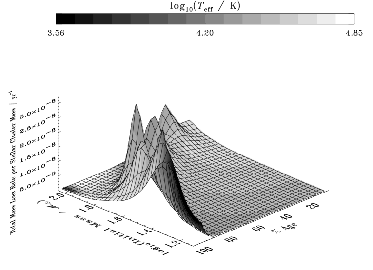
Figure A.2: Integrated stellar wind mass loss rates for massive stars as a function of scaled age and logarithm of the initial (post-Hayashi track) mass. The integrated volume under the surface is the mass loss of the stellar winds per unit stellar cluster mass. This plot is particularly useful in determining the integrated mass loss when the stellar mass density is well constrained but the stellar present day mass function is not. Under the assumptions made, injection into the interstellar medium from stellar winds is produced from stars with a wide range of initial masses, but with the heaviest stars being least important due to their sparseness. The darkness of the surface indicates the effective temperatures of the stellar photospheres. With the exception of $M>70\,M_{\odot}$ stars near the ends of their fusion-burning lifetimes, the mass loss for a given star is highest when the effective temperature is at its lowest. This is interesting because it is precisely the low-temperature winds that would have the largest UV cross sections. The effective temperature of the stars with winds that dominate the mass loss is $T_{\rm{eff}}\mathrel{\hbox{\hbox to0.0pt{\hbox{\lower 5.0pt\hbox{$\sim$}}\hss}\hbox{$<$}}}10^{4.3}$ K. This data is from Meynet et al. (1994) for mass loss rates twice the value predicted from simple photoionization codes and with $z=0.04$. The mass function index was assumed to be be $dN/dM\propto M^{-2.35}$ ($\Gamma=-1.35$) with $M_{\rm{lower}}=0.1\,M_{\odot}$, in crude accordance with Salpeter (1955).

Figure A.2. This Figure also shows that the stellar winds from O-stars are too hot to be optically thick at the $\nu F_{\nu}$ peak and the cooler winds from red giants contribute at least as much wind mass loss. For these and other reasons it was decided that our calculations would not account for line emission from O-star winds.

The mass loss rates shown in Figure A.2 are actually only valid if the mass function is similar to that of Salpeter (1955). For reasons discussed in Appendices B & C, the mass function in AGN may, however, be “top heavy,” with a higher (less negative) exponent in the stellar density distribution function. The consequences of a top heavy present day mass function upon the wind mass loss rates are shown in

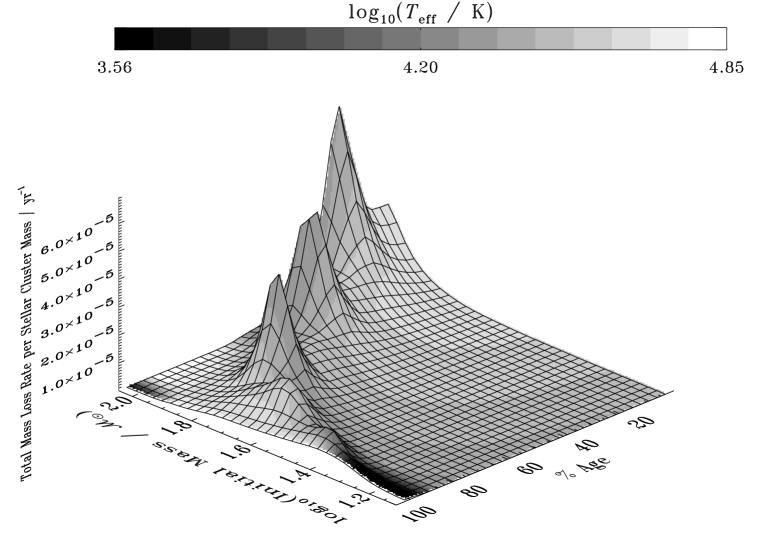
Figure A.3: The integrated stellar mass loss rates as in A.2, but under the assumptions of a very “top heavy” mass function index of -0.5. For this mass function, mass loss from $T_{\rm{eff}}\sim 10^{3.6}$ K red giants is much less than the mass loss from the warmer $T_{\rm{eff}}\sim 10^{4.3}$ supergiants. Note also that the normalization is a factor of $\sim$2000 times higher than that for the mass function assumed in Figure A.2. This is primarily due to the existence of non-plotted winds from $M<12\,M_{\odot}$ stars and $M_{\rm{lower}}=0.1\,M_{\odot}$. However, because massive stars are so much more efficient at recycling mass into the interstellar medium and their lifetimes are so short compared to solar-mass stars (see Figure A.4), a top heavy mass function still results in enhanced $M\mathrel{\hbox{\hbox to0.0pt{\hbox{\lower 5.0pt\hbox{$\sim$}}\hss}\hbox{$<$}}}10\,M_{\odot}$ mass loss rates.

Figure A.3. Not only would a top heavy mass function increase the contribution that winds of $T_{\rm{eff}}>10^{3.8}$ K stars might have upon the reprocessed line emission, but, as is shown in

Figure A.4: Integrated mass loss as a function of stellar age with overshooting for $z=0.02$. Models with enhanced post main sequence mass loss rates are shown as dotted lines. The post main sequence enhanced mass loss stars with initial masses of $M=120\,M_{\odot}$, $M=85\,M_{\odot}$, $M=60\,M_{\odot}$, and $M=40\,M_{\odot}$ each have “wind conversion efficiencies” above 90%. Data from Schaller et al. (1992).

Figure A.4, it would also increase the overall mass lost from stellar winds. In fact, one of the issues involved with the possibility of having an AGN mass function as “top heavy” as that shown in Figure A.3 is that the total mass injection rate from the winds of the cluster is several decades higher than the Eddington luminosity accretion rate. Incidentally, this is a problem only for models in which all of the mass lost from stellar winds is assumed to be accreted by the supermassive black hole—models in which, e.g., the hot, inter-cloud/stellar medium (HIM) is blown outwards into a superwind and recycled into massive stars would not suffer from this problem. Note that before massive stars become red supergiants, they would emit significant intrinsic line emission. Thus, a top heavy mass function would increase both the reprocessed and intrinsic types of stellar wind line emission. Therefore, LINERs and Seyfert 2s could simply be the result of line emission from hot stars provided $\sim$50% of galactic nuclei have very top-heavy mass functions.

In conclusion, winds from O-stars might be important contributors to AGN line emission if AGN mass functions are top heavy and the BLR soft X-ray continuum flux is high. Nevertheless, due to the current uncertainties in the present day mass function in AGN and the additional complexities/parameters involved with properly modeling warmer winds exposed to continuum radiation, we have not attempted to account for such effects—only winds from red giant stars were accounted for in our models. Future research in these areas is, however, certainly warranted.

Appendix B Comments on the Spatial Distribution of “Bloated Stars”

As discussed in §§ 3.2 and 4.12, all the observables of the stellar wind model except for the line ratios are strong functions of the particular choice of stellar density functions. In Alexander & Netzer (1994, 1997; hereafter, “AN94” & “AN97”), the winds emanating from the BLR clouds were assumed to be caused by stars “bloated” by the AGN central source. The fundamental physical properties (such as the mass loss rates) of the bloated stars were assumed to be independent of radius. The inner mass density function assumed in AN94 and AN97 is based upon the stellar densities of the models of Murphy, Cohn, & Durisen (1991; hereafter “MCD”) for $M=0.8M_{\odot}$ stars. It is $\propto r^{-1/2}$ for the first decade in radius, $\propto r^{-1}$ for the next 1.5 decades (farther out in radius), and $\propto r^{-4}$ at larger distances. In AN97, the number density of bloated stars was assumed to be two powers in $r$ steeper than the mass density function. From an observational perspective, this extra steepness affects the models in a fashion similar to the way in which a radius-dependent mass loss rate (as was essentially done in this dissertation) affects the models. It permits line profiles and response functions that agree with observational data. In this appendix, we attempt to estimate the viability of the AN97 bloated star density function. To do this, we first discuss the likely masses of bloated stars. We then discuss the theoretical and experimental indications of what the bloated star spatial densities might be in AGNs. Finally, we estimate the approximate likeliness that the relative stellar density gradients could have the magnitude and sign that were assumed in AN97. We find that this likelihood is small.

B.1 Fundamental Issues

Before addressing the question of the density function that bloated stars might have, some of their fundamental physical properties, such as their masses, must first be estimated. AN94 suggest that their bloated stars may be red giants or supergiants that have been bloated by continuum heating due to the AGN. A detailed discussion of stellar bloating is provided in § 1.2.7. Bloating can occur in the convective region of stars when the external continuum heating is sufficiently high. Kaspi et al. (1996) shows that most AGNs have luminosity-independent BLR fluxes in the range of 10⁸-10¹² ergs s^-1 cm^-2. These numbers are compatible with an AGN that has, e.g., a luminosity of 10⁴⁴ ergs s^-1, a BLR inner radius of 1 light day, and a BLR outer radius of 30 light days. According to the results discussed in Chapter 1 regarding stellar bloating, this implies that, for stars in hypothetical circular orbits in the BLR, stellar bloating could only be substantial for main sequence stars less massive than $\sim 1\,M_{\odot}$. Bloating increases the radii of the low mass stars by only $\sim$20%. The relevant time scale for this bloating to occur is the Kelvin-Helmholtz time scale of the convective envelope, which is $\sim 10^{7}$ years. As AN97 point out, the BLR stars are likely to be on highly eccentric orbits. The BLR crossing times are of the order of a year, which is much smaller than this bloating time. Therefore, the continuum flux seen by the star (in regards to any possible bloating) is the orbit-averaged flux, which is likely to be much lower than the $\mathrel{\hbox{\hbox to0.0pt{\hbox{\lower 5.0pt\hbox{$\sim$}}\hss}\hbox{$>$}}}$10¹¹ ergs s^-1 cm^-2 required to affect $M>1.0\,M_{\odot}$ main sequence stars. Note that low mass stars normally have such low mass loss rates and resultant theoretical line-emitting cross sections that even with extreme bloating they should still be insignificant contributors to AGN line emission. Thus, bloated main sequence stars are probably not good AGN line emission candidates if the heating is due to the continuum radiation.

AN94 mention that MacDonald, Stanev, & Biermann (1991) have suggested that neutrino heating might actually be the primary cause of stellar bloating. There are at least three arguments that can be made against this proposition. First, since the expected reaction pathways for high-energy neutrino production may result in a neutrino to bolometric luminosity ratio that is much smaller than unity, the effects of possible neutrino heating may intrinsically be much less important than those due to any continuum heating. Second, at least in some models, the neutrinos would not be radiated isotropically, but rather would be emitted along the jets. In this case, only a small fraction of stars could be affected. A third and more model-independent argument that could be made against neutrino-bloated stars is that for such models the covering factors should be a strong function of the neutrino luminosity. The neutrino to bolometric luminosity ratio is expected be positively correlated with the $\gamma$-ray to bolometric luminosity ratio. Approximately $\sim$10% of AGNs (only the radio-loud ones) appear to have substantial high-energy nonthermal radiation. Yet the covering factors in these objects, which presumably should have relatively high neutrino fluxes, does not appear to be significantly higher than those of the radio-quiet objects.

For the above reasons, we can probably rule out main sequence stars as bloated star candidates. This implies that bloated stars, if they exist, are (as AN94 & AN97 indeed proposed) probably late-type stars. This in turn implies $M\mathrel{\hbox{\hbox to0.0pt{\hbox{\lower 5.0pt\hbox{$\sim$}}\hss}\hbox{$>$}}}1\,M_{\odot}$, because $M\mathrel{\hbox{\hbox to0.0pt{\hbox{\lower 5.0pt\hbox{$\sim$}}\hss}\hbox{$<$}}}1\,M_{\odot}$ stars have main sequence lifetimes greater than $\sim$10¹⁰ yr. Moreover, if the bloated stars are similar to red supergiants in particular, they are “intermediate-mass” stars, with $M\mathrel{\hbox{\hbox to0.0pt{\hbox{\lower 5.0pt\hbox{$\sim$}}\hss}\hbox{$>$}}}8\,M_{\odot}$. For simplicity, we will henceforth assume this to be the case.

Because this assumed mass range is so high, bloated stars are probably very scarce. The precise shapes of the bloated star density functions are functions of the position-dependent present day mass functions in AGNs. In the next two sections we discuss some of the theoretical and empirical constraints that can be placed upon these functions and the density functions of bloated stars in particular.

B.2 Theoretical Considerations

Though the mass functions of stars in AGNs are not well known, several theoretical constraints can be made. The present day bloated star mass functions should (according to the above assumption) be proportional to the main sequence lifetime of a $M\simeq 8\,M_{\odot}$ star, which is approximately $3\times 10^{7}$ years.

The density functions are also dependent upon the particular AGN conditions. Theoretical studies by MCD indicate that there are two extreme cases to consider in AGNs regarding stellar density functions. For stellar densities significantly below $\sim 10^{7}\,M_{\odot}$ pc^-3, physical collision (also called coalescence) rates are small enough to be unimportant ($df/dt\sim 0$) compared to the loss rates due to tidal disruption. In this case, numerical work by both Bahcall & Wolf (1977) and MCD indicates that, if evolution is ignored, the intermediate-mass stars (the supergiant progenitors) follow a $n\propto r^{-7/4}$ density distribution, while the density of the lighter stars scales as $n\propto r^{-6/4}$. Incidentally, neither of these functions approaches the steepness of the $n\propto\sim r^{-10/4}$ and $n\propto\sim r^{-12/4}$ functions assumed by AN97. The reason that the massive stars have a steeper falloff is because of dynamical friction, which tends to virialize energies rather than velocities. However, the late-type red stars, which have the largest size to mass ratios, are particularly susceptible to tidal disruption. MCD show that, unlike dynamical friction, this process “flattens” the density function of the giants. Presumably, any possible bloating would enhance this process.

The other extreme case to consider is that of a density significantly above $\sim 10^{7}\,M_{\odot}$ pc^-3. For this case, MCD show that physical collisions are the leading contributor to mass loss. Because such collisions scale with the inverse power of the density squared, they also “flatten” the density distribution function of the largest stars. Since the supergiant stars have the largest cross sections, they again are the ones most subject to this process and therefore have the least steep density function in very dense stellar systems. Thus, whether or not the densities are high enough for collisions to be important in a system, it would seem unlikely that the giant stars would have a density function that falls off significantly faster than the normal populations.

One might argue that in “active” wind models, where the evolved stars are assumed to be affected by the intense continuum radiation (the “bloated stars” scenario), the situation might be different. In active stellar wind models the innermost late-type stars lose mass at an extreme rate. However, this reduces the time spent in the giant phase and hence again acts toward flattening their density function (Tout et al. 1989).

MCD included physical processes in the Fokker-Plank equation with $df/dt\neq 0$. However, they ignored several other potentially important processes that could affect the stellar densities. In particular, they ignored any possible position dependence in the initial mass function. There are several reasons that such a position dependence might exist. For instance, the Jean’s mass is

$$M_{\rm{J}}={\pi^{5/2}\rho_{0}^{-1/2}\over 6}\left(\gamma kT\over G\mu m_{\rm{p}}\right)^{3/2},$$ (B.1)

where $\rho_{0}$ is the mass density, $k$ is the Boltzmann constant, $T$ is the temperature, $m_{\rm{p}}$ is the mass of the proton, $G$ is the gravitational constant, and $\mu$ is the mass of the heaviest dust grains in the gas in units of $m_{\rm{p}}$. Temperatures near the AGN environment are probably higher than those in quiescent galactic nuclei. Therefore, equation (B.1) implies that the mean self-gravitating mass would be relatively large near AGNs. It also suggests the IMF of the massive stars has a radial dependence.

A more detailed analysis by Padoan, Nordlund, & Jones (1997) results in an upper limit to the star formation mass of

$$M_{\rm{max}}=0.2M_{\odot}\left(n\over 1\times 10^{3}\,\rm{cm}^{-3}\right)^{-1/2}\left(T\over 10\,{\rm K}\right)^{2}\left(\sigma_{v}\over 2.5\,{\rm{km}\,\rm{s}^{-1}}\right)^{-1},$$ (B.2)

where $\sigma_{v}$ is the velocity dispersion of the molecular cloud. Padoan et al. (1997) show that this expression agrees well with a Salpeter IMF for $T\sim 5-40\,\textrm{K}$. This relation has an even stronger dependence upon the temperature than that of the Jean’s mass. Padoan et al. (1997) show that a temperature of $T\mathrel{\hbox{\hbox to0.0pt{\hbox{\lower 5.0pt\hbox{$\sim$}}\hss}\hbox{$>$}}}60\,\textrm{K}$ results in “top heavy” IMFs similar to the one observed by Malumuth & Heap (1994) for R136 in 30 Doradus and starburst galaxies. Note that even with the increased temperatures associated with AGNs, extending this result to AGNs might require taking into account the higher velocity dispersions in the vicinity of a supermassive black hole. However, for the models shown in this dissertation, the gravitational influence of the black hole is overshadowed by the rest of the galaxy near and outside the NLR. Therefore, for star formation that occurs outside the BLR, the role of velocity dispersion might not be as important.

Adams & Fatuzzo (1996) derive a semi-empirical formula of

$$M_{\rm{max}}\propto{T\over\mu}^{a}$$ (B.3)

where $1\leq a\leq 3/2$. Although the assumptions Adams & Fatuzzo make are completely different than those made by Padoan et al. (1997), the final result is quite similar in that both formulas appear to predict more heavy stars near the heated AGN environment.

The innermost radius at which stars are able to form in an AGN and the associated local physical conditions such as temperature, however, are not at all known. Thus, neither the theory of Adams & Fatuzzo (1996) nor the theory of Padoan et al. (1997) appear to be robust enough to make quantitative predictions about the IMF or supergiant density function in AGNs at this time.

B.3 Empirical Considerations

One approach which bypasses some of the theoretical uncertainties discussed in the previous sections is to appeal to empirical observations. Because stars in AGNs cannot be resolved, direct measurement of the AGN mass function is not feasible. However, we can look at nearby globular clusters and galaxies in the hope that they may possess some of the same features of AGNs albeit on a much more compact scale.

If high stellar densities generally result in top-heavy IMFs, mass function gradients should exist even within the Milky Way. Massey, Johnson, & DeGioia-Eastwood (1995) measured $\Gamma$ for 18 OB associations. Their results are shown in

Figure B.1: The present-day mass function slope as a function of OB association surface density. The dashed line shows the best density-independent fit to the data, the solid line shows the best linear fit, and the dotted lines show the 1-$\sigma$ deviations in slope from the best fit.

Figure B.1. Although Massey et al. (1995) stated that there was no apparent correlation between $\Gamma$ and the local surface density, application of an F-test to their data indicates a 99.5% significance of a linear dependence. There are two differences between the analysis presented in B.1 and that shown in Figure 7 of Massey et al. (1995). First, the independent variable was assumed to be the logarithm of the surface density, rather than the surface density itself. Second, NGC 7235 was not completely removed in this analysis; the error of $\Gamma$ for this object was obtained from graphical analysis of Figure 5 of Massey et al. (1995) to be 0.9. While the results shown in Figure B.1 are suggestive of a top heavy mass function in dense regions, the relationship between surface density and position in AGNs itself is not known, so these data probably do not provide a firm means of estimating the mass function in AGNs.

Next to the galactic center, the nearest region with extremely high stellar densities is R136 in NGC 2070, which itself is in 30 Doradus. Analysis of measurements by Hunter et al. (1996) using refurbished $HST$ WFPC2 data appears to indicate a spatially dependent intermediate-mass mass function. However, the errors obtained from their methods were very large, and Hunter et al. (1996) concluded that a spatially independent intermediate-mass mass function is not ruled out. Hunter et al.’s data are shown in

Figure B.2: The mass function parameter $\Gamma$ as a function of distance from the R136 center. The dashed line is the best fit for a position-independent IMF. The solid line is the best linear fit. The dotted lines show the 1-$\sigma$ uncertainties in slope. This data is from Hunter et al. (1996).

Figure B.2. An F-test, which is insensitive to global scale factors in errors, indicates that a linear relationship is actually warranted at the 97.2% confidence level.

Figure B.3: The mass function parameter $\Gamma$ for massive stars as a function of distance from the R136 center. The dashed line is the best fit for a position-independent IMF. The solid line is the best linear fit. The dotted lines show the 1-$\sigma$ uncertainties in slope. Data from Brandl et al. (1996).

Figure B.3 shows the mass function parameter $\Gamma$ for massive stars as a function of distance from the R136 center. In this case, the slope is much higher than for the intermediate-mass stars of Figure B.2, but the significance of a linear component is not.

Presumably, the relationship between $\Gamma$ and $r$ also exists for other parameters which might more accurately reflect the local physical conditions of R136 that are responsible for the mass function gradient.

Figure B.4: As in Figure B.2, the mass function parameter $\Gamma$ for intermediate-mass stars, but as a function of mass density rather than radius.

Figure B.4 shows the result of replacing the independent variable of radius with the local mass density as inferred from the fit of Brandl et al. (1996) of the mass surface density to a standard King profile. The significance of fit is the same as the one shown in Figure B.2.

Figure B.5: As in Figure B.3, the mass function parameter $\Gamma$ for massive stars, but as a function of the local mass density.

Figure B.5 shows that such a variable transformation increases the significance of fit from 63% to 88%, which implies that for massive stars the logarithm of the local mass density has a more linear relationship with $\Gamma$ than does the logarithm of the distance from the cluster center.

B.4 A Crude Yet Quantitative Estimate of the Viability of the Bloated Star Density Assumption

We can use the results of the previous section to examine quantitatively the viability of the bloated star density function employed by AN97. If we represent the initial mass function by a simple power law, the number density per unit mass of stars more massive than $M_{\rm BS}$ is proportional to $\sim-M_{\rm BS}^{\Gamma}/\Gamma$. Combining this result with numerical differentiation of the results shown in Figure B.2 for $5M_{\odot}<M<12M_{\odot}$ stars in R136 yields an approximate bloated star logarithmic density slope enhancement of $-0.22_{-0.18}^{+0.20}$ (assuming R136 is similar to an AGN, all flattening can be ignored, etc.). This implies that a reasonable enhancement factor of the density function of bloated stars might be $r^{-0.22}$. Similarly, an enhancement of $r^{-0.42}$ would be an acceptable $-1\sigma$ deviation from this. The $r^{-2}$ enhancement factor assumed by AN97 is $-9\sigma$ below the limits implied by the R136 results. Based upon the results of the previous sections, if the bloated stars employed by AN97 were somehow less massive than 5 $M_{\odot}$, the slope enhancement probably would be smaller in magnitude. Also, relative flattening of the bloated stellar density function due to collisions and tidal disruptions was ignored in this calculation. In dense stellar systems, the flattening may be more important than gravitational friction and intrinsic IMF gradients, in which case the bloated stars may actually have the flattest density function. Thus, the $9\sigma$ deviation in amplitude result could be considered as a lower limit to the actual magnitude by which the AN97 assumption deviates from what is expected in AGNs. On the other hand, it should be pointed out that several systematic errors were not included in this calculation. Inclusion of such errors might decrease the significance of the deviation.

Incidentally, if the mass gradients implicitly assumed in AN97 were extended to the rest of the galaxy, unusual mass density functions would probably result. In particular, since the surface brightness profiles are well known, the implied stellar mass density functions could increase with galactocentric distance. Since this is highly unlikely, it is another possible problem with the AN97 models. More discussion of the relationship between stellar mass function gradient enhancements and the stellar mass functions is provided in Appendix C.

B.5 Conclusions and General Discussion

If we assume that the bloated stars in AN97 are intermediate-mass supergiants, dynamical friction and intrinsic IMF gradients may contribute to an increase in the steepness of their density functions. If the observations of R136 mass segregation are extrapolated to AGNs, the logarithmic density function slope of stars bloated by the AGN continuum flux is approximately $0.22_{-0.18}^{+0.20}$ steeper than the underlying mass function. The $r^{-2}$ density enhancement assumed by AN97 is 9$\sigma$ steeper than this. Moreover, it is likely that flattening of the density function of bloated stars due to enhanced collision and tidal disruption rates is more important than mass segregation. If this is true, the bloated star density function assumed by AN97 is even more questionable.

What is interesting about the assumption this appendix analyzes in detail is that, on the surface, it could appear to be relatively innocuous and even unimportant. This may be because the AGN system, like many others in astrophysics, is inherently complex. Thus, the theories are not well constrained. In these cases, it is actually common to introduce parameters which, when appropriately adjusted, result in reasonable fits with data. But when analyzed in more detail, the physical justification for the introduction of these parameters is often weak. The results of this appendix suggest that this is the case with the assumption regarding the density of bloated stars made in AN97.

Appendix C Extent of Mass Function Gradients and Their Implications

As discussed in Appendix B, there is some evidence that the present day mass function may vary with position (though not as strongly as implied in Alexander & Netzer [1997]). In this appendix, I discuss the possible implications of this towards our understanding of the dark matter problem.

C.1 Brief Discussion of Evidence for and Against IMF Gradients

In a recent paper, Padoan, Nordlund, & Jones (1997) claimed on theoretical grounds that the initial mass function (IMF) should be a function of the local temperature ${\it T}$ of the original molecular clouds. Padoan et al. (1997) argued that dense star forming regions, such as those in starburst galaxies, should be warmer than sparser star forming regions. In fact, if the temperature dependence of the clouds is not drastically different from that of a blackbody, then $T\propto\rho^{1/4}_{{\scriptsize\rm l}}$, where $\rho_{{\scriptsize\rm l}}$ is the local mean luminosity once star formation has already started. Padoan et al. claimed that starburst regions should therefore have a flatter IMF and be more “top heavy.” Similar reasoning would imply that the IMF in cooler regions of galaxies should favor low mass star formation and be steeper.

In support of their star formation model, Padoan et al. (1997) noted that for $T\mathrel{\hbox{\hbox to0.0pt{\hbox{\lower 5.0pt\hbox{$\sim$}}\hss}\hbox{$>$}}}60$ K, their models predict a top heavy IMF similar to that found in the center of R136 (Malumuth & Heap 1994, Brandl et al. 1996), the bright stellar cluster in 30 Doradus. Due to its proximity and the fact that it is the most massive H II region in the Local Group, 30 Doradus is perhaps the best star formation “laboratory” accessible to us. However, the relaxation time in R136 may be less than its age (Campbell et al. 1992), so dynamic friction may also contribute toward the R136 present-day mass function gradient.

Fortunately, many other avenues of testing Padoan et al.’s model exist. The O-star catalog of Garmany, Conti, & Chiosi (1982) shows a flattening of the IMF slope toward the Galactic center (cf Humphreys & McElroy 1984). This catalog also reveals a strong Wolf-Rayet/O-star ratio gradient. This supports Padoan et al.’s model since higher surface brightness regions would, on the average, yield higher temperatures and flatter IMFs. The blue-to-red O-star supergiant ratio is also a strongly decreasing function of Galactocentric distance within galaxies including the Milky Way (e.g., Hartwick 1970; Humphreys 1978). Initially, this gradient was ascribed to metallicity gradients (e.g., McClure & van den Bergh 1968). But stellar models actually predict a decrease in the blue-to-red ratio with an increase in the metallicity. (For a review of the blue-to-red gradient problem, see Langer & Maeder [1995].) As Figure A.2 shows, they also demonstrate a smooth increase in effective temperature with supergiant progenitor mass. In particular, progenitors of blue supergiants are more massive $(m\sim 40)$ than those of red supergiants $(m\sim 10)$ for a given metallicity (e.g., Schaerer et al. 1993). Therefore, the solution to this problem may simply be the existence of an IMF gradient, in which case metallicity is only a passive yet correlated variable.

Direct measurements of the IMF outside of the Milky Way are impossible for all but the nearest galaxies and indirect indicators are plagued by uncertainties in dust, metallicity, and the star formation rate. Despite these complications, several of the models which attempt to explain correlations between local surface brightness, color, line ratios, metallicity, and the star formation rate assume luminosity-dependent IMFs (e.g., Edmunds & Phillipps 1989; Phillipps, Edmunds, & Davies 1990). On the other hand, the detailed models of de Jong (1996) permit dust, metallicity, star formation rate, but not the IMF to be spatially dependent parameters. de Jong could not, however, get his models to agree with observed color gradients without also requiring them to have a very large range of metallicities in the central disk regions. Several evolutionary models of inner regions of starburst galaxies assume low mass cutoffs or top heavy IMFs (e.g., Rieke et al. 1980; Augarde & Lequeux 1985; Doane & Mathews 1993; Doyon, Joseph, & Wright 1994). Finally, independent theoretical arguments supporting IMF gradients range from models which are consistent with the simple form of the Jeans expression for the typical stellar mass in solar units of $<m>\propto T^{3/2}~{}($e.g.; Larson 1982; Bodenheimer, Tohline, & Black 1980) to much more complicated models, such as the outflow-regulated model of Adams & Fatuzzo (1996), which predicts $<m>\propto T^{a}$, where $1\leq a\leq 3/2.$

If IMFs are actually a function of $\rho_{{\scriptsize\rm l}}$ or $T$, there would be several important astrophysical consequences. For instance, there would be a position-dependence in the mean mass to light ratio. This is due to the strong dependence of the mass to light ratio upon the IMF. In R136, this makes the mass density function $\rho_{{\scriptsize\rm m}}$ much different from $\rho_{{\scriptsize\rm l}}~{}($Malumuth & Heap 1994, Brandl et al. 1996) and complicates estimates of the total mass. Padoan et al.’s results indicate that similar effects might occur in spiral galaxies. If the luminosity of a star is taken as $L\simeq L_{\odot}m^{y}$, where $y\simeq 3.5,$ the Jeans expression above would suggest the crude relation $<m>\propto\rho^{3/8}_{{\scriptsize\rm l}}$ and yield $\rho_{{\scriptsize\rm m}}\propto\rho^{1+3(1-y)/8}_{{\scriptsize\rm l}}\simeq\rho^{0.06}_{{\scriptsize\rm l}}$. Unfortunately, previous works have assumed that IMFs are independent of time and position with, specifically, $\rho_{{\scriptsize\rm m}}\propto\rho^{1.0}_{{\scriptsize\rm l}}$ throughout a given spiral galaxy (e.g., van Albada et al. 1985). In this appendix, surface mass densities of spiral galaxies are computed, for the first time, by explicitly accounting for the possible types of IMF gradients that might exist if theories like those of Padoan et al. are correct.

C.2 An Empirical Estimate of the R136 IMF Gradient

Since position-dependent measurements in R136 of both $\rho_{{\scriptsize\rm l}}$ and the IMF slope $\Gamma$ (where ${\it dN}/{\it dM\propto m}^{\Gamma-1}$ is the number of stars per unit mass in solar units) have already been made, computing the dependence of the R136 IMF upon the local luminosity is straightforward. Doing this will provide a useful starting point in obtaining a crude yet quantitative estimate of the possible types of IMF gradients that might generally exist in all galaxies including the Milky Way.

Table C.1: IMFs in R136

$R$/pc	$\Gamma(R)$	$m_{\rm l}$	$m_{\rm u}$	$\rho_{\rm l}/(L_{\odot}{\rm pc}^{-3})$
0.20	$-1.29\pm 0.20$	5.6	120	$1.5\times 10^{6}$
0.60	$-1.46\pm 0.23$	3.6	76	$1.5\times 10^{5}$
2.0	$-2.12\pm 0.09$	$\leq 2.0$	48	$1.5\times 10^{3}$

Data adapted from Brandl et al. (1996) for (age-spread restricted) stars 2.5—3.5 Myr old.

Table C.1 summarizes Brandl et al.’s (1996) results for the IMF based upon high resolution 5-color photometry of the stars in R136 estimated to be between 2.5 and 3.5 Myrs years old. The right-most entry of Table C.1 shows the results of performing the coordinate transformation between ${\it R}$ and $\rho_{{\scriptsize\rm l}}$ using Figure 15 of Hunter et al. (1996). Though Brandl et al. (1996) did not make explicit measurements of the upper and lower stellar mass cutoffs $m_{{\scriptsize\rm l}}$ and $m_{{\scriptsize\rm u}}$ to the power-law approximation of the IMF, Table C.1 includes estimates of their dependences upon the local surface brightness. The lower mass limits were obtained from the peaks of Brandl et al.’s mass functions, while the upper limits were taken from the highest masses observed per radius bin. Both $\log_{10}(m_{{\scriptsize\rm l}})$ and $\log_{10}(m_{{\scriptsize\rm u}})$ are found to decrease by $\simeq 0.2$ with each successive increase in radius. Brandl et al. (1996) performed completeness corrections, so the depletion of low mass stars in all but the outer regions of R136 is presumably real. The results of performing a linear fit of the IMF parameters of R136 to $\log_{10}(\rho_{{\scriptsize\rm l}})$ are shown in columns 2-7 of Table C.2 as Model A. Uncertainties of parameters calculated from more than two radius bins are shown in parenthesis.

Table C.2: Model Parameters

Model	$\Gamma_{0}$	$\Gamma_{1}$	$m_{\rm l0}$	$m_{\rm l1}$	$m_{\rm u0}$	$m_{\rm u1}$	$\rho_{\rm m\odot}/$	$\Sigma_{\rm m\odot}/$	$<\Sigma_{\rm m\odot}>/$
							$M_{\odot}{\rm pc}^{-3}$	$M_{\odot}{\rm pc}^{-2}$	$M_{\odot}{\rm pc}^{-2}$
A	$-3.03$	$0.28$	$-0.08$	$0.13$	$1.25$	$0.12$	0.12	67	67
	$(\pm 0.26)$	$(\pm 0.06)$	$\ldots$	$\ldots$	$(\pm 0.23)$	$(\pm 0.04)$	…	…	…
B	-1.11	0.42	-1.52	0.00	1.30	0.00	0.31	179	179
C	-0.55	0.40	-1.52	0.00	1.60	0.00	0.10	60	195

This assumes $f=f_{0}+f_{1}{\rm log}_{10}[\rho_{\rm l}/(L_{\odot}{\rm pc}^{-3})]$, for $f=\Gamma$, ${\rm log}_{10}(m_{\rm l})$, or ${\rm log}_{10}(m_{\rm u})$.

C.3 Dynamical Properties of Spiral Galaxies with IMF Gradients

The IMF gradient of Model A implies a surface mass density that is different from what would be obtained were the mass to light ratio constant. The surface mass density for Model A, if scaled according to the surface luminosity function suspected for the Galaxy, is shown in the top panel of Figure C.1. The disk scale length $R_{0}=4.5$ kpc and solar Galactocentric radius $R_{\odot}=7.8$ kpc were taken from Kuijken & Gilmore’s (1989a) model of the Galaxy. For simplicity, $\rho_{{\scriptsize\rm l}}$ at a given radius was assumed to be constant throughout a disk thickness of 575 pc. The surface brightness was normalized to be $22.5~{}L_{\odot}$pc^-2 at $R=R_{\odot}$, which results in $\rho_{{\scriptsize\rm l\odot}}\equiv\rho_{{\scriptsize\rm l}}(R_{\odot})=0.037~{}L_{\odot}$pc^-3. For each radius bin, the IMF was obtained from $\rho_{{\scriptsize\rm l}}$ and the coefficients shown in Table C.2 for Model A. This IMF was converted to present day mass and luminosity functions by assuming (purely for simplicity) a constant star formation rate for the past $1.0\times 10^{10}$ yrs. The main sequence lifetime-luminosity-mass relationships used to obtain the mass to light ratio as a function of the IMF were obtained from logarithmic-linear interpolation of $m\geq 0.8$ models published by Schaller et al. (1992) for $z=0.02,$ overshooting of the $m\geq 1.5$ stars, and standard mass loss rates. For $m<0.8,L|_{m=0.25}=7.8\times 10^{-4}L_{\odot},~{}L|_{m=0.08}=6.55\times 10^{-9}L_{\odot}$, and $L|_{m\leq 0.07}=5.0\times 10^{-12}L_{\odot}$ were assumed.

The surface densities both of Model A and of the constant mass to light ratio model fall off exponentially with increasing radius. The effective scale length of Model A is $\simeq 7.5$ kpc, which is $\simeq 1.7$ times larger than that of the surface brightness function. This increase in the scale length is a result of the fraction of low mass stars (and the mass to light ratio) increasing with radius.

From the surface density, other dynamical properties of the galaxy can also be calculated. The circular velocity (i.e., the rotation curve) corresponding to the surface density of Model A is shown in the upper middle panel of

Figure C.1: Top panel: the surface density of a spiral galaxy similar to the Milky Way but with the IMF of Model A. The dotted line is the surface density assuming that all stars lie on the main-sequence. The dashed line is the surface density if the V band mass to light ratio were constant at $\gamma_{{\scriptsize\rm V}}=2.0M_{\odot}/L_{\odot}$. Lower three panels: circular velocities of Models A (upper middle), B (lower middle), and C (bottom). The circular velocities of Model A correspond to the surface density function shown in the top panel. For each model, the solid curve accounts for all components of mass, the dot-dashed curve accounts for just the halo, the dotted curve accounts for just the disk, the short-dashed curve accounts for just the bulge and spheroid stars, the dash-triple-dotted curve accounts for everything except the halo, and the long-dashed curve represents a model with a constant mass to light ratio of $\gamma_{{\scriptsize\rm V}}=2.0M_{\odot}/L_{\odot}$. The thicknesses of the disks were ignored in these computations. At ${\it R<}0.30$ kpc, the gravitational force in Model A due to the disk-bound mass is outward. The corresponding value of the circular velocity is technically imaginary, but is plotted here as negative. A similar but opposite effect occurs at the outer edge of the disk, which is at 35.0 kpc in these models, where the circular velocities level off or even rise just before following nearly Keplerian motion.

Figure C.1. The parameters for the bulge, spheroid, and halo were taken from Table C.1 and Figure 5 of Kuijken & Gilmore’s (1989a) model of the Galaxy. To avoid a divergent and unphysical total mass, the additional assumption that all components of the Galaxy terminate at an arbitrarily selected maximum radius of 35.0 kpc was also made. For Model A, this results in a total mass of the halo, bulge/spheroid, and disk of, respectively, $2.8\times 10^{11}M_{\odot},3.5\times 10^{10}M_{\odot}$, and $6.3\times 10^{10}M_{\odot}$. In comparison, the integrated disk mass of the $\gamma_{{\scriptsize\rm V}}=2.0M_{\odot}/L_{\odot}$ model is only $3.2\times 10^{10}M_{\odot}$ and increases much faster with radius. Similar results were obtained using the Bahcall & Soniera (1984) Galaxy model, though their smaller disk scale length of 3.5kpc causes the intermediate regions of the disk to have a higher density. For simplicity, the surface mass density of stellar remnants and gas was assumed throughout the disk to be 1/3 that of the stars. Because the halo dominates the mass distribution, the circular velocity curve (solid line) is nearly flat. Without the halo, the circular velocity curve falls from 185 km s^-1 at $R=2.0$ kpc to 124 km s^-1 at $R=34$ kpc. Though the surface density of Model A corrected for IMF gradients is different from that previously obtained for spiral galaxies, Figure C.1 shows that the change is not enough to dramatically affect the dynamical properties of the disk, such as the circular velocity curve.

Another, more direct, effect of Model A’s IMF gradient is shown in

Figure C.2: The IMF of Model A at a Galactocentric radius of 1.0 kpc (dotted line), 7.8 kpc (solid line), and 15 kpc (dashed line). Though the differences between these three IMFs are small in terms of parameters traditionally computed from IMFs, they correspond to large differences in the mass to light ratios.

Figure C.2. For numerical reasons, the slopes at $m<m_{{\scriptsize\rm l}}$ and $m>m_{{\scriptsize\rm u}}$ were set, respectively, to be $\Gamma=+3$ and $\Gamma=-8$ rather than positive and negative infinity. The IMF of Model A is very negative at all radii, with $\Gamma|_{R=1.0\hbox{~{}{\scriptsize\rm kpc}}}=-3.2,\Gamma|_{R=R_{\odot}}=-3.4,$ and $\Gamma|_{R=15.0\hbox{~{}{\scriptsize\rm kpc}}}=-3.6.$ This occurs even though R136’s spatially averaged IMF is typical and its IMF gradient is small only because it has a luminosity density that is $\sim 10^{4}-10^{8}$ times higher than typical regions of spiral galaxies. For comparison, Salpeter (1955) found $\Gamma=-1.35$ for $0.4\leq m\leq 10,$ while Miller & Scalo (1979) obtained much higher values of $\Gamma=-0.4,-1.5,$ and -2.3 for, respectively, $0.1<m<1.0,1.0<m<10,$ and $m>10.$

These differences suggest that the IMFs in R136 and the Milky Way do not directly scale to one another via the $\rho_{{\scriptsize\rm l}}$ variable. This may be because R136 has recently experienced its first starburst. In this case, a better correlation variable to employ might be $<\rho_{l}>_{t}$, the time-averaged luminosity density. It may also be because of other inherent differences between R136 and the Milky Way. For instance, the bright, early-type stars in spiral galaxies are generally confined to relatively narrow Galactocentric radii near that of their initial birth sites. In contrast, stars in elliptical galaxies similar to R136 undergo substantial mixing due to their highly eccentric orbits. At any rate, the IMFs in spirals like the Milky Way may scale differently than the scaling in R136.

For these reasons, other models were also considered. Model B was constructed in order to help answer the question of just how necessary the dark halo is for circular velocity curves to be flat. The IMF gradient $\Gamma_{1}$ was adjusted to minimize the curvature of the outer circular velocity curve, while $\Gamma_{0}$ was adjusted such that the rotation velocity was $\simeq 220$ km s^-1. For simplicity, $m_{{\scriptsize\rm l}}$ and $m_{{\scriptsize\rm u}}$ were fixed. The lower middle panel of Figure C.1 shows that the circular velocity curve of Model B is surprisingly flat throughout most of the outer regions of the disk before the halo component is included. The total disk mass for Model B is $2.4\times 10^{11}M_{\odot}$, with $<\gamma_{{\scriptsize\rm v}}>_{\hbox{{\scriptsize\rm disk}}}{\scriptsize\rm=}14.5M_{\odot}/L_{\odot}$, which is 7.3 times larger than the $\gamma_{{\scriptsize\rm V}}=2.0M_{\odot}/L_{\odot}$ model. The value of $\Gamma_{1}$ for Model B is 0.42. This is $50\%$ higher than the IMF gradient in R136. The change within the Milky Way of $\Gamma$ measured by Garmany et al. (1982) between the inner and outer semicircular regions of radius 2.5 kpc surrounding the Sun was -0.8, which for a disk scale length of $R_{0}=4.5$ kpc corresponds to $\Gamma_{1}=0.8\times 3\pi R_{0}/(8$loge$\times 2.5$ kpc)=3.9. This is much higher than the value in Model B. Thus, the IMF gradient of Model B is well below empirical constraints.

However, there are at least five potential problems with the halo-less form of Model B:

1. In the adopted solar vicinity $(R_{\odot}=7.8$ kpc), the surface density is $179M_{\odot}$pc^-2. This is an unacceptable 15 standard deviations higher than the local value of $46\pm 9~{}M_{\odot}$pc^-2 measured by Kuijken & Gilmore (1989b). The corresponding mass to light ratio is $7.9M_{\odot}/L_{\odot}$. This is $60\%$ higher than the local value adopted in standard texts such as Binney & Tremaine (1987). Similarly, the IMF slope at this radius is $\Gamma=-1.7.$ For the low mass $(m\mathrel{\hbox{\hbox to0.0pt{\hbox{\lower 5.0pt\hbox{$\sim$}}\hss}\hbox{$<$}}}0.5)$ stars, this value is incompatible with Miller & Scalo’s (1979) result of $\Gamma=-0.4.$

2. Mestelian disks, which are similar to Model B, are commonly thought to be unstable to bar formation. The Toomre instability parameter $Q$ is $\sigma_{R}\kappa/(2.9G\Sigma_{{\scriptsize\rm m\odot}})$, where $\kappa\simeq 36$ km s^-1 kpc^-1 is the epicycle frequency and $\sigma_{R}$ is the mass-weighted stellar velocity dispersion (Toomre 1974). Published estimates are $Q\simeq 1-3$ in the solar vicinity. Because stellar velocity dispersions are empirically observed to decrease with mass even for stars with lifetimes greater than the age of the Galaxy, estimates of $\sigma_{R}$ are sensitive to $m_{{\scriptsize\rm l}}$. Wielen (1977) obtained $\sigma_{R}=62\pm 12$ km s^-1 for $0.1\mathrel{\hbox{\hbox to0.0pt{\hbox{\lower 5.0pt\hbox{$\sim$}}\hss}\hbox{$<$}}}m\mathrel{\hbox{\hbox to0.0pt{\hbox{\lower 5.0pt\hbox{$\sim$}}\hss}\hbox{$<$}}}0.8$ K and M dwarfs, which implies $Q\mathrel{\hbox{\hbox to0.0pt{\hbox{\lower 5.0pt\hbox{$\sim$}}\hss}\hbox{$>$}}}1.0\pm 0.2$ for Model B. This lower limit is low enough to sustain spiral arm structure which numerical simulations show would rapidly dissipate otherwise. However, it is too near unity to prevent the growth of substantial arm/interarm stellar mass density contrasts. Though such mass contrasts are now known to exist in normal spirals (e.g., Rix & Zaritsky 1995, González & Graham 1996), they are not accounted for in Model B. Incidentally, the halo component does not necessarily affect this instability (Sellwood 1985).

3. The circular velocity curve at $R\mathrel{\hbox{\hbox to0.0pt{\hbox{\lower 5.0pt\hbox{$\sim$}}\hss}\hbox{$<$}}}35$ kpc is not precisely flat, but actually rises before attaining a nearly Keplerian fall off. This is the result of the non-spherical potential.

4. The circular velocity drops below 200 km s^-1 in the inner regions of the disk. This result is expected. For Model B, the mass to light ratio is

   $$\simeq m^{1-y}_{{\scriptsize\rm u}}(m_{{\scriptsize\rm u}}/m_{{\scriptsize\rm l}})^{-\Gamma-1}(y+\Gamma)(M_{\odot}/L_{\odot})/(-\Gamma-1),$$ (C.1)

   where $L\propto m^{y}$ is assumed for $m\mathrel{\hbox{\hbox to0.0pt{\hbox{\lower 5.0pt\hbox{$\sim$}}\hss}\hbox{$<$}}}m_{{\scriptsize\rm u}}$. If

   $$\Gamma_{1}=[\ln(m_{{\scriptsize\rm u}}/m_{{\scriptsize\rm l}})\log_{10}{\it e}]^{-1},$$ (C.2)

   which Model B obeys to within $15\%$, the mass to light ratio would scale as $\simeq e^{R/R_{0}}$. This in turn would imply a disk surface density that is relatively constant. The circular velocities of such disks increase monotonically with $R$ and are zero at $R=0.$ This problem with low inner disk velocities is probably not serious because circular velocity curves are frequently compatible even with constant mass to light ratio, halo-less models throughout their entire optically bright regions (e.g., Kent 1986). Furthermore, flatter, halo-less velocity curves could probably be attained by including the following: galaxy parameters slightly different than those of Kuijken & Gilmore (1989a), a (more realistic$)\log$-normal IMF (Miller & Scalo 1979), expected spatial dependence in remnant and gas mass fractions, and variations of $m_{{\scriptsize\rm l}}$ or $m_{{\scriptsize\rm u}}$ with $\rho_{{\scriptsize\rm l}}$. For instance, the velocity dip is better masked by the bulge if Bahcall & Soniera’s (1984) smaller disk scale length of 3.5 kpc is assumed.

5. The IMF gradient of Model B appears to be too small to be compatible with the measurement of Garmany et al. (1982). Equation (C.2) suggests that this discrepancy would be less if a smaller $m_{{\scriptsize\rm u}}/m_{{\scriptsize\rm l}}$ ratio had been employed.

Of the above potential problems, only the first two appear to be significant at this time. Both can be overcome by taking into account the arm/interarm density contrasts observed in spiral galaxies; Model C was constructed to be similar to Model B, but has an azimuthally averaged light and mass density that is 3.25 times greater than the interarm values in which the Sun presumably resides. The circular velocity curve of Model C, shown in the lower panel of Figure C.1, is slightly higher, but otherwise similar to that of Model B. However, the solar-vicinity disk surface density is only $60M_{\odot}$pc^-2. This is a much more reasonable 1.6 standard deviations above the value determined by Kuijken & Gilmore (1989b) and is actually lower than Bahcall & Soniera’s (1984) value of $\simeq 85M_{\odot}$pc^-2.

C.4 Discussion

A direct scaling of R136’s IMF to the Galaxy does not dramatically alter the circular velocity curve. However, Models B and C, with their higher, yet modest IMF gradients, have nearly flat $v_{\hbox{{\scriptsize\rm circ}}}\mathrel{\hbox{\hbox to0.0pt{\hbox{\lower 5.0pt\hbox{$\sim$}}\hss}\hbox{$<$}}}220$ km s^-1 circular velocity curves only before the traditional dark halo component is included. Note that if one assumes that these types of models and their $\sim 10^{1}$-fold mass enhancements are representative of most galaxies, that the fiducial stellar contribution towards the closure density is $\Omega_{*}\simeq 0.004~{}($e.g., Peebles 1993) before accounting for IMF gradients, that the cosmological constant is zero, and that there is no hot dark matter, one would obtain

$$\Omega\simeq\Omega_{\hbox{{\scriptsize\rm baryon}}}\simeq 0.04+\Omega_{\hbox{{\scriptsize\rm gas}}}.$$ (C.3)

In this equation, $0.007\mathrel{\hbox{\hbox to0.0pt{\hbox{\lower 5.0pt\hbox{$\sim$}}\hss}\hbox{$<$}}}\Omega_{\hbox{{\scriptsize\rm gas}}}$$\mathrel{\hbox{\hbox to0.0pt{\hbox{\lower 5.0pt\hbox{$\sim$}}\hss}\hbox{$<$}}}0.08~{}($Mulchaey et al. 1996), where $\Omega_{\hbox{{\scriptsize\rm gas}}}$ is the closure fraction due to all gas including hot plasma in galactic clusters.

Current models of galactic evolution (e.g., Dwek 1998, Worthey $1994,\&$ de Jong 1996) do not account for IMFs that might vary with time and position via the temperature. This is true despite prior warnings that the IMF probably has important dependences upon time and position (e.g., Mihalas & Binney 1978). In light of the above results, accounting for IMFs with such dependences may be necessary even to obtain results that are only accurate to first order. Accounting for these dependences may, for relatively obvious reasons, clarify our understanding of several astrophysical phenomena including the G-dwarf problem, intrinsic (as a function of radius) and extrinsic (as a function of galactic morphology) metallicity and color gradients, and the Tully-Fisher relation.

However, some problems remain with assuming that the above models are even representative of spiral galaxies. For instance, why would the disk-edge peaks of Models B and C not have been observed? Also, why would spiral galaxies conspire to obey a relation similar to equation (C.2)? Questions similar to these will be addressed in future work.

Appendix D Obtaining AGN Abundances from Galactic Abundance Gradients and the [O/Fe] Ratio

D.1 Introduction

Abundances in AGNs are generally estimated by analyzing spectral features like line ratios. Some of these estimates have yielded extremely unusual abundances. For instance, Marshall et al. (1993) obtained results that yield [O/Fe]$\mathrel{\hbox{\hbox to0.0pt{\hbox{\lower 5.0pt\hbox{$\sim$}}\hss}\hbox{$<$}}}-0.9$ in active galaxy NGC 1068, where $[\textrm{X}/\textrm{H}]$ is defined to be $\log\left(A\left(\textrm{X}\right)/A_{\odot}\left(\textrm{X}\right)\right)$, $A(\textrm{X})$ is the abundance of element X, and $A_{\odot}(\textrm{X})$ is the solar abundance of X.

As universal as the general procedure employed by Marshall et al. (1993) towards determining abundances is, it has some important shortcomings. For instance, the method requires knowledge of the curves of growth associated with the lines, which in turn depend upon opacities, which themselves generally depend upon the physical conditions of the line-emitting gas. The equivalent width of an absorption feature is, for example, proportional to the elemental abundance if the clouds are small enough and if other conditions are such that a line is optically thin. However, it is equivalent to the square root of the abundance if the cloud geometry and other conditions are such that the line is saturated. Unfortunately, since most of the physical conditions like this are only poorly constrained in AGNs, estimates of abundances in AGNs have important systematic errors in addition to the well-understood random ones. In fact, Marshall et al. (1993) speculate that their abundance estimates might be incorrect due to the potentially incorrect values of the iron opacities they assumed in their calculation. For these reasons, an independent means of estimating AGN abundances which bypass the problems with the traditional method would be desirable. In this appendix, I describe and employ a new method for obtaining abundances in AGNs which, though currently very crude, does precisely this.

D.2 Procedure

This new method takes advantage of the fact that essentially all metals are formed in stars. It is for this reason that abundances are a direct function of the time- and position-dependent stellar birthrates, IMFs, and stellar evolution characteristics. In this appendix let us assume that these functions are closely coupled to the mean stellar luminosity density averaged over the life of the galaxy (as opposed to the luminosity density that might exist during a starburst). This assumption is similar to that made in Appendix C. It specifically implies

$$[\textrm{X}/\textrm{H}]=[\textrm{X}/\textrm{H}]_{0}+[\textrm{X}/\textrm{H}]_{1}\log\left(\rho_{\rm l}/\rho_{\rm l\odot}\right).$$ (D.1)

In the above equation, $\rho_{\rm l}$ is intrinsic luminosity density and the other three variables on the right hand side are free parameters. In this appendix, we will attempt to extrapolate the abundance gradients in the Milky Way to other galaxies. In this case, provided we neglect the fact that the sun is more enriched than its neighbors, $\rho_{\rm l\odot}$ can be taken as the luminosity density in the solar vicinity, $[\textrm{X}/\textrm{H}]_{0}$ can be assumed to be zero, and $[\textrm{X}/\textrm{H}]_{1}$ specifies the abundance gradient. Note that the subscripts “0” and “1” placed on $[\textrm{X}/\textrm{H}]$ are not to be confused with an occasionally used means of denoting different observational measurement techniques.

For a hypothetical bulge-less spiral galaxy, the dynamic range in $\rho_{\rm l}$ is relatively small. This is because at $R\ll R_{0}$ the luminosity density is approximately constant. In an AGN, however, $\rho_{\rm l}$ continues to increase at $R\ll R_{0}$, so equation (D.1) would yield drastically larger inner disk to outer disk metallicity ratios. However, in very bright regions, one would expect that the star formation rate is limited by negative feedback. For this reason, the value of $[\textrm{X}/\textrm{H}]_{1}$ in active galaxies may be lower than the value in the solar vicinity. To determine whether or not this is the case, $[\textrm{X}/\textrm{H}]_{1}$ could in principle be directly computed using current galactic evolutionary models. However, such a calculation is far beyond the scope of this appendix and would probably be poorly constrained anyway due to various free parameters.

Here I simply assume that $[\textrm{X}/\textrm{H}]_{1}$ is the same for all galaxies and estimate it for the Milky Way from the radial metallicity gradients observed in H II regions, supernova remnants, planetary nebulae, and stars. Assuming $\rho_{\rm l}=\rho_{\rm l0}e^{-R/R_{0}}$ for the Galaxy, we have

$$[\textrm{X}/\textrm{H}]_{1}=-\frac{R_{0}/\textrm{kpc}}{\log e}\frac{d[\textrm{X}/\textrm{H}]}{d(R/\textrm{kpc})}.$$ (D.2)

D.3 Results

Equation (D.2) yields the luminosity-dependent abundances of He and S shown in

Figure D.1: Middle dotted line: abundance estimate of He as a function of mean local luminosity density according to equation (D.1) and Table 1 of Peimbert (1992). Outside dotted lines show 1$\sigma$ observational errors ignoring the potentially large systematic uncertainties of equation (D.1). Dashed lines: abundance and 1$\sigma$ errors of S. Solid (vertical) lines: lower and upper boundaries of the luminosity densities that may be appropriate for NGC 5548. Regions to the left of the left horizontal line have stellar densities that are much lower than those near AGNs, while regions to the right of the right horizontal line are not be realized due to mixing and other factors. Asterisk: the actual abundance employed in the computer runs shown in Chapter 4, assuming the density luminosity at $r=1.0\,\textrm{pc}$ in model 1.

Figure D.1. Because stellar orbits are suspected of being highly eccentric below $\sim$1 pc (see, e.g., Appendix B), mixing should be dramatically enhanced in this range, which would reduce any abundance gradients in this very small region. For this reason, the upper limit to the luminosity density relevant to equation (D.1) was adopted to be that at $r=1.0\,\textrm{pc}$ in model 1 (which is described in Chapters 3 and 4). The lower limit to the luminosity density was assumed to be the luminosity density at $r=10\,\textrm{pc}$, approximately where the radial covering function attains its maximum value in model 2. In these calculations, a mass to light ratio of 10 $M_{\odot}/L_{\odot}$ was adopted. This number is also not well constrained, and other ratios are clearly possible. The abundance gradients $d[\textrm{X}/\textrm{H}]/(dR/\textrm{kpc})$ were obtained by statistically averaging results shown in Peimbert (1992), Friel & Janes (1993) (for Fe only), and Panagia & Tosi (1981) (for Fe only). For simplicity, solar abundances at Galactocentric radius $R=R_{\odot}=7.8\,\textrm{kpc}$ (not to be confused with the solar radius) were assumed, giving $[\textrm{X}/\textrm{H}]_{0}=0$. The scale radius $R_{0}$ was taken to be $4.5\textrm{ kpc}$, while the axially averaged luminosity density (see Appendix C) at $R=R_{\odot}$ was taken to be $\rho_{l\odot}=3\times 0.039\,L_{\odot}\,\textrm{pc}^{-3}$.

Figure D.1 suggests, based upon what we know about the evolution of the Galaxy, that metallicities in AGNs could be extremely high. This is not to say that they are definitely this high, as there are far too many fundamental systematic uncertainties (ignored physical effects) associated with equation (D.1). In fact, this is the reason that it was decided to employ near solar abundances in our models. But very high AGN metallicities would certainly not be in conflict with the metallicity gradients that are observed in the Galaxy, especially if the IMF is top-heavy in these extreme environments.

Figure D.2: Dotted lines: abundance and $1\sigma$ error estimates of C. Dashed lines: abundances and $1\sigma$ error estimates of N. Other lines and data points are as in Figure D.1.

Figure D.2 shows the abundance estimates for C and N, while

Figure D.3: Dotted lines: abundance and $1\sigma$ error estimates of O. Dashed lines: abundances and $1\sigma$ error estimates of Fe. Other lines and data points are as in Figure D.1.

Figure D.3 shows the abundance estimates of O and Fe. These plots suggest that C, N, O, and Fe abundances in AGNs may indeed be extremely high.

Figure D.4: Solid line: projected [O/Fe] as a function of luminosity density. shows just [O/Fe] without errors. Dotted horizontal line: upper limit of [O/Fe] in the AGN NGC 1068 according to Marshall et al. (1993). Other lines and datum point are labelled as in Figure D.1.

Figure D.4 shows the projected values of just the [O/Fe] ratio. They suggest that A(Fe/O) should be enhanced in AGNs by an order of magnitude or more.

Taking this “what-if” scenario associated with equation (D.1) one step farther, the lower limit to the luminosity density in NGC 1068 relevant to equation (D.1) can be very crudely estimated from the intersection point of the lines in D.4, yielding $\rho_{\rm l}\mathrel{\hbox{\hbox to0.0pt{\hbox{\lower 5.0pt\hbox{$\sim$}}\hss}\hbox{$>$}}}2\times 10^{4}\,L_{\odot}\,\textrm{pc}^{-3}$. This luminosity density is well within reasonable limits. The beauty of what we have done here is that there has been no need to resort to “exotic” physics, such as drastic changes in iron opacities or sub-solar AGN O abundances (Marshall et al. 1993).

D.4 Discussion

So far, we have explored the empirical side of metallicity gradients. We have found that the Galactic metallicity gradients are compatible with the observed AGN abundances. An obvious question to ask is whether or not these results are fully consistent with various theoretical predictions. Interestingly, they may not be.

It is generally believed that Fe is predominantly produced by Type Ia supernovae and that O is predominantly produced by Type II supernovae. This belief arises in part from the observed supernovae spectral line ratios. It also arises from current models (e.g., Tsujimoto et al. 1995), in which the majority of Fe produced in Type II supernovae is imploded rather than exploded. This results in traditional Type II supernovae models yielding a flat or even decreasing Fe yield as progenitor mass increases. The same is not expected for O, which is synthesized at stellar radii larger than that of the Fe.

The potential problem stems from the fact that, for the reasons discussed in Appendix C, IMFs probably become relatively top-heavy IMF toward galactic centers. Since the progenitor masses of Type IIs are higher than the progenitor masses of Type Ias, one may expect higher, rather than lower, O/Fe abundance ratios towards the Galactic center.

This suggests that one or more of the following is true:

1. The ratio of Type Ia to Type II supernovae increases towards the Galactic center despite indications of IMF gradients. This could be due to, for example, the binary fraction decreasing with Galactocentric radius.

2. The Fe yield estimates of high-mass Type II supernovae are too low.

3. The present measurements of the Fe/O abundance Galactic gradient are incorrect, the Marshall et al. (1993) result is an anomaly, and/or the IMF gradients and mechanisms for metal production assumed in this chapter (e.g., eq. [D.1]) are incorrect.

Though possibility (1) is perhaps most likely, possibility (2) should not be ruled out. This is because possibility (2) primarily involves the tweaking of theoretical parameters not well established in the first place, like the radii of the implosion/explosion boundaries in current one-dimensional models, which may be smaller for high-mass supernovae progenitors than current estimates. Some of the indications that current theoretical supernovae models may be inadequate is the ¹³⁸Ba overabundance observed in SN 1987A, which is a factor of 2.5 greater than theoretical upper limits (Mazzali & Chugai 1995). Also, recent Type Ic “hypernovae” SN 1998bw (Iwamoto et al. 1998) produced 0.7$M_{\odot}$ of Fe precursor ⁵⁶Ni. This yield exceeds traditional theoretical upper limits by about one order of magnitude.

Finally, it is worth discussing an additional implication of equation (D.1) towards AGN luminosities. Equation (D.1) predicts that the metallicity in observable AGNs increases with redshift. This is simply because higher luminosity AGNs probably have higher maximum effective values of $\rho_{\rm l}$. Physically, this makes sense according to the results of Appendixes B and C which imply that the stars in the high-luminosity AGNs are more massive than those in the Milky Way. This should result in much more efficient ISM enrichment. Note that the lifetimes of massive stars (which are the underlying time scales for enrichment of these systems) are extremely short compared to the age of the universe. Therefore, since higher redshifts correspond to higher luminosities for a flux-limited survey, AGN metallicities should (despite some claims to the contrary) appear to increase with redshift. According to results of Hamann & Ferland (1992), this appears to indeed be the case.

Appendix E Does the Intercloud Medium Pressure Affect the Stellar Wind Shape?

For simplicity, the stellar winds in the models we present in Chapter 4 are assumed to be spherically symmetric. In this appendix, I briefly discuss the validity of this assumption if there is an intercloud medium.

The problem of a stellar wind moving through a homogeneous medium at high velocity has been already addressed by, e.g., Brighenti & D’Ercole (1995). The situation is quite similar to that of colliding winds in binaries (e.g., Cooke, Fabian, & Pringle 1978) and, to a lesser extent, comet tails (e.g., Beard 1981). There are probably five basic physical parameters of relevance: the terminal stellar wind velocity $v_{\infty}$ on the “shocked side” of the star, the velocity of the star through the intercloud medium $v_{*}$, the mass loss rate of the star $\dot{M}$, the intercloud density mass density $\rho_{\rm{HIM}}$, and the speed of sound of the intercloud medium $v_{\rm{s}}$.

If $v_{*}\gg v_{\rm{s}}$, these parameters can probably be orthogonalized into a mere two of essential importance: the Mach number $M\equiv v_{*}/v_{\rm{s}}$ and the stand off distance of the shock to the star $l$. This stand off distance in front of the stars is the place where the wind momentum flux balances the intercepted intercloud momentum flux,

$$l=\left(\frac{\dot{M}v_{\infty}}{4\pi\rho_{\rm{HIM}}v^{2}_{*}}\right)^{1/2}.$$ (E.1)

In the general vicinity of the star, the approximate shape of the shock front for an $M\gg 1$ wind should be spherical directly in front of the star and conical farther away such that the angle of the shock surface normal to the stellar velocity vector is $\leq\tan^{-1}(1/M)$.

Of interest here is just the question of spherical symmetry. In particular, if $l\gg R_{\rm w}$, the line-emitting sections of the stellar winds are clearly emitted from a region inside the shock front that is still spherically symmetric. Otherwise, they may not be, and the models in Chapter 4 should probably be re-run using a more sophisticated code capable of accounting for the asymmetries.

A key variable of equation (E.1), $\rho_{\rm{HIM}}$, has not yet been reliably measured. Nevertheless, one can obtain potential upper limits to $\rho_{\rm{HIM}}$ in a variety of ways. One upper limit, for instance, is the value of $\rho_{\rm{HIM}}$ which would result in the heating through drag (as the stars travel through the intercloud medium) being comparable to or higher than the ordinary heating from the continuum. As shown in Figure 1.6, these two sources of power become comparable when the intercloud medium pressure is similar to the expected cloud edge pressure. Another upper limit to $\rho_{\rm{HIM}}$ is that which would result in Fe K-shell photoelectric absorption, which does not appear to be significant in most AGNs. Mathews & Ferland (1987) showed that if a BLR size of 10¹⁹ cm is assumed and the HIM is in pressure equilibrium with BLR clouds that have edge densities of 10^9.5 cm^-3 , the intercloud medium temperature required for lack of the Fe K-shell absorption edges is greater than 10^8.7 K. A more modern estimate might assume a BLR radius of 10 light days (2.6$\times$10¹⁶ cm) and a BLR cloud edge density of 10¹⁰ cm^-3, which would yield an HIM temperature of above 10^7.2 K. Since this temperature is near the Compton temperature expected in AGNs, the upper limit is similar to that obtained with an intercloud medium that has the same pressure as the wind/cloud edges.

This upper limit gives the lower limit to $l$ shown in

Figure E.1: Solid line: minimum stand off distance $l_{\rm{min}}$ to wind size $R_{\rm{w}}$ ratio assuming $T_{\rm{HIM}}=10^{7}\,\textrm{K}$ and equal HIM and wind edge pressures for model 2. Dotted line: ratio for model 1. If $l\gg R_{\rm{w}}$, the line-emitting regions of the clouds should be unaffected by ram pressure. These results imply (yet by no means prove) that this might not be the case.

Figure E.1 assuming $T_{\rm{HIM}}=10^{7}\,\textrm{K}$ and a mean molecular weight per HIM particle of 1.3$m_{\rm p}$. This upper limit to $\rho_{\rm{HIM}}$ results in $l_{\rm{min}}<R_{\rm{w}}$ throughout the BLR. Incidentally, as

Figure E.2: Solid line: approximate Mach number $M$ for the intercloud protons of model 2 if the intercloud medium temperature is 10⁷ K. Dotted line: the approximate Mach number for protons of model 1 under the same assumptions.

Figure E.2 shows, the stars in this model move supersonically throughout the BLR. These results suggest that nonspherical effects due to the HIM could be important, particularly in low-$v_{\infty}$ models, such as the ones of AN94 and AN97.

However, as argued in Kazanas (1989), a feature of the wind models is that they, unlike the pressure-equilibrium cloud models, do not require the existence of any intercloud medium in the first place. Moreover, as is discussed in Appendix L, nonspherical models would require at least one additional parameter to characterize the unknown physical properties of the intercloud medium in the BLR. For these reasons, it was decided to not include nonspherical effects in the code for the runs shown in Chapter 4. But this does not by any means imply that this should not be done in future wind models, particularly if a measurement of the BLR intercloud medium density is obtained which yields $l\mathrel{\hbox{\hbox to0.0pt{\hbox{\lower 5.0pt\hbox{$\sim$}}\hss}\hbox{$<$}}}R_{\rm w}$.

Appendix F Local Delays

In Chapter 2 we assumed that the emission characteristics of illuminated clouds are purely a function of the instant continuum flux to which they are exposed. In this appendix, I analyze the validity of this assumption. I find that this universally adopted assumption may be wrong, and that the history of exposure accounting for “local delays” due to finite cloud equilibrium times may also be relevant. In such cases, I show that the mean response time is a function of the recent average value of the continuum. I also show that if instantaneous or linear response is incorrectly assumed, local delays and nonlinear response can make a system appear larger than its actual size. Finally, I show that local delays can be a source of asymmetry about the peak of the cross-correlation function.

F.1 Background

Procedures for computing a linearized response function of the time-dependent line emission given off from an ensemble of clouds illuminated by a time-dependent source are well known (e.g., Blandford & McKee 1982). They assume that the contribution toward line emission from a specific source is purely a function of the radius from the central object and the instantaneous continuum flux to which it is subjected. This requires that the processes relevant to its line emission attain equilibrium much more quickly than the other time scales involved. The explicit time-dependent response of individual clouds, where, e.g., the line emission efficiency in a cloud lags the continuum flux it experiences, has not yet been accounted for in previous works concerning AGN variability.

Accounting for finite equilibrium times, however, can yield interesting results for most of the AGN cloud models that have been proposed. Consider, for instance, a cloud model in which the cloud area is a decreasing function of the cloud pressure, which is externally regulated by the pressure of an intercloud medium. Rees, Netzer, & Ferland (1989) additionally assumed $P\propto r^{-s}$, where $P$ is the pressure throughout the cloud and $r$ is the distance from the black hole. Let us consider the analogous case where the pressure is regulated by the local ionizing continuum flux $F_{{\scriptsize\rm c}}$ and only indirectly through $r$, namely $P\propto F^{s/2}_{{\scriptsize\rm c}}$. Such a dependence implies that a change in the continuum luminosity invokes a change in the cloud pressure as well. As we shall see, “reactive” cloud models like this one offer both theoretical and empirical advantages over static ones. Note that the clouds would not react instantaneously; a minimum for the characteristic time scale for internal pressure equilibrium to be asymptotically obtained is the sound crossing time of the clouds. As noted in Netzer (1990), this time scale can be similar to the continuum variation time scales, suggesting that clouds of this model rarely might be in actual pressure equilibrium. Therefore, even though the outermost layer emitting a line can be a small fraction of the cloud as a whole, clouds of this model should to some extent “remember” their prior pressures and areas.

Because line emission from clouds is a strong function of the area, pressure, and pressure ionization parameter $\Xi~{}($defined here as the ionizing photon to gas pressure), the line efficiency of a cloud has a nontrivial time dependence. For instance, consider the case where the continuum flux local to a cloud suddenly increases. If $s<2,$ the pressure ionization parameter of the cloud would at first follow the increase in the continuum flux, but would then decrease as the pressure begins to approach its new equilibrium value. Relative to Ly$\alpha$, the flux in a line like N ${\scriptsize\rm v~{}\lambda}1240,$ which is probably a relatively high ionization transition in stable cloud sections (Taylor 1994), would initially rise, but then decay as the ionization parameter decreases. The response function that one would obtain upon a linear fitting would have structure not only at the range of lags corresponding to the light crossing times of the emission region, but also at lags greater than these by the pressure equilibrium times in the clouds.

In such a case, the previous works on AGN variability, which have all assumed that a response function at a given lag is proportional to the density of clouds along the corresponding “iso-delay” surface, are inapplicable. Specifically, the results based upon equation (2.13) of Blandford & McKee (1982), which was derived under the assumption that the equilibrium time scales of the cloud properties are all much less than the light crossing time (hereafter, the “fast cloud” assumption), are now suspect. This is an important point because a great deal of effort has been expended to obtain and analyze variability data using the approach of Blandford & McKee (1982).

In § F.2 of this appendix we find that there are several cloud properties affecting line emission that could be strong functions of the local continuum flux with equilibrium times large enough to violate the fast cloud assumption. Because, for these cases, the popular formalism of Blandford & McKee (1982) is invalid, a new and more general formalism for analyzing variability data will be developed in § F.3. This new formalism is compatible with models that have clouds with finite equilibrium times and nonlinear responses. Readers not interested in the mathematical derivation of the time-dependent line profile with the new formalism may wish to skip to § F.4, where the new theory is applied to some simple models. A summary is provided in § F.5.

F.2 Motivation

In order for the formalism of Blandford & McKee (1982) to be invalid for a given cloud model, two conditions must be satisfied for at least one of the cloud properties in the model. The first of these conditions is that the line emissivity be a moderately strong function of the cloud property and that the cloud property in turn be a moderately strong function of the local continuum flux a cloud experiences. The second condition is that the equilibrium time scale of the cloud property be near one of the other characteristic time scales of the system. If the equilibrium time scale is near or greater than the line emission region light crossing time, the response function will be affected. Conversely, if the equilibrium time is near the time for clouds to cross the emission region, the time-averaged line profile can be affected. Determining the precise way in which the response functions and profiles are affected requires a detailed and highly model-dependent analysis. Before going through such an analysis, let us first discuss some of the cloud line emission model properties which apparently meet the above two conditions.

Table F.1 lists some of the processes responsible for reactive cloud properties in several of the models that have been proposed and the equilibrium time scales associated with them. Also shown is whether the slowness of equilibrium affects the response functions, line profiles, or line ratios. The first entry is for a two-phase pressure-equilibrium model (e.g., Wolfe 1974; Krolik, McKee, & Tarter 1981). Assuming in this case that the cloud pressure is regulated by pressure of the intercloud medium, the delay in the cloud pressure response to the continuum is limited by the intercloud temperature equilibrium time scale. For the model parameters described in Table F.1, this is (only) $\simeq 43$ days. If the dependence of the intercloud temperature upon the local continuum flux is strong enough, the responding pressure will affect the response functions for the parameters assumed in Table F.1 in a highly line-dependent fashion, giving the line ratios a complicated time dependence. Furthermore, if the cloud identities are preserved (as in Rees, Netzer, & Ferland 1989), the slowness of the cloud area and column density reactions will also affect the response functions respectively in a line-independent and weakly line-dependent fashion. The time-averaged line profiles for this model are not affected by the finite pressure equilibrium time, which is too small compared to the cloud crossing time $(\sim 2$ years for the parameters shown in Table F.1) to be affected. However, if the intercloud temperature dependence is moderately strong, this model, like several others that are not immune to the various processes analyzed in Table F.1, requires use of a new formalism. Such a formalism will be developed in § F.3.

Table F.1: Equilibrium Processes of Some Reactive Cloud Model Parameters and Their Effects

Name of Limiting	Cloud	Parameter	Observational
Process	Parameters	Equilibrium	Parameters
	Affected	Times	Affected
Inter-cloud Cooling1	$A,N_{{\scriptsize\rm c}},P_{l}$	43 days	RF, LR (strong)
Thermal Evaporation2	$A,N_{{\scriptsize\rm c}},P_{l}$	20 years	RF, LP, LR (strong)
Pressure-limited Evaporation3	$A,N_{{\scriptsize\rm c}}$	2.0 days	RF, LR (weak)
Pressure-limited Evaporation3,4	$P_{l}$	$\sim 0.37$ days	RF, LR (strong)
Stellar Wind Expansion5	$A,N_{{\scriptsize\rm c}},P_{l}$	20 days	RF, LR (strong)
Stellar Photospheric Heating6	$A,N_{{\scriptsize\rm c}},P_{l}$	$10^{-2}-10^{11}$ days	RF, LP, LR (strong)
Magnetic Confinement7	$A,N_{{\scriptsize\rm c}},P_{l}$	4.3 days	RF, LR (strong)

NOTE—“RF,” “LP,” and “LR” are respective abbreviations for “response functions,” “line profiles,” and “line ratios.” These results are for clouds at a fiducial radius from the continuum source $r_{0}$ of 10 light-days (the light crossing time scale), a fiducial local continuum flux of $10^{44}/(4\pi r^{2}_{0})$ ergs cm^-2, a fiducial velocity of 4000 km s^-1, a fiducial cloud hydrogen density of $10^{11}$ cm^-3, and a fiducial mean column density of $10^{22.5}$ cm^-2.

¹Only for models with clouds in pressure equilibrium with a hot inter-cloud medium (e.g., Krolik, McKee, & Tarter 1981). Calculation assumes an inter-cloud temperature of $10^{7}$ K, which implies that the dominant source of cooling is thermal Bremsstrahlung, which in turn implies flux-dependent (reactive) cloud parameters.

²Adopted from results in Krinsky and Puetter (1992), but after scaling to the column density assumed here. Line ratios are only strongly affected for pressure-stratified clouds.

³Only for pressure-stratified cloud models, see Taylor (1994).

⁴Only for lines emitted uniformly from the inverse-Strömgren region.

⁵Adopted from parameters assumed in Schaaf & Schmutzler (1992).

⁶Adapted from Harpaz & Rappaport (1991) and Antona & Ergma (1993).

⁷As in Rees (1987), but assuming the field responds to the continuum flux on the Alvén wave cloud crossing time.

Note that the physical processes considered in Table F.1 were drawn from the set of processes invoked by the various cloud models that have been proposed. In principle, all of these could be incorrect. Therefore, Table F.1 is necessarily incomplete. For this reason, the analysis of time-dependent cloud response could be important even if all of the processes in Table F.1 somehow accommodated the fast cloud assumption.

F.3 Theory of Response

In this section we shall extend the formalism in Blandford & McKee (1982) so that information can be obtained from variability data about models which violate two fundamental assumptions made in Blandford & McKee (1982): (1) instantaneous response and (2) linear response.

F.3.1 Locally Delayed Response

Before one can understand the overall, global response of systems that can violate the fast cloud assumption, one must first understand the response of the individual clouds that make up such systems. In this section a general method of determining the time dependence of an arbitrary cloud property is derived. In § F.3.2, this method will be used to obtain the global response of systems that can violate the fast cloud assumption.

The character of the response of an AGN cloud depends critically upon the relative magnitude of two time scales. One of these is the variation time scale of some condition externally imposed upon the cloud, such as the local continuum flux or intercloud pressure. Another is the characteristic equilibrium time scale of a physical property of the cloud, such as its temperature or size, in response to the variations of the external conditions. As an example, let us consider the case of a cloud with a physical property that is an increasing function of the local continuum flux. Let us also assume, for this example, that the continuum source, itself, is time-independent, but that the cloud is in a periodic orbit about the black hole. This situation is a simple variation on those in which the continuum does vary. If we assume that the orbital period is significantly greater than the equilibrium time scale of the property, the physical property would lag the time-averaged continuum flux to which the cloud is exposed as it orbits the black hole. The line emission in such a cloud would depend not only on its position, but also on another variable which indicates its orbital phase. Under certain conditions (see Appendix G), it can be shown that this variable can be the cloud velocity vector. For instance, if the line emissivity of a cloud is an increasing function of just the physical property, then the line emission from the cloud would be greatest not when it is closest to the black hole, but slightly farther away, after the cloud has acquired a small outward velocity. As the orbital time becomes even larger, we approach the “fast cloud” regime. In this regime we can assume that the physical property in the cloud reacts fast enough that it is purely a function of the local flux or, in this case, of the distance from the black hole such that the phase lag is zero.

A second case to consider is one wherein the variation time scale of the local continuum flux of a cloud is significantly smaller than the equilibrium time of the property. Here the physical property of the gas would lag the orbital motion by a significant phase. This implies that a line with a strong enough dependence upon the lagged property could attain maximum flux when the cloud has a relatively high outward radial velocity. In this case, as the variation time scale of the input continuum flux becomes even smaller, we approach the “slow cloud” regime, where we can simply assume that the relevant physical property is a constant throughout the orbit.

The third possible case to consider is one in which the local continuum variation time scale is intermediate and similar to the equilibrium time scale. Understanding this case requires a more quantitative approach than the other two cases. Let us call the generic cloud property of interest $y(t)$ where ${\it t}$ is the time measured in the reference frame of the observer. The analysis which follows is quite general and $y(t)$ could represent properties such as the mean cloud area, pressure, or column density. Similarly, let $x(t)$ be a generic input, such as the local continuum flux near the cloud, of which $y(t)$ is assumed to be a function. Let $y^{\prime}(x)$ be the asymptotic functional dependence of $y$ upon $x$ once sufficient time has elapsed for equilibrium to be established, where the prime denotes the functional dependence in the fast cloud regime. Furthermore, let us assume that there exists a characteristic time scale $\tau_{y}$ for $y$ to respond to changes in x. Such a characteristic time will be equal to the ratio of the extent to which $y$ is out of equilibrium to the rate at which the non-instantaneously responding component of $y$ actually attains its equilibrium value. This gives

$$\tau_{y}={y^{\prime}{\hbox{\bf(}}x(t){\hbox{\bf)}}-y(t)\over\dot{y}(t)-\dot{x}(t)\tilde{\hat{\Psi}}_{y|x}(\infty)<y>/<x>},$$ (F.1)

where $\tilde{\hat{\Psi}}_{y|x}(\infty)$ is a free parameter that is the instantaneous component of the “gain” of $y$ with respect to ${\it x}$, and $<x>$ is the average or “bias” of ${\it x}$, etc. The gain itself is an operator (defined by eq. [H.3]) that yields the dimensionless ratio of the amplitudes of small variations of an output about its mean with respect to that of some input. It is merely the Fourier transform of the linearized response function (see Appendix B). The implicit assumption here that $\tau_{y}(x)$ is approximately constant could be invalid under the following conditions: the variations of $x$ are large enough, the initial conditions are far enough from equilibrium, or the equilibrium time has an explicit dependence upon the sign of $\dot{x}(t)$. In these cases the physics associated with the response time is not properly described by only one parameter. Otherwise, equation (F.1) completely characterizes the system given the prior inputs $x(t^{\prime}\leq t)$ and the other system characteristics $y^{\prime}(x),\tau_{y}$, and $\tilde{\hat{\Psi}}_{y|x}(\infty)$.

Though we will assume that $y^{\prime}(x)$ is a nonlinear function, in certain instances we shall find it highly instructive to consider the case in which the variations in $x$ are small enough that $y^{\prime}(x)$ is accurately described by a first-order Taylor expansion. Performing such linearization of equation (F.1) (with eqs. [H.1]-[H.4]) yields in the frequency domain

$$\tilde{\hat{\Psi}}_{y|x}(\omega)={\eta(y|x)+i\tilde{\hat{\Psi}}_{y|x}(\infty)\tau_{y}\omega\over 1+i\tau_{y}\omega},$$ (F.2)

where $\omega_{y}\equiv 1/\tau_{y}$ and $\eta(y|x)\equiv\tilde{\hat{\Psi}}_{y|x}(0)$ is the “asymptotic gain” of $y$ with respect to ${\it x~{}}($see also eq. [H.2]). Equation (F.2) can be used to formulate a more precise definition of the fast and slow cloud regimes, which respectively occur for $\omega\ll\omega_{y}$ and $\omega\gg\omega_{y}$, where the transfer function becomes a trivial function of $\omega~{}($flat in $\log-\log$ coordinates).

Equation (F.2) yields in the time domain

$$\hat{\Psi}_{y|x}(\tau)=\tilde{\hat{\Psi}}_{y|x}(\infty)\delta(\tau)+\Theta(\tau)[\eta(y|x)-\tilde{\hat{\Psi}}_{y|x}(\infty)]\omega_{y}e^{-\tau\omega_{y}},$$ (F.3)

where $\Theta$ is the step function. This response function tells us (namely via eq. [H.6]) the contribution in the linear regime toward the output (e.g., the cloud area) made by an input (e.g., the local continuum flux [measured in the reference frame of the cloud]) at a prior time. The first term in equation (F.3) is the component of $y$ that mirrors the variations in ${\it x}$ without delay, while the second term is the component of $y$ that responds on the time scale $\tau_{y}$.

For the important case in which the instantaneous component of the gain is zero, equations (F.2)-(F.3) yield the results indicated earlier in this section: in the fast cloud regime they yield an output that mirrors the input variations, while in the slow cloud regime they yield an output that is constant.

F.3.2 The Line Profile

Now that we have prescribed a general way of accounting for individual cloud properties that exhibit hysteresis-like behavior, we can derive the more observable properties of AGN models which have finite (rather than zero) equilibrium times. Of particular interest here is the angle-dependent apparent luminosity $L^{{\scriptsize\rm cl}}_{l}$ emitted in line $l$ of a cloud with position vector from the black hole ${\bf r}$ and velocity vector ${\bf v}$. An expression for this that is general enough for the models that will be analyzed in this appendix and which takes local delays into account is

$$L^{{\scriptsize\rm cl}}_{l}(t,{\bf r},{\bf v},\hat{{\bf s}})=F_{{\scriptsize\rm c}}(t,{\bf r})A\epsilon_{l}[1+\epsilon_{\hbox{{\scriptsize\rm A}{\scriptsize\it l}}}\hat{{\bf r}}\cdot\hat{{\bf s}}]+L^{{\scriptsize\rm s}}_{l},$$ (F.4)

where $F_{{\scriptsize\rm c}}(t,{\bf r})$ is the ionizing continuum flux at ${\bf r}$, A is the cloud area, $\epsilon_{l}$ is the dimensionless emission efficiency for line $l,~{}\epsilon_{\hbox{{\scriptsize\rm A}{\scriptsize\it l}}}$ is the first-moment correction to the efficiency for an anisotropically emitting cloud, ${\bf D}\equiv{\bf r}+{\bf s}$ is the position vector of the observer, and $L^{{\scriptsize\rm s}}_{l}$ is the cloud luminosity in line $l$ due to resonance scattering. Each of the cloud parameters in equation (F.4) that has an equilibrium time near or greater than $r/c~{}($hereafter, the “spatial time” scale) must be evaluated using the appropriate form of equations (F.3) and (H.6). Before a model conforming to equation (F.4) can have predictive power, not only must the continuum light curve be measured, but also estimates of the time scales and the asymptotic functional dependence of each cloud parameter upon the local continuum flux must be made.

Once a specific expression for the observed line flux from an individual cloud is assumed, the macroscopic characteristics of the global system composed of several clouds are easy to calculate. Neglecting absorption, the flux per cloud observable at ${\bf D}$ is $F^{{\scriptsize\rm cl}}_{l}(t,{\bf r},{\bf v};{\bf D})\propto L^{{\scriptsize\rm cl}}_{l}(t-s/c,{\bf r},{\bf v},\hat{{\bf s}})/s^{2}$. With this terminology, the time-dependent line profile becomes (see Appendix G)

$$F_{l}(t,v_{D})=\int d^{3}rd^{3}vf({\bf r},{\bf v})F^{{\scriptsize\rm cl}}_{l}(t,{\bf r},{\bf v};{\bf D})\delta(v_{D}+{\bf v}\cdot\hat{{\bf D}}),$$ (F.5)

where $v_{D}$ is the equivalent tangential velocity and $f$ is the distribution function. Under the conditions specified earlier, the above equation permits computation of the line profile for any class of AGN cloud line emission models which can be described by equation (F.4).

Though equation (F.5) provides a means of computing the nonlinear line profile response when the input history is known, applying it can be computationally expensive (though not as much as the trajectory-dependent sum method considered in Appendix G). This is because it requires modeling the cloud properties such as the $F^{{\scriptsize\rm cl}}_{l}$ function, which from a numerical perspective is an array with dimensions ${\bf r}$ and ${\bf v}$ that evolves with time, though probably only weakly in the ${\bf v}$ dimensions. If local delays are important, evaluation of $F^{{\scriptsize\rm cl}}_{l}$ at each point in time requires integrating over history according to the appropriate forms of equation (H.6). Since the positional integral in the above equation can be interpreted as an integral over history, the expression for the line profile is a double integration over lag. This is in contrast to the analogous expression for the line profile given by equation (2.12) of Blandford & McKee (1982), which involves only a single integration over lag.

F.3.3 The Line Transfer Function and Linear Approximation of the Line Profile

By linearizing equation (F.4) (see Appendix B), one of the integrations in lag in equation (F.5) can be eliminated, and the computer time required to obtain the time-dependent line profile of a model can be significantly reduced. For several key cases, we find that these benefits outweigh the inaccuracy of linear models.

The first step in linearizing the line flux emitted from an individual cloud is to obtain its gain about the bias continuum flux. This in turn requires determining the transfer function (eq. [F.2]) of each flux-dependent cloud parameter affecting the line emission in equation (F.4). Because the gain is calculated by considering small perturbations about the mean of the input, the gain of each of these parameters can be computed using the time-averaged local continuum flux, which is dependent only upon position. In terms of the gains of these cloud parameters, equation (F.4) yields for an individual cloud

$$\tilde{\hat{\Psi}}_{L^{{\scriptsize\rm cl}}_{l}|F_{{\scriptsize\rm c}}}(\omega;{\bf r},{\bf v},\hat{{\bf s}})=1+\tilde{\hat{\Psi}}_{A|F_{{\scriptsize\rm c}}}(\omega)+\tilde{\hat{\Psi}}_{\epsilon_{l}|F_{{\scriptsize\rm c}}}(\omega)+{<\epsilon_{\hbox{{\scriptsize\rm A}{\scriptsize\it l}}}>\hat{{\bf r}}\cdot\hat{{\bf s}}\over 1+<\epsilon_{\hbox{{\scriptsize\rm A}{\scriptsize\it l}}}>\hat{{\bf r}}\cdot\hat{{\bf s}}}\tilde{\hat{\Psi}}_{\epsilon_{\hbox{{\scriptsize\rm A}{\scriptsize\it l}}}|F_{{\scriptsize\rm c}}}(\omega)+\tilde{\hat{\Psi}}_{L^{{\scriptsize\rm s}}_{l}|F_{{\scriptsize\rm c}}}(\omega),$$ (F.6)

where we will implicitly assume that the continuum flux is evaluated locally (at ${\bf r})$. Each of the above terms is proportional to the gain of one of the reactive cloud parameters. The third term itself is the sum of three highly model-dependent terms if $\epsilon_{l}=\epsilon_{l}(\Xi,P,N_{{\scriptsize\rm c}})$ sufficiently parameterizes the cloud emission for a given model. Note that even if the various cloud properties such as the area are described without approximation by a nontrivial linear response function, the output line response in a cloud is nonlinear nonetheless. This is because the above equation provides only an approximation to the response valid for small perturbations about a mean. Such nonlinearity is a general property of reactive cloud models.

With each cloud response linearized, the remaining time dependence in the system line flux equation is due purely from the $F_{{\scriptsize\rm c}}$ factor, so the global transfer function of the profile is

$$\tilde{\hat{\Psi}}_{F_{l}|F_{{\scriptsize\rm c}}}(\omega;v_{D})=\int d^{3}rd^{3}v{<F^{{\scriptsize\rm cl}}_{l}(t,{\bf r},{\bf v};{\bf D})>_{t}\over<F_{l}>}f({\bf r},{\bf v})\tilde{\hat{\Psi}}_{F^{{\scriptsize\rm cl}}_{l}|F_{{\scriptsize\rm c}}}(\omega;{\bf r},{\bf v},\hat{{\bf s}})\times$$

$$e^{-i\omega(\hat{{\bf r}}-\hat{{\bf D}})\cdot{\bf r}/c}\delta(v_{D}+{\bf v}\cdot\hat{{\bf D}}).$$ (F.7)

The line flux gain of an individual cloud appearing in this equation is equal to the gain of the individual line luminosity (eq. [F.6]) if, for the time being, we neglect absorption. Note that unlike the Fourier transform of the expression given for the response function by Blandford & McKee (1982), the above equation has a factor of the cloud gain that can be nonzero at nonzero frequency. In the time domain, equation (F.7) gives (via eq. [H.6]) the linear approximation to the line profile flux,

$$F_{l}(t,v_{D})=<F_{l}(t,v_{D})>_{t}\left[1+\int d\tau\left({F_{{\scriptsize\rm c}}(\tau-t)\over<F_{{\scriptsize\rm c}}>}-1\right)\hat{\Psi}_{F_{l}|F_{{\scriptsize\rm c}}}(\tau;v_{D})\right]\pm\sigma_{F_{l}},$$ (F.8)

where $\sigma_{F_{l}}$ represents the input-dependent error. Unlike equation (F.5), this equation does not have an implicit nested integration in lag. Applications of it to the models considered in this appendix that account for the dependence of $F^{{\scriptsize\rm cl}}_{l}$ upon the direction of the velocity vector are provided elsewhere (Taylor 1994).

It is worth repeating that a condition for the linearized response function to be descriptive is that at a given radius the continuum variations are small enough that the second order derivatives can be neglected. Since large-scale variations in the continuum luminosity are known to occur, the system would be somewhat contrived to consistently obey this condition. For instance, in the slow cloud regime the linearized form of equation (F.6) will generally be inaccurate at low enough mean cloud ionization parameters when the emitting ion is in partial fractional abundance. In this case, the second derivative of $\epsilon_{l}$ with respect to $F_{{\scriptsize\rm c}}$ would not only be large and positive for most lines, but would also be a sensitive function of input level. If the asymptotic mean cloud ionization parameter is a decreasing function of the local flux $(s<2~{}[$§ F.1]), overestimates for the size of the line emission region when using fully linear models are implied. Even for wind cloud models (e.g., Kazanas 1989) in the fast cloud regime with $s=2,$ where the effective ionization parameter can be taken to be constant, nonlinearities would still arise from the dependence of the cloud area upon flux for which a constant $\eta(A|F_{{\scriptsize\rm c}})$ term cannot account. In any of these types of situations, the Fourier transform of the oscillatory component of the line flux would not be proportional to that of the continuum, and forms of equation (F.8) would not accurately describe the variability that would be observed.

In such cases, the “optimal” response function that best fits real data becomes a function of both the specific data set as well as the fitting criterion (see also eqs. [H.12]-[H.13]). Therefore, its utility in measuring any of the epoch-independent features of AGN and AGN models is somewhat questionable. This is in contrast with the linearized response function (eq. [F.7]), which is dependent upon only the mean of the continuum flux. Ideally, a fitting criteria would exist that would reliably yield this input-independent, poorly fitting linearized response function rather than the optimal one. However, there are alternative parameters and parameterized functions for analyses of variability data that completely bypass this problem. One alternative is the cross-correlation function. However, even in the linear regime this is also a strong function of the excitation characteristics. (See also § F.4.) A more promising alternative is to fit nonlinear models (e.g., eq. [H.8]; Taylor & Kazanas 1992) to data. Using nonlinear models offers the potential of epoch-independent fitting or measurement within the context of a model of physical AGN properties even when the continuum variations are large or the line emission is a sensitive function of the flux.

F.4 Examples

Let us consider cloud models in which the effective reprocessing efficiencies are increasing functions of the local continuum flux, with the equilibrium time scale of the relevant physical properties being slightly larger than the characteristic light crossing time. From § F.3, we know that responses to short and weak pulses of continuum radiation in such a system could be modeled satisfactorily with a linear “spatial” response function, which is the response function of the system were the fast cloud regime applicable. This response function has structure on just the light crossing times of the emission region, as the efficiency and physical conditions of the clouds in such a system would deviate only slightly from their mean values. Similarly, responses to long pulses of fixed intensity probably also could be mimicked with a different linear response function that had additional structure at lags beyond the cloud equilibrium times. However, if either short pulses and long pulses of constant intensity or long pulses of varying intensity occurred in such a system, a single linear response function would not be able to fit all aspects of the variability. A linear system would respond either too strongly to the weak pulses or too weakly to the strong pulses and furthermore would respond either too slowly to the weak pulses or too rapidly to the energetic pulses. The first two types of nonlinear behavior are due to an input-dependent asymptotic gain, while the latter two are due to nested lags or “inseparability” of the cloud and spatial response functions for systems in which the input is a multiplicative factor in the expression of the output.

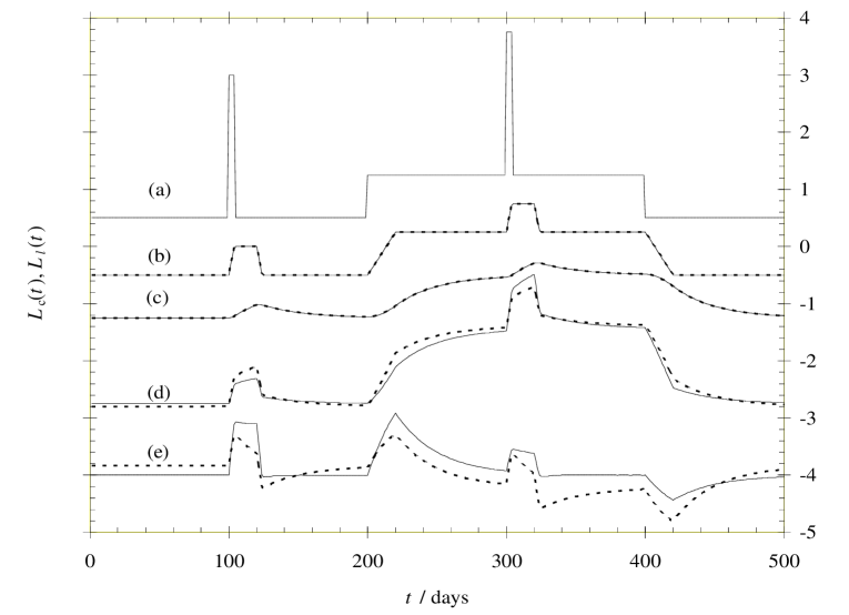
Figure F.1: Comparison of the linear approximation to the actual responses of simple shell-like systems with local delays. Line a is the input continuum that was assumed, which has a luminosity of 0.5 in arbitrary units, the “low state,” followed by a luminosity of 1.25 units, the “high state,” which lasts for 200 days. Superimposed upon the low and high states are delta-function-like spikes of area 10 unit-days. The solid lines ${\it b}-{\it e}$ are the output line luminosities for the models described in the text (§ F.4) offset respectively by -1, -1.75, -3, and -5 luminosity units while the dotted lines are approximations of the outputs obtained from linearized response functions. Though the linearized responses do a reasonable job of matching the actual responses for most of the models shown here, they fail to exhibit the differences between weak and strong (time-integrated) excitation. This is particularly evident for the model shown in solid line e.

These effects can be seen more clearly by considering a simple shell-like system in which the light crossing time is slightly shorter than the cloud equilibrium time. Specifically, let $f({\bf r},{\bf v})\propto\delta(r-10$ days$\cdot c)$, the asymptotic cloud area function be $A^{\prime}(F_{{\scriptsize\rm c}})=A_{0}(F_{{\scriptsize\rm c}}/F_{0})^{\alpha},\tau_{A}=30$ days, $\epsilon_{\hbox{{\scriptsize\rm A}{\scriptsize\it l}}}$=$0,\epsilon_{l}=1,$ and the normalization of $f$ determined by the condition that the mean covering factor be unity, i.e., $<F_{l}>=<F_{{\scriptsize\rm c}}>$. The ratio of the area equilibrium time to the light crossing time of this system is 3, which is near enough to 1 for neither the fast nor the slow cloud regime (§ F.3) to be applicable. Exact outputs obtained upon application of equations (F.4)-(F.5) for various values of $\alpha$ of this system are displayed as solid lines $b,~{}d$, and $e$ of Figure F.1, while the input continuum that was assumed is shown as the solid line a. This input is a “low state” followed by “high state” that lasts for 200 days. Superimposed upon the low and high states are delta-function-like spikes of area 10 luminosity-unit-days, the responses of which can give a crude indication of a spatial response function of the system. The outputs from the linearized response functions are shown as dotted lines. Ideally the optimal linearized response functions would have been obtained from a fitting scheme that minimized the discrepancy between the exact outputs. However, in this work they were obtained simply from equation (H.4), equations (F.6)-(F.8), and finally equation (H.13), which was derived for sinusoidal-like inputs but which results in surprisingly good fits for the input here as well.

For the nonreactive $\alpha=0$ case shown in solid line $b$, the gain of the output line luminosity is unity, and the linearized response function of the system is just the spatial response function, which is a step function. Whether in the high or low state, here the amplitude of the response on time scales larger than the spatial time is the same as that of the input. The $\alpha=1$ model is shown in solid line d. For this reactive model the cloud area responds linearly to the local continuum flux. This is shown explicitly in line c, which is the time-dependent area of the clouds on the shell after the spatial delay was removed by artificially setting $f({\bf r},{\bf v})\propto\delta(r)$. Care must be taken in the interpretation of this response, as the actual size of this system is infinitely smaller than the size that the formalism of Blandford & McKee (1982) would yield, which is $\sim 40$ light-days$\sim c\tau_{\max}/2,$ where $\Psi_{F_{l}|F_{{\scriptsize\rm c}}}(\tau>\tau_{\max})\simeq 0.$ It is important to understand that although the cloud areas respond linearly in the $\alpha=1$ model, the output itself is over-responsive compared to linear, with an asymptotic gain of 2 (eq. [F.6]). This asymptotic gain is also approximately the correction factor by which the formalism of Blandford & McKee (1982) could overestimate the cloud number density. (The exact factor is dependent upon the input, as eq. [H.13] indicates, as well as the fitting criteria.) However, by taking into account an asymptotic gain correction factor that is different from unity, the linear response (dotted line ${\it d})$ does a surprisingly good job of fitting the actual response (solid line ${\it d})$ of the system, especially given that the input continuum luminosity function varies by a factor 7.5.

Nonlinear response is more apparent in the “under-responsive” $\alpha=-1$ model shown in solid line e. Here the cloud area response is given by a nonlinear input-modified system (eq. [H.8]). A key difference between the models shown in solid lines ${\it d}$ and ${\it e}$ is that the gain of an individual cloud area is a decreasing function of positive frequency for the over-responsive model, but is an increasing function for the under-responsive model. Note that because the areas of the spikes are small, the actual responses to the first spike are similar in both cases. The spatial response function (solid line $b)$ does a crude job of describing both models. However, low frequency or high (time-integrated) energy excitation exposes the latent nonlinearities of these systems. For instance, the over-responsive system (solid line $d)$ responds slightly higher to the spike in the high state than the spike in the low state, while the linearized response function predicts a response that was the same strength for both spikes. This aspect of behavior is due to a nonlinear asymptotic gain. Even if it were accounted for, the shapes given by the linearized response function would still not perfectly match the exact ones. For instance, the linearized output for the over-responsive system responds too rapidly to the beginning of the high state. If its linearized response function were adjusted to yield a slower response, the linearized output would then respond too slowly to the beginning of the spike in the low state. Ultimately this is due to the area factor and hence the area equilibrium time playing a less important role in the response to the first spike of short duration (when the area is relatively constant) than in response to the energetic high state of long duration (when the area increases significantly). These types of problems are particularly evident for the highly nonlinear under-responsive case. Because the amplitude of the asymptotic gain of the area is only 1, the response to both low energy spikes is square-like. However, the high state is energetic and long enough to permit the areas to respond and the asymptotic gain of zero nearly to be attained, which results in triangle-like responses. The linearized response function incorrectly gives triangle-like features in the responses to the spikes.

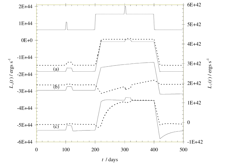
Figure F.2: Effect of the pressure equilibrium time upon the “line-specific” response. The top line (left axis) is the input continuum luminosity assumed. The exact Ly$\alpha~{}($solid lines) and C IV (dotted lines) output luminosities (left axis) are also shown for three extremely simple $s=1$ models similar to those shown in Fig. F.1. To emphasize the effect of just the cloud pressures and pressure ionization parameters being locally delayed, the cloud areas were artificially forced to yield a constant geometrical covering factor of unity (neglecting absorption) and the cloud column densities were artificially forced constant at $10^{22}$ cm^-2. The initial column density to pressure ionization parameter ratios assumed were $1.2\times 10^{22}$ cm^-2. The line luminosities for models ${\it b}$ and c are offset respectively by $-10^{42}$ and $-3\times 10^{42}$ ergs s^-1. The pressure-equilibrium times $\tau_{P_{l}}$ assumed in models ${\it a},{\it b}$, and c were respectively 1.1, 500, and 30 days. For pressure-stratified clouds, this respectively corresponds to wave propagation speeds of $\sim c_{{\scriptsize\rm s}}~{}($pressure-limited evaporation$),\sim 2\times 10^{-3}c_{{\scriptsize\rm s}}~{}($thermal evaporation), and $\sim 4\times 10^{-2}c_{{\scriptsize\rm s}}~{}($intermediate evaporation), where $c_{{\scriptsize\rm s}}$ is the sound speed. The photoionization code that was used is XSTAR (see, e.g., Kallman 1995). The spectrum that was assumed is shown in Fig. F.3.

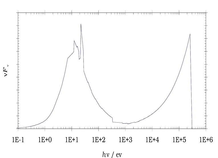
Figure F.3: The spectrum that was assumed for the models shown in Fig. F.2. It is identical to that used in Krolik et al. (1991). Note that the $y$-axis is plotted in linear (as opposed to logarithmic) coordinates.

For the models shown in Figure F.1, all the cloud property gain terms in equation (F.6) except that of the area are zero. However, for calculations of relative line strengths, the ionization parameter gain term in equation (F.6) frequently determines the key distinguishing response characteristics. This is illustrated by the models shown in Figure F.2, where the response as a function of the pressure equilibrium time scale is shown for three models nearly identical to those used in Figure F.1. However, for these cases, $P\propto F^{s/2}_{{\scriptsize\rm c}}$, the cloud areas and column densities are forced to be constant, and the spike strengths are reduced. For model a, the pressure equilibrium time is 1.1 days, which is approximately the mean inverse Strömgren sound crossing time for these clouds. This is short enough (compared to the spatial time of 10 days) for the fast cloud regime to be valid. Thus, in this case, a single (rather than double) integration in lag would have sufficed for calculating $L_{l}(t)$. For model ${\it b}$, the pressure equilibrium time is 500 days, which is closer to the thermal evaporation time scale (Table F.1) of $\sim 2\times 10^{3}$ days. In the limit in which the pressure equilibrium time scale becomes infinite, model ${\it b}$ is identical to a nonreactive $s=0$ model, which also would not require the computationally expensive double integration. Finally, for model c the equilibrium time scale is 30 days. This intermediate equilibrium time might be applicable for cloud models in which the evaporation rate is a strong function of the mean ionization state (see also Taylor 1994). Because the column density to pressure ionization parameter ratio $(1.2\times 10^{22}$ cm${}^{-2})$ was selected to place the model near the “C IV—limited” state in which the C IV gain is $\sim-1,$ the C IV line responds very weakly to the initial spike. However, it responds strongly on the pressure equilibrium time scale to the beginning of the extended high state, during which time the pressure regulation mechanism readjusts the ionization parameter partially back toward its lower initial equilibrium value. In contrast, at the ending of the high state, the C IV line drops on the shorter spatial time scale because of the higher pressures (and lower ionization parameters) of the clouds. This example illustrates one of several ways in which the mean response time of a system can be dependent upon the recent mean continuum luminosity.

The above examples clearly illustrate how the global linearized response function can have structure not due to the spatial response function. However, nonlinear effects can even mask the spatial information. For example, if the ratio of the local continuum flux to the product of the mean pressure and column density of the clouds becomes high enough, the emission of certain lines could be “recombination-limited,” which makes $\tilde{\hat{\Psi}}_{\epsilon_{l}|F_{{\scriptsize\rm c}}}(\infty)\sim-1$ in equation (F.6). This occurs during the high state with Ly$\alpha$ for model ${\it b~{}}($solid line Fig. F.2). Therefore, as the model shown in the solid line c of Figure F.1 also illustrates, the response times give, under the assumption of spherical symmetry, only upper limits to the characteristic size.

The above examples also help illustrate how local delays can affect the cross-correlation function. Consider a simple $\eta(A|F_{{\scriptsize\rm c}})>0$ model, such as that shown in solid line ${\it d}$ of Figure F.1. For a weak enough high frequency square wave input occurring above a steady input background, the output would be a capped triangle wave, which is symmetric about its peak with respect to lag. The cross-correlation function that one would obtain from such data would be shifted of approximately a day, yet also be symmetric about the characteristic lag. This is because the data from the beginning, or growing phase of the pulse, which alone would produce a cross-correlation function with a positive slope, is compensated by the ending or falling phase of the response pulse.

Consider, however, the case wherein the input is a moderate-intensity, low frequency square wave. Because of local delays, the response would be higher near the end of the pulse, as in solid line ${\it d}$ of Figure F.1a. Since the cross-correlation function is an amplitude-biased function, the resulting cross-correlation function would be biased from the data in the falling phase. Unlike the previous case, this would result in a negatively sloped component to the cross-correlation function, which is quite common (e.g., Sparke 1993).

Note that local delays only give the cross correlation function asymmetry about their peak above what one would obtain from the global linearized response function alone. This is because the cross-correlation function is the convolution of the response function and the symmetric, input auto-correlation function. For this reason, assessing the importance of asymmetric cross-correlation functions in determining the characteristics of the local delays of interest here would probably require knowledge of the best-fitting linear response function.

Note that this function would be biased somewhat by the low energy (more symmetric) pulses. Therefore, the asymmetry of the “simulated cross-correlation function” that one would obtain from the output of this response function would not be as great as the one obtained from actual variability data. Thus, the difference between the simulated and actual cross-correlation functions can be asymmetric if local delays are important. This permits a simple way of testing for local delays.

F.5 Summary and Conclusions

In this appendix it has been argued that for some reactive cloud models the fast cloud assumption is invalid. In such cases a tight correspondence between the positional distribution of matter and the global linearized line flux response function simply does not exist. This is because the continuum luminosity at a given time in history affects not only the clouds on a spherical shell, but also the clouds inside such a shell. In general, the response which results is not only nonlinear, but also inseparable, requiring more than one integration over lag to determine the output flux at a specified time. However, in some cases the time-dependence of the line fluxes can be described using linearized response functions $\Psi_{F_{l}|F_{{\scriptsize\rm c}}}$. These response functions have structure at intermediate lags due to the finite size of the line-emitting region and at lags greater than these due to the finite equilibrium times of the line-emitting material itself. For small enough perturbations the physical cloud properties can be relatively static and a linear response function can work quite well at describing the responses. However, when the input continuum variations become extreme enough, such response functions can fail. Because of nonlinear asymptotic response, the integral of a linearized response function of an observable differs from the time average of the observable by a correction factor of the asymptotic gain. Ignoring nonlinear effects can lead to incorrect measurements of the physical properties of the system, such as sizes that are too large.

One of the most fundamental assumptions that has been made in previous analysis of variability data has been the fast cloud assumption. With this assumption now in question, this data should be examined again with models that do not require it.

Appendix G The Line Flux of a Cloud When the Equilibrium and Crossing Times are Comparable

In standard references such as Blandford & McKee (1982), the time-dependent line profile is presented as an integral over the cloud phase space of distribution function and emission flux. The line emission from these clouds is implicitly assumed to be independent of the direction of their velocity vectors. As a result, in order for these models to generate the line shifts and asymmetries which are observed, the clouds must generally flow outwards or inwards. Models with such radial flow can, however, have serious problems, such as very low accretion efficiencies (see, e.g., Kallman et al. 1993).

Before one invests substantial effort to concoct models which address these problems, it may be worthwhile to ${\rm re}$-analyze the original, highly intuitive conclusion that line emission from clouds is independent of the direction of their velocity vectors. In fact, a careful examination reveals that, because of our extreme ignorance of what the clouds in AGNs are, there are several theoretically permissible reasons that clouds could (at least in principle) have line emission dependent upon their velocity direction. Each of these reasons is the result of an uncertainty in a corresponding assumption made either explicitly or implicitly in Blandford & McKee (1982) and similar works. By examining each of these assumptions in detail, we clearly outline the boundary of parameter space in which the velocity-direction-independent emission result must lie. Moreover, by looking just outside these boundaries we could obtain a model which does not suffer as severely from the types of problems plaguing current AGN models.

In this appendix we will focus on just one of the potentially invalid assumptions made in previous works, i.e. that the cloud equilibrium times are negligible compared to the cloud crossing times. As shown in Table F.1, this assumption is invalid for some models. For these models, the cloud properties have an additional explicit dependence upon the prior continuum fluxes $F_{{\scriptsize\rm c}}{\hbox{\bf(}}t-\tau,{\bf r}(t-\tau){\hbox{\bf)}}$ and hence the orbital trajectories of the clouds, which is a different function for each cloud. This would complicate modeling efforts, which would entail integrating over the orbital trajectories of the clouds. It could also make the much simpler approach taken by Blandford in McKee (1982) invalid. However, we shall find that in certain cases the cloud luminosity function can be described merely by giving the properties of the cloud an additional velocity-direction dependence.

But let us first obtain the exact solution to this problem. Ignoring absorption, the (nonlinear) line flux as a function of time for a cloud is given by application of equation (F.3) to each of the cloud parameters in equation (F.4). Thus, the continuum-subtracted, time-dependent line profile of the “global” system observed from ${\bf D}$ is

$$F_{l}(t,v_{D})=\sum^{N}_{i=1}F^{\hbox{{\scriptsize\rm orb}}}_{li}(t)\delta(v_{D}+{\bf v}_{i}\cdot\hat{{\bf D}}),$$ (G.1)

where $N$ is the number of clouds and $F^{\hbox{{\scriptsize\rm orb}}}_{li}$ is the flux in line $l$ from cloud i computed from the forms of equations (F.3)-(F.4) appropriate for the model to be tested. Neglecting absorption and non-Doppler line broadening, equation (G.1) gives the exact time-dependent line profile for clouds with arbitrary motions. However, because the suspected number of clouds in AGN is high (e.g., Laor et al. $1994;cf$, e.g., Peterson 1994), using it could prove computationally expensive.

Noting the exponential factor in equation (F.3), integration over the history of local continuum exposure required for determining the cloud properties at a given time need only be carried out to a small factor (e.g., $\sim 4)$ of the relevant equilibrium time. Therefore, if each cloud property relevant to emission has an equilibrium time scale that is appreciably less than the emission region crossing time, the radius will not change drastically over the relevant history interval, and the continuum flux function can be approximated by its Taylor expansion. This yields a first order correction to the continuum flux function that is proportional to the radial velocity. Similar expansions permit estimation of the line flux observed from an individual cloud and the line shifts that equation (G.1) implies.

However, if $N$ is independent of the continuum flux and is large enough that line broadening produces a smooth line profile, a more accurate method for obtaining the individual cloud line flux that partially accounts for higher order terms can be obtained simply by taking the statistical average of the function, which is

$$F^{{\scriptsize\rm cl}}_{l}(t,{\bf r},{\bf v};{\bf D})=\lim_{\delta r,\delta v\rightarrow 0;N\rightarrow\infty}{1\over f({\bf r},{\bf v})\delta^{3}r\delta^{3}v}\times\qquad\qquad\qquad\qquad\qquad\qquad\qquad$$

$$\sum^{N}_{i=1}\int^{{\bf r}+\delta{\bf r},{\bf v}+\delta{\bf v}}_{{\bf r},{\bf v}}d^{3}r^{\prime}d^{3}v^{\prime}\delta{\hbox{\bf(}}{\bf r}^{\prime}-{\bf r}_{i}(t){\hbox{\bf)}}\delta{\hbox{\bf(}}{\bf v}^{\prime}-{\bf v}_{i}(t){\hbox{\bf)}}F^{\hbox{{\scriptsize\rm orb}}}_{li}(t).$$ (G.2)

The dependence of $F^{{\scriptsize\rm cl}}_{l}(t,{\bf r},{\bf v};{\bf D})$ upon time is due to the variation of the continuum flux to which the cloud is locally exposed. The dependence upon position is due to traditional model elements such as changes in the mean cloud density as a function of average heating. Finally, the dependence upon the velocity vector accounts for the intrinsic dependence as well as that due to the history of heating being important when the equilibrium time scale is not completely negligible compared to the emission region crossing time. Note that for models where the position and velocity variables impose the integrals of motion of a trajectory of a cloud, the above condition that the equilibrium times are small compared to the crossing times is unnecessary and the flux is an exact function of only the time, position, and velocity variables.

In this case, an analog of equation (G.2) can be used to replace the knowledge of the individual cloud trajectories with the time-independent phase space distribution function $f({\bf r},{\bf v})$. Though this function, when combined with equation (G.2), permits equation (F.5) to be used to obtain an approximation of the time-dependent line profile, it offers little advantage over using just equation (G.1) because it still entails explicit time-dependent orbital modeling.

However, in the linear regime (eqs. [F.7]-[F.8]), only the time-average of equation (G.2) is required to obtain the time-dependent line profile. Once this (velocity-dependence) has been computed for a model, the linear approximations to the observable characteristics can be obtained from equation (F.8) for various continuum light curves without explicit time-dependent orbital modeling. Therefore, in the linear regime, the orbital history of the cloud line emission flux can be approximated as a simple function of the direction and magnitude of the cloud velocity vector $\hat{{\bf v}}$.

Appendix H Response of Nonlinear Systems in the Linear Regime

In Blandford & McKee (1982), linear systems were analyzed in the linear regime. In this appendix a formalism is developed for analyzing nonlinear systems in the linear regime. Though the solution to this problem is a straightforward and probably necessary prerequisite for any comprehensive understanding of variability in AGN, it was not correctly obtained or applied in other works regarding AGN variability. We shall find that within the linear regime the analysis in Blandford & McKee (1982) is inadequate for general nonlinear systems.

Let us consider the generic system described in § F.3.1. Using the notation of § F.3.1 for $y(t),y^{\prime}(x),x(t)$, and $t$, there is no reason that $\delta y^{\prime}(x)\propto\delta x$ should generally hold, and one may be forced to employ a fully nonlinear analysis method to accurately describe the system. However, let us assume here that the variations in $x$ are sufficiently smaller than its mean, in which case, provided $y^{\prime}(x)$ is a smooth function, it can be approximated with

$$y^{\prime}=<y>\left[1+\eta(y|x)\left({x\over<x>}-1\right)\right]\pm\sigma_{y},$$ (H.1)

where the dimensionless, “asymptotic gain” $\eta$ of changes in $y$ for small and slow changes in $x$ is defined by

$$\eta(y|x)\equiv\lim_{\delta x,\dot{x}\rightarrow 0}{\delta y/y\over\delta x/x}={<x>\over<y>}{\partial y^{\prime}\over\partial x}|_{x=<x>},$$ (H.2)

where $\sigma_{y}$ is the error due to nonzero second order derivatives in $y^{\prime}$. The asymptotic gain has elsewhere been termed the “responsivity” (Krolik et al. 1991; Goad, O’Brien, & Gondhalekar 1993). Here it is an operator to distinguish between the various gains with the different “output” and “input” functions that will be required, though note that it is independent of the normalizations of these functions.

Let us extend the definition of gain by allowing a dependence upon the type of input signal. Consider a time-dependent local ionizing continuum flux or a Fourier component of it such as $x(t)-x_{0}=x_{1}\cos(\omega t)$. A dimensionless frequency-dependent gain or transfer function $\tilde{\hat{\Psi}}$ of $y({\it t})$ with respect to $x(t)$ can then be defined as

$$\tilde{\hat{\Psi}}_{y|x}(\omega)\equiv\lim_{\delta x\rightarrow 0}{\delta y/y\over\delta x/x}|_{\ddot{x}/x_{1}=-\omega^{2}}.$$ (H.3)

Letting $\tilde{y}(\omega)$ denote the Fourier transform of $y({\it t})$, etc., gives

$$\tilde{\hat{\Psi}}_{y|x}(\omega)={<x>\over<y>}{\partial\tilde{y}(\omega)\over\partial\tilde{x}(\omega)}$$ (H.4)

and an analog of the Fourier transform of equation (H.1) for a frequency-dependent gain,

$$\tilde{y}(\omega)\simeq<y>\left[\delta(\omega)+\tilde{\hat{\Psi}}_{y|x}(\omega)\left({\tilde{x}(\omega)\over<x>}-\delta(\omega)\right)\right].$$ (H.5)

With this notation, $|\tilde{\hat{\Psi}}_{y|x}(\omega)|$ is the dimensionless ratio of the amplitudes of variations of $y$ to $x$, while -Im$[\ln{\hbox{\bf(}}\tilde{\hat{\Psi}}_{y|x}(\omega){\hbox{\bf)}}]/\omega$ is the delay in response. Similarly, the asymptotic gain is Re$[\tilde{\hat{\Psi}}_{y|x}(0)]$, while the “instantaneous component of the gain” is Re$[\tilde{\hat{\Psi}}_{y|x}(\infty)]$.

Equation (H.5) yields in the time domain

$$y(t)=<y>\left[1+\int d\tau\left({x(t-\tau)\over<x>}-1\right)\hat{\Psi}_{y|x}(\tau)\right]\pm\sigma_{y},$$ (H.6)

where we define the inverse Fourier transform of the gain of the output $y({\it t})$ with respect to the input $x(t)$ as the normalized linearized response function, which is

$$\Psi_{y|x}(\tau)\equiv{<y>\over<x>}\hat{\Psi}_{y|x}(\tau).$$ (H.7)

Here the lack of a caret denotes that the normalized response function has scaling other than that given to it by the inverse Fourier transform. Note that the integral of the linearized response function is just the asymptotic gain, which is only unity for actual linear systems.

Linearization is not always advantageous. In some cases, including those obeying equation (F.1), the exact solution can easily be obtained from

$$y(t)=\int d\tau y^{\prime}{\hbox{\bf(}}x(t-\tau){\hbox{\bf)}}\Psi_{y|y^{\prime}}(\tau),$$ (H.8)

where

$$\Psi_{y|y^{\prime}}(\tau)=\hat{\Psi}_{y|y^{\prime}}(\tau)=\hat{\Psi}_{y|x}(\tau)/\eta(y|x)$$ (H.9)

is the response function of an “input-modified” system.

However, linearization can be quite useful, in some cases it allows complex systems to be accurately described by a single equivalent response function, which can drastically reduce the simulation time. Such is the case wherein one is interested in obtaining an observable quantity of a system with many clouds, wherein the convolution of $y$ with a spatial linear response function must be evaluated. For instance, consider a hypothetical system wherein a physical cloud property $z^{\prime}(y)\propto y^{\eta(z|y)}$ lags property $y$ on a time scale $\omega^{-1}_{z}$, while property $y^{\prime}(x)\propto x^{\eta(y|x)}$ has a “direct” lag of $\omega^{-1}_{y}$. The exact expression for $z({\it t})$ has two nested integrals over lags. However, upon linearization the transfer function of $z$ for small variations in $x$ is

$$\tilde{\hat{\Psi}}_{z|x}(\omega)={\eta(z|y)\over 1+i\omega/\omega_{z}}{\eta(y|x)\over 1+i\omega/\omega_{y}},$$ (H.10)

or alternatively

$$\hat{\Psi}_{z|x}(\tau)=\Theta(\tau)\eta(z|y)\eta(y|x)\omega_{z}\omega_{y}\left({e^{-\omega_{z}\tau}\over\omega_{y}-\omega_{z}}+{e^{-\omega_{y}\tau}\over\omega_{z}-\omega_{y}}\right)\qquad\{\omega_{y}\neq\omega_{z}\}\qquad\qquad$$

$$=\Theta(\tau)\eta(z|y)\eta(y|x)\omega^{2}_{z}\tau e^{-\omega_{z}\tau}~{}~{}\qquad\qquad\qquad\qquad\{\omega_{y}=\omega_{z}\},$$ (H.11)

which when applied (in eq. [H.6]) requires only a single integral over lag. For future reference, note that when $\omega_{z}\gg\omega_{y}$ or $\omega_{z}\ll\omega_{y}$, the two gain factors are “separable” from one another, i.e. for a restricted range of excitation frequencies one of the gain factors can be treated as a constant.

In this section it has been shown (eq. [H.9]) that there is a “correction factor” of $\eta(y|x)$ in the expression for the “gain-corrected response function.” Previous works (e.g., Blandford & McKee 1982) assumed that the systems themselves are linear, which is equivalent to assuming correction factors of unity. Some of the problems with making this assumption are pointed out in Goad, O’Brien, & Gondhalekar (1993) as well as § F.4 of this work. Note that the correction factors differ from unity in equation (H.2) in nonlinear systems even if the perturbations are arbitrarily small and equation (H.6) accurately describes the system.

Partially accounting for even higher order corrections due to nonlinearity is also possible within the linear regime and, in fact, is important for accurate interpretation of fits of linear models to nonlinear systems. If the variations are not infinitesimal, the above equations do not necessarily yield the “optimal” fit that would have obtained using real variability data. For instance, consider the case wherein $y^{\prime}=y_{0}(x/x_{0})^{\alpha}$. The better-fitting optimal average for a sinusoidal-like input is the first Fourier coefficient of $y^{\prime}$,

$$<y>={1\over 2\pi}\int^{2\pi}_{0}d(\omega t)y^{\prime}{\hbox{\bf(}}x_{0}+x_{1}\cos(\omega t){\hbox{\bf)}}\neq y^{\prime}(<x>).$$ (H.12)

Similarly, the observable asymptotic gain is approximately

$$\eta(y|x)={1\over\pi}\int^{2\pi}_{0}d(\omega t)\cos(\omega t){y^{\prime}{\hbox{\bf(}}x_{0}+x_{1}\cos(\omega t){\hbox{\bf)}}\over<y>}\neq\alpha,$$ (H.13)

where the inequalities can be removed only for the $x_{1}\ll x_{0}$ case.

Appendix I Velocity Deconvolution Techniques

I.1 Assumptions and Background

As discussed in Chapter 2, the response functions shown in Chapter 4 were made under the questionable assumption that the wind size equilibrium times are small compared to the light crossing times. As shown in Appendix F, without this assumption the response is more complex and longer than what would be inferred from the spatial distribution of clouds alone. This is unfortunate, as the original motivation behind reverberation mapping was to constrain this spatial distribution of clouds.

In this appendix, I show that under certain conditions the spatial distribution of clouds can nevertheless be measured even if the clouds have response times comparable to the light crossing times. Thus, even if the cloud reaction times are of the order of the cloud crossing times, the original goal of reverberation mapping may be obtainable after all, at least for certain classes of models.

I also show that the response functions of properties of individual clouds, i.e., the “cloud response functions,” can be measured. Knowledge of these cloud response functions would impose very specific and severe constraints upon the confinement mechanisms that are invoked in various cloud models and help resolve the question of what the clouds are if the cloud concept is indeed valid.

I.2 Separating the Spatial and Cloud Transfer Functions

In this section, we first define a mathematical transformation that can be applied to line profiles. In § I.2.2, we use this transformation to derive expressions for the individual cloud response functions. We find that for certain values of the characteristic cloud equilibrium time scales, the qualitative response features can be obtained without explicit use of both the cloud and spatial response functions. In § I.2.3 the precise conditions for this simplification are calculated.

There are a wide variety of cloud models that have been proposed. The results of this appendix, however, are valid only for a small subset of them. In particular, in the remainder of this appendix, we assume that the clouds are in orbital motions inside a centrally symmetric gravitational field; the results of this appendix do not generally apply to models violating this assumption.

I.2.1 Obtaining the Line Intensity

The primary observable of an AGN is its spectrum. One of the simplest ways of analyzing a spectrum is to break it up into an underlying continuum and several line profiles that are functions of an equivalent line-of-sight velocity $v_{{\scriptsize\rm D}}$. These profiles can then be compared to theoretical ones to gauge the viability of a model, or, more quantitatively, measure the goodness of a model.

Unfortunately, the line profile is somewhat inadequate for our purpose here. In this appendix we find that in order to determine some of the key response characteristics of the flux of a line, it is useful to work with a variable that is more closely coupled to the radius than is $v_{{\scriptsize\rm D}}$.

It is well known that the integral of the spectrum is the bolometric luminosity or flux. For this reason, we can consider the spectrum to be the “wavelength representation” of the bolometric luminosity. Similarly, we can consider the line profiles $F_{l}(t,v_{{\scriptsize\rm D}})$ as a function of time $t$ to be a representation of the continuum-subtracted flux in $v_{{\scriptsize\rm D}}$-space. The response functions are yet other representations of the flux.

In this appendix we employ a new representation of the line flux. Consider the integral transform

$$F_{l}(t,v_{{\scriptsize\rm D}})=\int d\sigma I_{l}(t,\sigma)\phi_{l}(\sigma,v_{{\scriptsize\rm D}}),$$ (I.1)

where $F_{l}$ is the continuum-subtracted line flux, $\phi_{l}(\sigma,v_{{\scriptsize\rm D}})$ is the kernel of the integral transform, and $I_{l}$ is a new function herein termed the “line intensity,” which, incidentally, has no relation to the variable commonly used in radiative transfer calculations. The above equation maps the representation of the line flux in $\sigma$-space $I_{l}(\sigma,v_{{\scriptsize\rm D}})$ to the representation of the line flux in $v_{{\scriptsize\rm D}}$-space. Were $\phi_{l}(\sigma,v_{{\scriptsize\rm D}})$ constrained to form an orthogonal and complete basis, the mappings between $I_{l}$ and $F_{l}$ would be unique. However, for generality, $\phi_{l}(\sigma,v_{{\scriptsize\rm D}})$ is permitted to be overcomplete here. This does not pose serious problems because only discrete forms of $I_{l}$ are applied to equation (I.1). Thus, the resolution in $\sigma$-space can always be limited such that the mapping from $F_{l}$ to $I_{l}$ is undercomplete and well-constrained. In this respect, the only condition that we initially impose upon $\phi_{l}(\sigma,v_{{\scriptsize\rm D}})$ is that its integral with respect to $v_{{\scriptsize\rm D}}$ be unity.

What particular advantage does the $\sigma$-representation offer over the $v_{{\scriptsize\rm D}}$-representation? Let us assume that a unique mapping between distance from the black hole ${\it r}$ and $\sigma$ exists with the function $r(\sigma)$. This permits the radial integration in the time-dependent line profile (eq. [F.5]) to be removed. Doing this yields

$$I_{l}(t,\sigma)=|{\partial r\over\partial\sigma}|r^{2}\int d\Omega_{r}{d^{3}vf({\bf r},{\bf v})\delta(v_{{\scriptsize\rm D}}+{\bf v}\cdot\hat{{\bf D}})\over\phi_{l}(\sigma,v_{{\scriptsize\rm D}})}F^{{\scriptsize\rm cl}}_{l}(t,{\bf r},{\bf v},{\bf D}),$$ (I.2)

where the dependence of $r$ upon $\sigma$ is implicit, $\Omega_{r}$ is the solid angle of the spatial vector ${\bf r}$ from the black hole, $F^{{\scriptsize\rm cl}}_{l}(t,{\bf r},{\bf v},{\bf D})$ is the flux from a cloud at ${\bf r}$ with velocity ${\bf v}$ in line $l$ observable from ${\bf D}$, and $f$ is the probability distribution of clouds in phase space. The above expression is an integral over spatial angle, velocity, and (in its most general form) the history of the local continuum flux via $F^{{\scriptsize\rm cl}}_{l}$. The kernel of the transform $\phi_{l}(\sigma,v_{{\scriptsize\rm D}})$ can be defined to be the average of the local line profile composed of clouds on the shell with radius $r(\sigma)$. With this definition, the fraction in the integral of equation (I.2) becomes equal to the mean density of clouds on this shell. Thus, equation (I.2) can be viewed simply as a summation of the line flux received from clouds on the shell of radius $r(\sigma)$. In fact, $\sigma$ can be interpreted as a velocity dispersion parameter while the local profile $\phi_{l}(\sigma,v_{{\scriptsize\rm D}})$ can be defined such that $3\sigma^{2}\sim~{}<v^{2}>~{}\simeq GM_{{\scriptsize\rm h}}/{\it r}$, where $M_{{\scriptsize\rm h}}$ is the black hole mass and $G$ is the gravitational constant.

Note that the clouds contributing toward the line intensity at a specific velocity dispersion $\sigma$ are restricted to lie on a shell that is a fixed distance from the black hole. This is in contrast with the line profile at a specific equivalent line-of-sight velocity $v_{{\scriptsize\rm D}}$, which is an integral over all radii. In the next subsection, we see how this feature can permit measurement within the context of a model of the cloud response functions from the intensity light curve.

However, let us first review two key prerequisites for applying equation (I.1) to measure (constrain) the line intensities $I_{l}$ from a given spectrum:

1. knowledge of $r(\sigma)$ and

2. knowledge of the local line profiles $\phi_{l}(\sigma,v_{{\scriptsize\rm D}})$.

In Appendix J, it is shown how both $r(\sigma)$ and $\phi_{l}(\sigma,v_{{\scriptsize\rm D}})$ can be obtained for certain simple orbital models. The methods discussed in Appendix J are inapplicable for non-orbital models. Therefore, for non-orbital models, reliable measurements of $I_{l}$ from a spectrum could be difficult if not impossible. For the orbital models considered in this appendix, however, accurate measurement of $I_{l}$ from a given spectrum should be achievable at several different points in dispersion space. Thus, if we restrict ourselves to orbital cloud models, the “intensity light curves” can be measured from time-resolved spectra, provided that they are available. Incidentally, this particular theoretical feature of orbital models is definitely not a reason for invoking them. It merely permits a particular type of analysis to be performed that would otherwise be much more difficult.

I.2.2 Obtaining the Cloud Transfer Functions

This appendix concerns response functions of several different time-dependent quantities. For this reason, we employ a notation that explicitly denotes what is the specific “input” and “output” of a response function. In particular, let us define the “linearized response function” of an arbitrary output variable $y$ as a function of lag $\tau$ to be $\hat{\Psi}_{y|x}(\tau)$ when the input variable is ${\it x}$ and the variations are small enough about their means that the system can be considered to be linear (see Appendix H). With this notation, the dimensionless Fourier transform of the linearized response function of the line profile at a given line-of-sight velocity $v_{{\scriptsize\rm D}}$ with respect to the observed continuum flux $F_{{\scriptsize\rm c}}$ is

$$\tilde{\hat{\Psi}}_{F_{l}|F_{{\scriptsize\rm c}}}(\omega,v_{{\scriptsize\rm D}}).$$ (I.3)

An expression for this quantity, which is also called the two-dimensional transfer function or “global gain” of the line profile, is provided by equation (F.7). It contains an integral over all radii. For this reason, it has nontrivial structure (is not flat in $\log-\log$ coordinates) over a large range of lags, even with $v_{{\scriptsize\rm D}}$ held constant.

Let us now calculate the transfer function of the line intensity with respect to the continuum flux. Applying the formalism of Appendix H yields

$$\tilde{\hat{\Psi}}_{I_{l}|F_{{\scriptsize\rm c}}}(\omega,\sigma)=|{\partial r\over\partial\sigma}|r^{2}\int d\Omega_{r}d^{3}v{<F^{{\scriptsize\rm cl}}_{l}(t,{\bf r},{\bf v},{\bf D})>_{t}\over<I_{l}(t,\sigma)>_{t}}\times\qquad\qquad\qquad\qquad\qquad\qquad\qquad\qquad$$

$$f({\bf r},{\bf v})\tilde{\hat{\Psi}}_{F^{{\scriptsize\rm cl}}_{l}|F_{{\scriptsize\rm c}}}(\omega)e^{-i\omega(\hat{{\bf r}}-\hat{{\bf D}})\cdot{\bf r}/c},$$ (I.4)

where the dependence of $r$ upon $\sigma$ is again implicit. The above equation states that gain of the intensity at a given excitation frequency and dispersion $\sigma$ is proportional to the time-averaged, angle-dependent line flux of the clouds at $r(\sigma)$; the local line flux gain of such clouds; and a factor that is a strong function of the angle of the position vector of the clouds. Once evaluated, the expression provides an approximation in the linear regime of $I_{l}(t,\sigma)$ given $F_{{\scriptsize\rm c}}(t)$. For reasons discussed in Appendix F, the expression is unique for a given model and mean continuum flux.

While equation (I.4) appears complex, it is actually simple for several models. Many plausible models, for instance, have a time-averaged cloud line flux $F^{{\scriptsize\rm cl}}_{l}$ that is a function of $\hat{{\bf r}}\cdot\hat{{\bf s}}$. Fortunately, this alone does not result in the gain of the cloud line flux having a similar dependence. This is because the gain of the cloud line flux is determined primarily from the mean of the local continuum flux, which is a function only of $r~{}($not $\hat{{\bf r}})$ for many simple yet useful models; the angle-dependent beaming anisotropy factor simply regulates what fraction of the nonlinear flux of a cloud located at ${\bf r}$ is directed towards the observer. On the other hand, some models produce line shifts and asymmetries due to aspherical distribution functions (like those for bulk radial outflow) or with $\hat{{\bf v}}$-dependent cloud pressures (like the one described in Appendix L). At any rate, for the former class of models in which the cloud gain is independent of $\hat{{\bf r}}$ and ${\bf v}$, we can make a neat simplification to equation (I.4). The gain factor can be moved outside the spatial solid angle and velocity integrals in equation (I.4). It can then be written as

$$\tilde{\hat{\Psi}}_{F^{{\scriptsize\rm cl}}_{l}|F_{{\scriptsize\rm c}}}(\omega)={\tilde{\hat{\Psi}}_{I_{l}|F_{{\scriptsize\rm c}}}(\omega,\sigma)\over\tilde{\hat{\Psi}}_{I^{{\scriptsize\rm sp}}_{l}|F_{{\scriptsize\rm c}}}(\omega,\sigma)},$$ (I.5)

where we define $I^{{\scriptsize\rm sp}}_{l}$ to be the “spatial intensity” of the instantaneous component of the cloud responses, i.e., $I_{l}$ if each cloud were to respond linearly with $\hat{\Psi}_{F^{{\scriptsize\rm cl}}_{l}|F_{{\scriptsize\rm c}}}(\tau)$ simply $\delta(\tau)$ for all clouds. As is made clear shortly, the spatial intensity contains the geometrical information about a line’s emission in a model.

If $\tilde{\hat{\Psi}}_{I^{{\scriptsize\rm sp}}_{l}|F_{{\scriptsize\rm c}}}$ could be restricted (computed) to some extent theoretically, the above equation would relate the unique and potentially observable intensity gain to the mean of the linearized transfer functions of clouds on the shell with radius $r(\sigma)$. However, for simple spherical models each of these clouds on this shell responds identically; the response function of the shell is the same as that of each cloud on the shell. Thus, under the above conditions, equation (I.5) can permit measurement of the linearized transfer and response functions of an individual cloud. More precisely, if we account for the finite resolution in velocity dispersion space to which $I_{l}$ has been fit (or deconvolved) via equation (I.1) and the systematic errors in the knowledge of the local line profiles, equation (I.5) permits measurement of the individual cloud transfer functions averaged over a non-zero (but potentially small) range in radii. This is fortuitous. Provided firm theoretical constraints can be imposed upon $\tilde{\hat{\Psi}}_{I^{{\scriptsize\rm sp}}_{l}|F_{{\scriptsize\rm c}}}$, the original dilemma demonstrated in Taylor (1996) regarding “contamination” of the observed response functions by the individual cloud response functions may be tractable after all.

Fortunately for us, $\tilde{\hat{\Psi}}_{I^{{\scriptsize\rm sp}}_{l}|F_{{\scriptsize\rm c}}}$ probably has only a mild model dependence. This can be shown by considering a spherically symmetric model without occulting material. Applying $r(\sigma)=r_{0}(\sigma_{0}/\sigma)^{-2}~{}($where $r_{0}\sigma^{2}_{0}\simeq M_{{\scriptsize\rm h}}G/3)$ to equation (I.4) yields the linearized response function $\hat{\Psi}$ of the spatial intensity

$$\hat{\Psi}_{I^{{\scriptsize\rm sp}}_{l}|F_{{\scriptsize\rm c}}}(\tau,\sigma)=\Theta(\tau)\Theta(2\tau^{{\scriptsize\rm sp}}-\tau){1+\epsilon_{\hbox{{\scriptsize\rm A}{\scriptsize\it l}}}(1-\tau/\tau^{{\scriptsize\rm sp}})\over 2\tau^{{\scriptsize\rm sp}}},$$ (I.6)

where $\epsilon_{\hbox{{\scriptsize\rm A}{\scriptsize\it l}}}$ is the beaming factor in line $l~{}($defined such that $\epsilon_{\hbox{{\scriptsize\rm A}{\scriptsize\it l}}}=-1$ implies fully beamed line emission and $\epsilon_{\hbox{{\scriptsize\rm A}{\scriptsize\it l}}}=0$ implies isotropic line emission) and $\tau^{{\scriptsize\rm sp}}$ is the characteristic “spatial lag” defined as $r(\sigma)$/c. Note that, regardless of the precise value of $\epsilon_{\hbox{{\scriptsize\rm A}{\scriptsize\it l}}}$, the above expression for $\hat{\Psi}_{I^{{\scriptsize\rm sp}}_{l}|F_{{\scriptsize\rm c}}}$ does not have nontrivial structure over a large range of lags. Rather, it is a trapezoidal function having structure at a characteristic delay of $\tau^{{\scriptsize\rm sp}}$. Similarly, $\tilde{\hat{\Psi}}_{I^{{\scriptsize\rm sp}}_{l}|F_{{\scriptsize\rm c}}}$ approaches zero at frequencies significantly above the “spatial frequency” defined here by $\omega^{{\scriptsize\rm sp}}\equiv 1/\tau^{{\scriptsize\rm sp}}$ and is unity at all frequencies significantly below the spatial frequency. Note that for models in which absorption is important (such as those with an occulting accretion disk), the near clouds are relatively brighter, in which case the effects of beaming are to some extent masked. For such models the spatial response function would probably be smoother than equation (I.6) and the spatial gain would be even more constrained to have nontrivial structure only near the spatial frequency. Thus even moderate systematic uncertainties of the models under consideration would probably not foil measurement of the individual linearized cloud response functions.

Equation (I.5) tells us that for some models the intensity gain is simply the product of the spatial intensity and cloud gains. This situation is thus similar to that with equation (H.10), which has the following two general characteristics that can be applied here as well:

1. If the line flux from clouds at a given radius responds linearly then the intensity at the corresponding velocity dispersion also responds linearly. This is because the spatial intensity necessarily responds linearly. Conversely, any nonlinearity in the intensity can be ascribed to nonlinear response of clouds at a particular radius bin. An advantage of this from a modeling perspective is that with predictive photoionization codes one could impose relatively tight constraints upon the cloud parameter space as a function of radius. This is in contrast with modeling the gain of the line profile, which at a specific wavelength is a function of clouds spanning a large range in mean continuum flux. On the other hand, a potential drawback of this is that the intensities at some dispersions would be much more nonlinear than those of the associated profiles because of this lack of radial dilution of cloud response. Therefore, measuring the individual cloud intensity transfer functions could prove difficult at certain dispersions. In this case, the individual cloud transfer functions and equation (I.5) have limited utility in model fitting. Fitting of the physical model parameters using (nonlinear) equation (I.2) could still be done to capitalize upon this richness of the intensity representation. However, as discussed in Appendix F regarding the fitting of nonlinear time-dependent profiles, doing this would be relatively expensive computationally.

2. A second characteristic equation (I.5) shares with equation (H.10) is that the qualitative response features of the intensity can be determined by considering the ratios of the characteristic time scales of the spatial and linearized cloud response functions. For instance, when the ratio differs enough from unity, the cloud line flux and spatial intensity gain factors can be “separable” from one another, and one of the two gain factors can be treated as constant. In this case the time-dependent behaviors at a given excitation frequency depend upon only one of the two time scales of the system.

In the next section we see that the concept of separability can be partially extended to the time domain, where it implies simplified relationships between the three linearized response functions. In this case, equation (I.5) and its application in measuring $\tilde{\hat{\Psi}}_{F^{{\scriptsize\rm cl}}_{l}|F_{{\scriptsize\rm c}}}(\omega)$ simplifies dramatically. Let us now turn our attention to the precise conditions necessary for separability to occur.

I.2.3 Conditions for Separability of the Cloud and Spatial Intensity Gains

Physically, the question of interest is, “Given the various properties of a particular AGN line emission model under consideration in which the clouds take some finite time to react to changes in the continuum flux they experience, which components of the profiles would respond in simple ways?” If, for example, the sampling rate of our data set is only high enough to map out the response from clouds contributing to the narrower profile components, will the emission making up the core of the C IV profile come from clouds that can be treated as responding instantaneously, or will the time-dependent responses of these clouds affect what we observed in our data? If the clouds respond fast enough, the time-dependence of their responses could perhaps be ignored in the narrow emission region but not the broad emission region. This subsection addresses such questions quantitatively.

Let us consider the case in which just one time constant $\tau^{{\scriptsize\rm cl}}_{l}=1/\omega^{{\scriptsize\rm cl}}_{l}$ characterizes the “width” of the flux response function in a line $l$ of clouds at a given radius. Thus $\omega^{{\scriptsize\rm cl}}_{l}$ is the characteristic response frequency of the clouds, $\omega^{{\scriptsize\rm sp}}_{l}$ is the characteristic response frequency of the spatial intensity function, and $|\omega|$ is the excitation frequency of the system. Both the spatial and cloud gain factors in equation (I.5) must be in one of the three frequency regimes (slow, fast, or intermediate) discussed in Appendix F. For the global combined system, provided variability of the continuum source both exists and is measurable on all time scales, we have 3 possible frequency regimes for each gain factor. This yields a total of $3^{2}=9$ different possible regimes. Of these 9 regimes, only 5 have at least one characteristic frequency that is similar (intermediate) to the excitation frequency $|\omega|$. Of these 5 remaining regimes, one is inseparable and occurs for dispersions and continuum excitation frequencies such that $|\omega|\sim\omega^{{\scriptsize\rm cl}}_{l}\sim\omega^{{\scriptsize\rm sp}}$. In this regime, neither gain factor is approximately constant for excitation frequencies near $|\omega|$. That leaves us with 5-1=4 potentially useful regimes in which the cloud response is separable from the spatial response.

The characteristic response times of the clouds are probably dependent upon their position within the BLR and NLR. Let us assume that the equilibrium time scale of each cloud can be approximated with a power law in mean flux, such as $\tau^{{\scriptsize\rm cl}}_{l}=\tau^{{\scriptsize\rm cl}}_{l0}(r/r_{0})^{\eta(\tau^{{\scriptsize\rm cl}}_{l}|r)}$, where the “asymptotic gain” $\eta$ of $\tau_{l}$ with respect to $r$ is defined as $\partial\log\tau_{l}/\partial$logr for $r=r_{0}~{}($see also eq. [H.2]). Note that only $\eta(\tau^{{\scriptsize\rm cl}}_{l}|r)=0$ corresponds to flux-independent cloud equilibrium times. Furthermore, we have $\tau^{{\scriptsize\rm cl}}_{l}=\tau^{{\scriptsize\rm sp}}$ at a “critical radius” of

$$r_{l{\scriptsize\rm c}}\simeq r_{0}\left({c\tau^{{\scriptsize\rm cl}}_{l0}\over r_{0}}\right)^{1/|1-\eta(\tau^{{\scriptsize\rm cl}}_{l}|r)|}$$ (I.7)

corresponding to a “critical velocity dispersion” of

$$\sigma_{l{\scriptsize\rm c}}\simeq\sigma_{0}\left({r_{0}\over c\tau^{{\scriptsize\rm cl}}_{l0}}\right)^{1/|2[1-\eta(\tau^{{\scriptsize\rm cl}}_{l}|r)]|}.$$ (I.8)

The above equation tells us that the cloud response time scale differs significantly from the spatial time scale when $\eta(\tau^{{\scriptsize\rm cl}}_{l}|r)=1$ and $\tau^{{\scriptsize\rm cl}}_{l0}$ differs substantially by $\tau^{{\scriptsize\rm sp}}_{0}$ or when $\eta(\tau^{{\scriptsize\rm cl}}_{l}|r)\neq 1$ for intensity components with dispersions much greater or less than $\sigma_{l{\scriptsize\rm c}}$. In these cases separability can be attained. Note that this result is contingent upon $\eta(\tau^{{\scriptsize\rm cl}}_{l}|r)$ being constant; there are systems that do not have a critical velocity dispersion because of the dependence of $\eta(\tau^{{\scriptsize\rm cl}}_{l}|r)$ upon radius.

The four different separable regimes can then be characterized as follows:

1. The “fast spatial” regime. In this regime, $|\omega|\ll\omega^{{\scriptsize\rm sp}}$, yet $|\omega|\sim\omega^{{\scriptsize\rm cl}}_{l}$, which requires $\tau^{{\scriptsize\rm cl}}_{l}\gg\tau^{{\scriptsize\rm sp}}$. Let us assume that each gain factor at a given radius has nontrivial structure only within one decade of frequency. The condition $|\omega|\ll\omega^{{\scriptsize\rm sp}}$ can then be expressed as $|\omega|<\omega_{l{\scriptsize\rm c}-}$, where

   $$\omega^{-1}_{l{\scriptsize\rm c\mp}}\simeq\tau_{l{\scriptsize\rm c\pm}}\simeq\tau_{l{\scriptsize\rm c}}10^{\pm 1/|2[1-\eta(\tau^{{\scriptsize\rm cl}}_{l}|r)]|}$$ (I.9)

   gives the bounding excitation “separable frequencies” outside of which the fast or slow approximation becomes valid for only one of the gain factors. For $\eta(\tau^{{\scriptsize\rm cl}}_{l}|r)<1,$ this regime can occur for components of the intensity with $\sigma>\sigma_{l{\scriptsize\rm c}+}$, where

   $$\sigma_{l{\scriptsize\rm c\pm}}\simeq\sigma_{l{\scriptsize\rm c}}10^{\pm 1/|4[1-\eta(\tau^{{\scriptsize\rm cl}}_{l}|r)]|}$$ (I.10)

   are the “separable dispersions.” Similarly, for $\eta(\tau^{{\scriptsize\rm cl}}_{l}|r)>1,$ the fast spatial regime can occur for $\sigma<\sigma_{l{\scriptsize\rm c}-}$. In Figure I.1

   

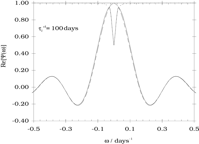
   Figure I.1: Real component of the transfer function (the gain) of the $\sigma=4000$ km s^-1 intensity component (solid line) as a function of excitation frequency $\omega$ assuming cloud equilibrium times of $\tau^{{\scriptsize\rm cl}}_{l}=100$ days. Also shown are the gains of the transfer functions of the individual clouds (dotted line) and the spatial gain (dashed line). This is for a hypothetical optically thin line using a very simple model, with a black hole of mass $M_{{\scriptsize\rm h}}=10^{8}~{}M_{\odot}($selected to yield a spatial time scale of $\tau^{{\scriptsize\rm sp}}=GM_{{\scriptsize\rm h}}/[3c\sigma^{2}]=10$ days). For $|\omega|<\omega_{l{\scriptsize\rm c}-}\simeq(30$ days$)^{-1}$, the spatial transfer function is approximately its asymptotic value. This defines the fast spatial regime. Conversely, for $|\omega|\mathrel{\hbox{\hbox to0.0pt{\hbox{\lower 5.0pt\hbox{$\sim$}}\hss}\hbox{$>$}}}\omega_{l{\scriptsize\rm c}+}\simeq(30$ days$)^{-1}$, the cloud transfer function is approximately its instantaneous value. This defines the slow cloud regime.

   , the spatial, cloud, and global (directly observable) intensity gains of an optically thin line of a spherically symmetric linear system are shown at a velocity dispersion of $\sigma=4000$ km s^-1. The line emitted by the clouds of this hypothetical model responds on an equilibrium time scale of $\tau^{{\scriptsize\rm cl}}_{l}=100$ days, with $\eta(F^{{\scriptsize\rm cl}}_{l}|F_{{\scriptsize\rm c}})=0.5$ and $\tilde{\hat{\Psi}}_{F^{{\scriptsize\rm cl}}_{l}|F_{{\scriptsize\rm c}}}(\infty)=1.0.$ (Such numbers might exist, for example, in a model with a linearly-responding line and large clouds that eventually evaporate when exposed to additional continuum heating.) The black hole mass is $10^{8}~{}M_{\odot}$, which was selected such that $\tau^{{\scriptsize\rm sp}}{\scriptsize\rm=}GM_{{\scriptsize\rm h}}/(3c\sigma^{2})=10$ days. The time constant ratios of this hypothetical model differ enough that the excitation frequency range of the intermediate regime is small. The fast spatial regime occurs here for $|\omega|<\omega_{l{\scriptsize\rm c}-}\simeq(30$ days$)^{-1}$, where the spatial intensity gain factor is approximately its asymptotic value of unity. In Figure I.2

   

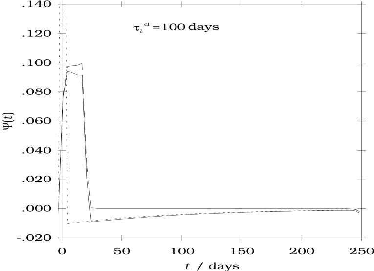
   Figure I.2: Time domain equivalents (response functions) of the system shown in Fig. I.1. An analog of the fast spatial regime occurs in the time domain on time resolution scales greater (poorer) than $\tau_{l{\scriptsize\rm c}+}=20$ days, while an analog of the slow cloud regime occurs on time resolution scales less (better) than $\tau_{l{\scriptsize\rm c}-}\simeq 30$ days. Note that the cloud response function is off the scale near zero lag. This is because $\tilde{\hat{\Psi}}_{F^{{\scriptsize\rm cl}}_{l}|F_{{\scriptsize\rm c}}}(\infty)$ is nonzero. Also, the solid (and easiest to measure) line has structure on a time scale much greater than the spatial response time scale, which indicates either a highly arranged distribution of matter or (via eq. [I.6]) locally delayed response. Unless specific deconvolution techniques were employed to avoid it, the empirical intensity component would have a nonzero width in dispersion space due to finite sampling resolution. This would result in a steep, rather than infinite, slope near $\tau=20$ days for such a hypothetical system. There is some numerical error at high and low values of $\tau$.

   , the response functions of this system are shown. For lags greater than $\tau_{l{\scriptsize\rm c}+}=20$ days, the global line intensity response function is equal to the cloud response function. By ignoring oscillations with frequencies above $\omega_{l{\scriptsize\rm c}-}$ and subtracting off either narrow or broad components of the line profile, this fast spatial regime is in principle always achievable for simple enough systems (that, e.g., are moderately spherically symmetric). However, as forewarned above, doing this in practice could be difficult or even impossible if, e.g., $\eta(\tau^{{\scriptsize\rm cl}}_{l}|r)$ is close enough to unity and $\sigma_{l{\scriptsize\rm c}+}$ is too high or $\sigma_{l{\scriptsize\rm c}-}$ is too low compared to the mean velocity dispersion in the observed line.

2. The “slow cloud” regime. In this case, $|\omega|\gg\omega^{{\scriptsize\rm cl}}_{l}$ yet $|\omega|\sim\omega^{{\scriptsize\rm sp}}$, which also requires $\tau^{{\scriptsize\rm cl}}_{l}\gg\tau^{{\scriptsize\rm sp}}$. This regime is the same as that illustrated in Figure I.1, but for $|\omega|>\omega_{l{\scriptsize\rm c}+}\simeq(30$ days$)^{-1}$, wherein the cloud gain factor is approximately its instantaneous value. Because this instantaneous gain is nonzero, the global intensity response function is approximately the product of the instantaneous cloud gain and the spatial response function for lags below $\tau_{l{\scriptsize\rm c}-}\simeq 30$ days.

3. The “slow spatial” regime. In this case, $|\omega|\gg\omega^{{\scriptsize\rm sp}}$ yet $|\omega|\sim\omega^{{\scriptsize\rm cl}}_{l}$, which requires $\tau^{{\scriptsize\rm cl}}_{l}\ll\tau^{{\scriptsize\rm sp}}$. In Figure I.3

   

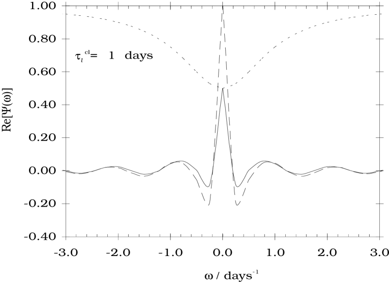
   Figure I.3: Real component of the transfer function of the $\sigma=4000$ km s^-1 intensity component assuming cloud equilibrium times of $\tau^{{\scriptsize\rm cl}}_{l}=1$ day. Other parameters are unchanged from those assumed in Fig. I.1. For $|\omega|\gg(3$ days$)^{-1}$, the intensity gain oscillates about zero. This is due to the spatial gain factor being near zero at high frequencies. This defines the fast spatial regime. For $|\omega|<\omega_{l{\scriptsize\rm c}-}\simeq(3$ days$)^{-1}$, the cloud gain factor is approximately constant. This defines the fast cloud regime.

   the gains are shown for a system like that of Figures I.1 and I.2 but for a hypothetical model in which $\tau^{{\scriptsize\rm cl}}_{l}=1$ day and $\tau^{{\scriptsize\rm sp}}{\scriptsize\rm=}10$ days. For $|\omega|\gg(3$ days$)^{-1}$ the intensity gain oscillates about zero because the instantaneous spatial intensity gain is zero for this model. This defines the fast spatial regime. In the time domain we see this regime on resolutions better than $\tau_{l{\scriptsize\rm c}-}\simeq 20$ days, where the derivative of the global intensity response function is equal to the cloud response function divided by the spatial response function at zero lag (see Fig. I.4

   

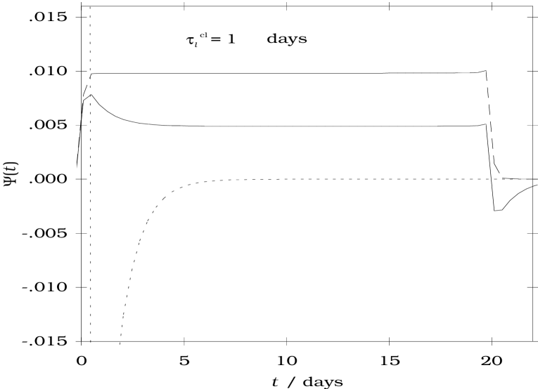
   Figure I.4: Time domain equivalents of Fig. I.3. Note that, as in Fig. I.2, the solid line has structure on two distinct time scales.

   .)

4. The “fast cloud” regime. In this regime, $|\omega|\ll\omega^{{\scriptsize\rm cl}}_{l}$ yet $|\omega|\sim\omega^{{\scriptsize\rm sp}}$, which also requires $\tau^{{\scriptsize\rm cl}}_{l}\ll\tau^{{\scriptsize\rm sp}}$. In the time domain this regime corresponds to lags greater than $\tau_{l{\scriptsize\rm c}+}$, where, as in the slow cloud case, the global response function is (within a time resolution of $\tau_{l{\scriptsize\rm c}+})$ approximately the spatial response function multiplied by the asymptotic cloud gain. This regime is illustrated in Figures I.3 and I.4, where $\omega_{l{\scriptsize\rm c}-}\simeq(3$ days$)^{-1}$ and $\tau_{l{\scriptsize\rm c}+}\simeq 3$ days. If $\eta(\tau^{{\scriptsize\rm cl}}_{l}|r)\sim 0,$ this fast cloud regime can be realized if the broader profile components with dispersion velocities above $\sigma_{l{\scriptsize\rm c}-}$ are subtracted out. Incidentally, in some prior work in which the fast cloud regime was apparently assumed, only narrow components were subtracted out (e.g., Krolik et al. 1991).

I.3 Applications and Model Fitting

The previous section contains mathematical expressions for the cloud and spatial transfer functions. It raises two questions. First, how, specifically, might such equations be used to make real measurements of the cloud and spatial response functions? Second, what specific benefits would this offer over the simpler methods of data analysis that have been employed in the past?

Analysis of variability data permits two potential benefits:

• It permits a reduction in the uncertainties of the values of the physical parameters that are used to fit a given object as defined within the context of the specific models that are fit. Note that these physical parameters have no meaning outside the specific models to which they are associated. Thus, any truly model-independent analysis of data would offer no new physical information about the system being observed.

• It permits a reduction of the uncertainty of the overall viabilities (i.e., goodnesses) of the models being fit provided the actual effective number of these parameters that have been granted to a model is small enough compared to that of the data.

Therefore, if local delays or nonlinearities are important, not only will the linear models that have traditionally been used in the past fail when they are not given excessive freedom, but also the values of the parameters obtained upon fitting such models will have little physical meaning. Since current theoretical and observational constraints are suggestive that local delays are important, we unfortunately need to employ models that can account for these effects in order to gain physical information from variability data. This subsection takes a step in this direction by presenting some models which are capable of accounting for local delays or nonlinearities.

From an experimental perspective, there is a simple way the equations of the prior section can be used. First, the various functions in the equations can be parameterized. Second, differences between the two sides of each equation can be assigned to difference variables. Third, the model parameters can be numerically adjusted within the constraints dictated by their error limits until the difference variables have been minimized. Before using any of the various software programs that have been written to perform this type of task, one must first select a compatible parameterization scheme for the model to be tested. The numerous parameters associated with certain models (such as those represented by eq. [F.4]) might be poorly constrained from the limited data and available information. In particular, if the only input knowledge for such a model is a linearized velocity-resolved response function, the various model parameters might not be uniquely determined, even if the observational errors were negligible. This is analogous to the shadow of an object not uniquely determining its topology unless, for example, the object is assumed to be both two-dimensional and viewed perpendicularly. For this reason, let us first consider the fitting of relatively simple models.

I.3.1 A Simple Linear Example Model

One of the simplest nontrivial models one could construct assumes instantaneous response, linearity (which under most circumstances implies that the effective cloud area A and line efficiency $\epsilon_{l}$ are independent of flux and hence radius), spherical symmetries in $f$ with respect to ${\bf r}$ and ${\bf v}$, and $\epsilon_{\hbox{{\scriptsize\rm A}{\scriptsize\it l}}}=0$. This last assumption would probably be applicable for lines suspected of having low optical depths, such as C III$]~{}\lambda 1909$. One way this model could be parameterized is by letting $f$ be an interpolation of a two-dimensional grid in $r$ and v with a resolution dictated by the quality of the data used. In this case, $f$ is constrained from the ionizing continuum flux $F_{{\scriptsize\rm c}}(t)$ and the observed spectrum $F_{\lambda}(t)$. Specifically, it is straightforward to show that

$$A\epsilon_{l}f(r,v)={r\over\pi c}{d^{2}\Psi_{F_{l}|F_{{\scriptsize\rm c}}}(2r/c,v)\over drdv}.$$ (I.11)

In this equation, $\Psi_{F_{l}|F_{{\scriptsize\rm c}}}(\tau,v_{{\scriptsize\rm D}})$ can be obtained (i.e., measured) from the linearized response function $\Psi_{F_{\lambda}|F_{{\scriptsize\rm c}}}$ of the spectrum $F_{\lambda}$ with respect to the ionizing flux $F_{{\scriptsize\rm c}}$, the convolution equation, and

$$\sum_{l}{c\over\lambda_{l}}F_{l}{\hbox{\bf(}}t,c(\lambda-\lambda_{l})/\lambda_{l}{\hbox{\bf)}}\simeq F_{\lambda}(t)-F_{{\scriptsize\rm c\lambda}}(t),$$ (I.12)

where $F_{{\scriptsize\rm c\lambda}}$ is the time-dependent spectrum of just the continuum. Use of the above equation in the overall fitting routine with $\epsilon_{l}$ being free parameters is important because profile de-blending, like any other interpretation of data, is necessarily model dependent, at least to some extent.

In Blandford & McKee (1982) a clear distinction is made between model fitting and blind mathematical fitting of a $\Psi_{F_{l}|F_{{\scriptsize\rm c}}}(\tau,v_{{\scriptsize\rm D}})$ function. However, note that equation (I.11) implies that a blind mathematical fitting of a response function to variability data of a given line is almost equivalent to model fitting of the arbitrary ${\it A\epsilon}_{l}f$ function above. In fact, other than the required transformation of variables (described in this case by eq. [I.11]) and their associated uncertainties, there is only one difference between model fitting using an arbitrary but linear model and fitting with an arbitrary linearized response function: with the latter method no physical significance is explicitly attached to the fitted function. Exactly what is considered here to be the “fundamental” set of parameters of a model selected for fitting is unimportant, provided that the measurement errors are also transformed appropriately.

However, this is not the case when more than one line is available. Because A and $\epsilon_{l}$ must be constants in the above linear model, the response functions for each line are proportional to one another. Thus, provided the local continuum flux determines the cloud properties, the mere fact that the response functions obtained by Krolik et al. (1991) appear to be line-dependent empirically tells us that the linearity assumption (in addition to this model) is formally incorrect. This tells us that the use of nonlinear models is probably necessary for fully self-consistent interpretations of AGN variability data.

I.3.2 A Simple Nonlinear Example Model

As a second example of a model that could be used in fitting, let us assume nonlinearly responding clouds with $F^{{\scriptsize\rm cl}}_{l}\propto F^{\eta_{l}}_{{\scriptsize\rm c}}$, where $\eta_{l}$ is an abbreviation for $\eta(F^{{\scriptsize\rm cl}}_{l}|F_{{\scriptsize\rm c}})$. Let us also assume that the other model parameters are the same as for the prior example model. This second example system has instantaneous (without delay) nonlinearities. Its exact nonlinear profiles are

$$F_{l}(t,v_{{\scriptsize\rm D}})=F^{{\scriptsize\rm cl}}_{l0}\int d\tau\left({F_{{\scriptsize\rm c}}(t-\tau,{\bf D})\over<F_{{\scriptsize\rm c}}>}\right)^{\eta_{l}}\hat{\Psi}_{F_{l}|F^{{\scriptsize\rm cl}}_{l}}(\tau,v_{{\scriptsize\rm D}}),$$ (I.13)

where

$$\hat{\Psi}_{F_{l}|F^{{\scriptsize\rm cl}}_{l}}(\tau,v_{{\scriptsize\rm D}})=2\pi r_{0}c\Theta(\tau)\int^{\infty}_{c\tau/2}dr\left({r\over r_{0}}\right)^{1-2\eta_{l}}n(r)\phi_{l}(\sigma,v_{{\scriptsize\rm D}})\hbox{ }$$ (I.14)

are “input-modified response functions” similar to the one in Maoz (1992).

If $\eta_{l}$ is forced to be independent of radius, it can be measured by fitting equation (I.13) to spectra. This method of obtaining the mean nonlinearities in the lines should be significantly more accurate than that in, e.g., Pogge & Peterson (1992), where the spatial response function was crudely approximated to be a delta function in lag.

The dependence of the kernel of an input-modified response function is a function of only lag $\tau$ via $\theta_{rs}\equiv\cos^{-1}(\hat{{\bf r}}\cdot\hat{{\bf s}})=\cos^{-1}(1-c\tau/r)$. If the dependence of $F^{{\scriptsize\rm cl}}_{l}$ upon $\theta_{rs}$ and $\hat{{\bf v}}$ is known then the local line profiles can be numerically fit from the velocity-resolved response functions. For instance, in this second example model we assume isotropic cloud line fluxes which yields (via eq. [I.14])

$$\phi_{l}(\sigma,v_{{\scriptsize\rm D}})={d\Psi_{F_{l}|F^{{\scriptsize\rm cl}}_{{\scriptsize\rm c}}}(\tau,v_{{\scriptsize\rm D}})/d\tau\over d\Psi_{F_{l}|F^{{\scriptsize\rm cl}}_{{\scriptsize\rm c}}}(\tau)/d\tau}|_{\tau=2GM_{{\scriptsize\rm h}}/(3c\sigma^{2})},$$ (I.15)

where the denominator is the integral of the velocity-resolved response function. With the above equations, the other physical properties such as $n(r),r_{0},F^{{\scriptsize\rm cl}}_{l0}$, and $M_{{\scriptsize\rm h}}$ can be measured within the context of this model.

Equation (I.15) is actually of little practical utility since the local profiles can be obtained in a more direct fashion by numerically fitting equations (I.13)-(I.14) to variability data. Equation (I.15), however, illustrates an important point. The equation would apply even if $\eta_{l}$ were a function of radius and the responses were very nonlinear. One assumption it does require is instantaneous responses from the clouds. Recall that the first example model illustrated that if there are line-dependent response functions than at least one of the cloud line emission functions is non-linear for models in which the emission is a function of only the local continuum flux. Here we see that if there is also a line dependence in the local profiles then either the assumption about the dependence of $F^{{\scriptsize\rm cl}}_{l}$ upon $\hat{{\bf r}}$ or $\hat{{\bf v}}$ is invalid or local delays are important. In the latter case, models like the second example model would fit the data poorly, yield low goodnesses, and give large measurement errors.

I.3.3 A Simple Example Model with Local Delays

As a third example illustrating how local delays and nonlinear response could be accounted for, let us assume the cloud areas and pressures have non-zero equilibrium times of $\tau_{P}(\sigma)=\tau_{P0}(\sigma_{0}/\sigma)^{2\eta(\tau_{P}|r)}$ and $\tau_{A}(\sigma)=\tau_{A0}(\sigma_{0}/\sigma)^{2\eta(\tau_{A}|r)}$. In the simplest case, these local delays can be parameterized with a linear model, with individual cloud line flux gains of

$$\tilde{\hat{\Psi}}_{F^{{\scriptsize\rm cl}}_{l}|F_{{\scriptsize\rm c}}}(\omega,{\bf r},{\bf v},\hat{{\bf s}})=1+{\eta(A|F_{{\scriptsize\rm c}})\over 1+i\omega\tau_{A}(\sigma)}+{\eta(\epsilon_{l}|F_{{\scriptsize\rm c}})\over 1+i\omega\tau_{P}(\sigma)}.$$ (I.16)

Let us again assume for this third example model that $\epsilon_{\hbox{{\scriptsize\rm A}{\scriptsize\it l}}}=0$ and that

$$f(r,v)=n(r){e^{-v^{2}/2\sigma^{2}}\over(2\pi\sigma^{2})^{3/2}},$$ (I.17)

where $n$ is the number density of clouds, with $\sigma^{2}=(r_{0}/r)\sigma^{2}_{0}$ and $\sigma^{2}_{0}=GM_{{\scriptsize\rm h}}/(3r_{0})$ so that $<{\bf v}^{2}>~{}\simeq GM_{{\scriptsize\rm h}}/r$ in accordance with a Maxwellian distribution of clouds. As mentioned in Appendix J, equation (I.17) is probably not as “square-shaped” in velocity space as certain theoretical models would suggest. However, it has the advantage of being built into most fitting packages. Equation (I.2) implies

$$\phi_{l}(\sigma,v_{{\scriptsize\rm D}})={e^{-v^{2}_{{\scriptsize\rm D}}/(2\sigma^{2})}\over\sqrt{2\pi}\sigma}.$$ (I.18)

This in turn permits measurement, without imposing instantaneous local response, of $I_{l}(t,\sigma)$ and $\Psi_{I_{l}|F_{{\scriptsize\rm c}}}(\tau,\sigma)$ when fit with equation (I.1), equation (I.12), and the convolution equation. In fact, for this model, equation (I.5) gives in the linear regime

$$\tilde{\hat{\Psi}}_{F^{{\scriptsize\rm cl}}_{l}|F_{{\scriptsize\rm c}}}(\omega,\sigma)=\omega\tau^{{\scriptsize\rm sp}}\tilde{\hat{\Psi}}_{I_{l}|F_{{\scriptsize\rm c}}}(\omega,\sigma){e^{i\omega\tau^{{\scriptsize\rm sp}}}\over\sin(\omega\tau^{{\scriptsize\rm sp}})},$$ (I.19)

which can be fit to equation (I.16) to measure $\tau_{P0}$, $\eta(\tau_{P}|r)$, $\tau_{A0}$, $\eta(\tau_{A}|r)$, $\eta(A|F_{{\scriptsize\rm c}})$, and $\eta(\epsilon_{l}|F_{{\scriptsize\rm c}})$ from time-resolved spectra. For more accurate modeling and lower measurement errors at the expense only of computation time, equation (I.16) could be replaced by a nonlinear analog. The point in either case is that the physical parameters of the model, including the cloud pressure equilibrium times, are indeed measurable quantities provided theoretical constraints can be imposed upon the angular dependence of $F^{{\scriptsize\rm cl}}_{l}$.

Note that this third example model does not necessarily have more degrees of freedom than the first two. This is because upon including the above six parameters, one would accordingly reduce the grid resolution of the fitted functions like $n(r)$ such that the effective number of parameters (e.g., the order of its polynomial) permitted in the model remained the same. Incidentally, this reduction would be small when the quality of data is high and the response functions can be interpolated from several points. Performing the computationally expensive nested integrals (such as those implicit in the line flux equation of models with local lags) instead of the linear approximations (eq. [I.16]) admittedly provides a means of accounting for both nonlinear and inseparable behavior if sufficient computer time is available. In the linear regime, however, including parameters to account for finite response times in a cloud would not change the prediction error of the model at all.

In this context, as stated above, the real benefit of model fitting with $f$ and cloud lag parameters over “blind” mathematical de-convolution is that the fitted quantities have physical meaning. For instance, features in $\Psi_{F_{l}|F_{{\scriptsize\rm c}}}$ beyond lags of $4GM_{{\scriptsize\rm h}}/v^{2}_{{\scriptsize\rm D}}c$ would be physically meaningful in the third example model provided that the equilibrium times scale of at least one cloud property is sufficiently long. Similarly, additional information, such as that from fully nonlinear photoionization codes like CLOUDY, XSTAR, ION, etc. can be included (albeit with substantial systematic error) along with the line emission data to lower the errors of the fitted parameters. This would, for example, help exclude so-called “unphysical de-convolutions.” Also, if one is fitting the underlying physical conditions of the gas emitting the lines rather than the line emissivities themselves, line blending aids and constrains our knowledge of what we are fitting (as opposed to hindering it). With abstract mathematical de-convolution, valuable information resources like these must be thrown away. (Invoking physical arguments to interpret an abstract de-convolution is a crude means of model fitting. This point, along with others on the advantages that model fitting has over “arbitrary” function fitting, is discussed in more detail elsewhere.) Though linear response functions or, for the apparently nonlinear cases, even multidimensional “time-dependent” response functions might be able to fit variability data well, they probably do not offer as much to our understanding of AGNs as does model fitting.

I.4 Conclusion & Discussion

This appendix discusses the analysis of AGN spectral variability data using line emission models that have “reactive” clouds in orbital motions. For such models, the line intensity representation of the line profiles is useful for obtaining the cloud response characteristics. These response characteristics are simplest when their transfer functions are “separable” from the spatial transfer functions of the intensities. A total of four different separable regimes are possible. For spherical systems without occulting material, the observed linearized response function of the intensity is a trapezoidal function only in the fast and slow cloud regimes. If the characteristic cloud equilibrium time or frequency is a weak enough function of the mean local continuum flux, the fast cloud regime would occur at excitation frequencies significantly lower than the characteristic equilibrium frequency for components of the intensity with low enough velocity dispersions. In the same such system, the slow cloud regime would occur at excitation frequencies significantly above the characteristic equilibrium frequency at high enough velocity dispersions. Even outside these simplifying regimes of separability, nature permits, under certain assumptions, measurement (via, e.g., eq. [I.5]) of the linearized response functions of clouds at a given position. However, these types of measurements would require variability data with much larger duration to sampling period ratios than would be necessary in the fast cloud regime.

Abstract mathematical deconvolution discussed in Blandford & McKee (1982) is probably not the ideal method of analyzing variability data. If its purpose were merely to predict variability data, then other fully nonlinear methods, such as those employed with neural nets to predict, e.g., stock prices, would probably fare better. If, on the other hand, the ultimate goal is to increase our knowledge of the physics of the AGNs, then the model fitting discussed in Blandford & McKee (1982) would probably fare better; only model fitting permits measurement of several parameters within the context of specific models while formally accounting for their physical plausibility. For instance, the example model of § I.3.2 can be used to measure the mean asymptotic gain $\eta(F_{l}|F_{{\scriptsize\rm c}})$ of a line without approximating the spatial response function to be a delta function in lag as was done in previous works (Krolik et al. 1991; Pogge & Peterson 1992). Another set of parameters is the linearized response function of the intensity in a line with respect to the continuum flux $\Psi_{I_{l}|F_{{\scriptsize\rm c}}}$. When information from a photoionization code is included in the fitting of a model, this function would probably be of more utility than $\Psi_{F_{\lambda}|F_{{\scriptsize\rm c}}}$. This is because the range of cloud parameters sampled by the intensity at a given velocity dispersion is much smaller than that sampled by the linearized spectral response function at a given wavelength.

It is the knowledge of the values of the various physical parameters that can help us understand AGNs. For instance, knowledge of the radii in a fitting of a model that incorporates fully nonlinear results (e.g., $\epsilon_{l})$ from a photoionization code where contributions to the reduced $\chi^{2}$ are large would help indicate the parameter space wherein more physics is necessary and uniform pressure cloud models fail. Knowledge of which lines have behavior that is inconsistent with the black hole mass inferred from other lines, after nonlinear behavior is taken into account, would give an independent upper limit to how important alternative line broadening mechanisms (e.g., electron scattering) could be in orbital models. Knowledge of the sign of $\eta(A_{\hbox{{\scriptsize\rm geom}}}|F_{{\scriptsize\rm c}})$, where $A_{\hbox{{\scriptsize\rm geom}}}$ is the geometrical size of the clouds, would help answer the very important question of whether or not the source of clouds in AGNs, which has been debated since their introduction, is in part due to the continuum flux or just some passive element of the overall AGN environment.

Perhaps the most important knowledge that can be gained by proper model fitting is that related to the cloud response functions $\Psi_{F^{{\scriptsize\rm cl}}_{l}|F_{{\scriptsize\rm c}}}$. For instance, consider that the emission efficiency in a line can drop significantly when the column density to ionization parameter ratio becomes low enough that the “back” portions of a cloud are too highly ionized for significant emission by an ion. Partly for this reason, intensity line ratios could be used to obtain measurements of mean column densities as a function of radius (along with the pressures or densities). This in turn could permit measurement of cloud characteristics such as the time-averaged size of the clouds as a function of radius. With cloud response functions, the time-dependence of these various cloud properties can also be determined, which would permit measurement of the cloud evaporation and pressure-equilibrium wave propagation speeds (even if they are nearly zero). Such knowledge would impose new and important constraints upon the various cloud confinement mechanisms that have been proposed.

Rather than be distressed that nature is more complicated without the fast cloud assumption, we should consider ourselves very fortunate, for cloud response functions would allow us to directly probe the structure of an individual cloud within the context of a model, and, if the cloud concept is valid, help answer the question “What are the clouds?” Answering this question, rather than “Where are the clouds?” is probably more important for understanding AGNs.

Appendix J Obtaining the Local Line Profiles

According to Appendix I, a priori knowledge of both the local line profiles $\phi_{l}$ and the distance from the black hole $r$ as a function of velocity dispersion parameter $\sigma$ is necessary before measurements of the intensities can be made from a spectrum. This appendix discusses issues relating to how these two quantities might be constrained.

As the example model discussed in § I.3.2 illustrates, the local line profiles should be particularly straightforward to measure if the following assumptions are valid:

1. the local line shifts (which velocity-dependent emission can cause) are negligible,

2. the velocity dispersion function $r(\sigma)$ is known,

3. a velocity-resolved input-modified response function can be measured for at least one line,

4. the approximate dependence of $F^{{\scriptsize\rm cl}}_{l}$ upon $\theta_{rs}\equiv\cos^{-1}(\hat{{\bf r}}\cdot\hat{{\bf s}})$ is known, and

5. the clouds respond instantaneously (i.e., without “hysteresis”).

Because of the normalization condition imposed upon $\phi_{l}$, condition (1) would yield the local profiles to be identical for each line. When this is not the case, the line flux can also be projected into velocity shift space. Condition (2) is satisfied by $r(\sigma)=GM_{{\scriptsize\rm h}}/(3\sigma^{2})$, which should be applicable in the BLR of the orbital models of interest here. Condition (3) holds provided the sampling resolution is high enough and the local continuum flux determines the properties of the clouds (even if the system is nonlinear). Condition (4) can be partially met if we apply photoionization codes to determine the approximate beaming factors $\epsilon_{\hbox{{\scriptsize\rm A}{\scriptsize\it l}}}$, we assume a spherically symmetric cloud density function, and we assume a specific absorption model or simply assume that absorption is unimportant. The validity of condition (5) is questionable, but could at least be tested if the conditions (1)-(4) are met by comparing the local profiles of various lines (§ I.3.2).

For the more general cases in which any of the above conditions are not met, further constraints upon the local profiles can be made by again exploiting the orbital motions assumption, which states that the clouds are accelerated purely by gravitational interactions. From this assumption, the only distinguishing characteristic relevant to the distribution function is the particle mass. This is the same primary assumption that is used to determine stellar distribution functions. Therefore, provided the other characteristics of the clouds (e.g., the areas) do not affect the dynamics, the distribution function of the clouds (and local profiles that are functions of it) are proportional to those of stars with similar masses. Techniques used to constrain stellar distribution functions can then be employed.

One common assumption made in working with stellar distribution functions is that the collision rate is zero, or $df/dt=0.$ In this case, provided the relaxation time is short enough compared to the age of the galactic nucleus, the distribution function is purely a function of the isolating integrals of motion about the mean potential, such as the energy and angular momentum. For simple models that obey complete spherical symmetry, $f$ can only be a one-dimensional function of energy per unit mass E. This energy is a simple function of the cloud radius, velocity, and cloud number density function $n(r)$, which is proportional to the mass density $\rho(r)$ in the above circumstances. Therefore, because $f(E)$ is a one-dimensional function, it is a unique function of $n(r)~{}($see, e.g., discussion in Binney & Tremain 1987). For this reason, the local profiles can be calculated from the cloud number density $n(r)$ if the mass to cloud number density ratio is known.

For spherically symmetric models the non-velocity-resolved response function and the time-averaged profile of a line are functions of only the mean continuum flux and $A\epsilon_{l}(1+\epsilon_{\hbox{{\scriptsize\rm A}{\scriptsize\it l}}})n(r)$, where A is the cloud area function and $\epsilon_{l}$ is the dimensionless line efficiency. Therefore, provided the mass to cloud density and the dependencies of ${\it A},\epsilon_{l}$, and $\epsilon_{\hbox{{\scriptsize\rm A}{\scriptsize\it l}}}$ upon the local continuum flux are calculable, the non-velocity-resolved response function or the time-averaged profile of a line can be used to determine $f(E)$. With velocity-resolved response functions, $f(E)$ is therefore over-constrained if instantaneous response is assumed. On the other hand, if local delays are assumed the cloud response functions can be measured under these circumstances.

An analogous situation exists in galactic dynamics, with the one-dimensional angular brightness function taking the place of the response function. In this case, $f(E)$ can be deconvolved only if the mass to light ratio $M/L$ is known a priori. However, with velocity information, both the radial dependence of the $M/L$ ratio and $f(E)$ can be measured. Reverberation mapping is actually worse off in that not all of the parameters are measurable unless theoretical constraints are imposed upon some of the parameters; we can chose to measure either $A,\epsilon_{l}$, and dependence of $F^{{\scriptsize\rm cl}}_{l}$ upon angle by placing theoretical constraints upon the cloud response functions (e.g., nonlinear instantaneous response) or we can choose to measure the cloud response function parameters such as the pressure equilibrium time by placing theoretical constraints upon ${\it A},\epsilon_{l}$, and $\epsilon_{\hbox{{\scriptsize\rm A}{\scriptsize\it l}}}$. For the more complex and realistic models, $\sigma\propto r^{-1/2}$ merely becomes a very powerful constraint to be employed in doing numerical model fitting to equation (I.4).

As is typical of relaxed stellar systems, the local profiles that result from applying the above procedure under the assumption of instantaneous response resemble Gaussians at least to the first order. If $f$ is additionally a function of angular momentum, the local line profiles can have a position-dependent shift. However, the form of the un-shifted local profiles would probably remain somewhat Gaussian-like, in accordance with the $df/dt=0$ assumption. Note that such model-independence of the local profiles probably does not extend to the density functions, as it is primarily constrained by the macroscopic boundary conditions imposed upon $f$ rather than the relaxation time scale. In this case, the local line profiles can probably be assumed to be similar for all AGNs with clouds in orbital motions, with the density functions providing the primary object-to-object freedom in f.

More careful considerations show that the local line profiles of $df/dt=0$ systems must be more “square-shaped” than Gaussian. Physically, this occurs because of the constraints imposed upon f. For instance, with $df/dt=0,$ the cloud escape rate must be zero, with zero clouds having kinetic energies above the potential depth (unlike a Maxwellian distribution). In contrast, the observed profiles of lines with relatively constant emission efficiencies (lines similar to, e.g., Ly$\alpha$, which is probably emitted over a large range of radii) are “logarithmic.” Because of this fundamental difference in form, measurement of $I_{l}$ within the context of orbital models at several different points in $\sigma$-space should be possible via application of equation (I.1) to a given spectrum in which the profile of interest is resolved.

However, for some models, $df/dt\neq 0.$ This might occur if the cloud creation or physical collision rate is high enough, as is expected in very dense stellar systems. It might also occur at small radii for models requiring a $f({\bf 0},{\bf v})=0$ boundary condition. It is straightforward to show that if $f({\bf r},{\bf v})$ scales to a power of $r$ that is greater than $-{1\over 2}$ at small $r$, then $df/dt\neq 0,f$ is not positive-definite, or $f$ is not a function of energy alone. Consideration of such $df/dt\neq 0$ orbital cloud models are outside the scope of this work.

Appendix K Absorption Reverberation Mapping

K.1 Background

An estimated $10\%$ of all AGNs have line absorption features with strengths and widths approximately as large as their emission lines. Moreover, line profile observations at high resolution indicate blueshifted absorption features in about $50\%$ of Seyfert galaxies. Despite these facts, most of the theoretical work on AGNs to date, including the derivations shown in Chapter 2, neglects absorption.

In this appendix I discuss how absorption spectral features could be used to constrain absorption models. Although time-averaged line absorption features severely constrain absorption line QUASAR (BALQSO) models, here I will focus upon only analysis of time-dependent absorption data, or “absorption reverberation mapping.” It is well known that reverberation mapping using emission lines has been quite useful for constraining AGN line emission models. Unfortunately, studies analogous to these but for absorption spectral features have not yet been performed. In this appendix I show that absorption reverberation mapping appears to have at least as much potential for constraining absorption models as does emission mapping for AGN line emission models.

Though it is conceivable that the absorption mechanisms in BALQSOs are completely different in separate objects, the differences (e.g., not being radio loud, having a smooth dependence of the absorption characteristics upon luminosity, etc.) between BALQSOs and normal AGNs suggest that the absorption mechanisms in all AGNs may be inherently similar. Therefore, constraining models of AGNs with only modest absorption should help us understand BALQSOs as well. Moreover, because certain AGN models (e.g., Murray et al. 1995) make predictions about both the emission and absorption features, these constraints could also help us understand how line emission operates in AGNs.

The nearest BALQSO is NGC 4151. Partly for this reason most of the calculations in this appendix are scaled for this source. Observations of NGC 4151 have been obtained at the highest sampling frequency thus far; the 1993 intensive ultraviolet IUE reverberation mapping campaign of NGC 4151 (Edelson et al. 1993) had a sampling interval of only $\sim 70$ minutes. As I show in § K.4.1, this is the approximate time resolution that would be necessary in order to perform effective absorption reverberation mapping. I also show that absorption reverberation mapping requires velocity resolution at least as high as that of HST. For these reasons, currently available observations are inadequate for performing absorption reverberation mapping, and this appendix is an attempt to see what results the analysis of AGN data might yield in the future.

Broad absorption line quasar (BALQSO) absorption trough response time scales can be significantly less than the associated emission response time scales. Thus, accurate measurement of absorption delays in AGNs requires higher sampling frequencies than those used in emission line reverberation studies. For instance, data obtained of NGC 5548 from the HST reverberation mapping campaign only permits measurement of an upper limit to the absorption response delay. This is shown in Figure K.1.

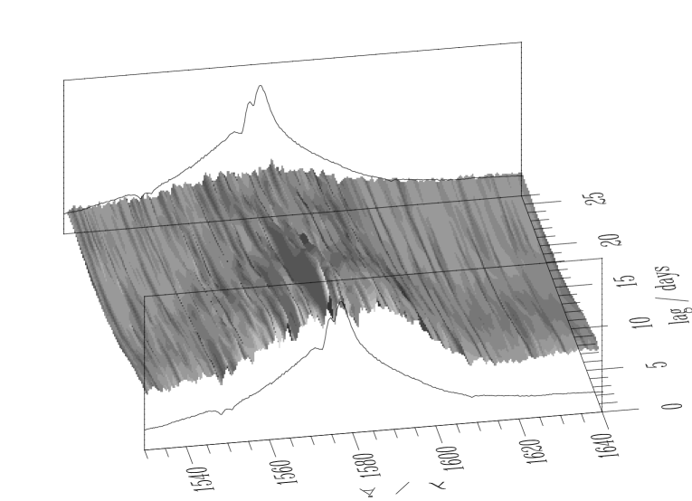
Figure K.1: The cross covariance function of the $1135-1180\hbox{\rm\AA}$ de-redshifted continuum with respect to the spectra of NGC 5548 using the HST variability campaign data. A weak blueshifted C IV absorption doublet feature is evident even in this non-BAL Seyfert. The cross covariances of the absorption features have a width in delay space that is approximately equal to the sampling rate of $\sim 3$ days. This result is expected for both accelerating and decelerating outflow models obeying equation (K.1) in §K.2. Therefore, despite the excellent wavelength resolution of HST, this data set is not particularly useful for mapping the absorption trough response functions and directly distinguishing between the accelerating and decelerating classes of absorption models.

K.2 Estimates of Possible BALQSO Trough Response Characteristics

Unlike the delays of emission lines, delays in changes of absorption trough depths in response to changes in continuum levels are not proportional to the distance of the line-affecting gas from the continuum source. Several papers have stated that delays in absorption trough depths cannot reveal any information about the positions of the absorption clouds except indirectly via the implied lower limits to the recombination time scales (e.g.; Voit, Shull, & Begelman 1987; Barlow 1994). This conception is essentially valid for absorption of the continuum component of the spectrum. It is invalid, however, for absorption of the line emission component of the spectrum for the BALQSO models that are currently favored. This is shown in the following.

Figure K.2: Generic BALQSO model. The slab of the absorbing medium shown has an outflow speed of $v_{r}$. Though the cross-sectional area of the slab absorbing continuum radiation at a wavelength of $\sim\lambda_{l}(1-v_{r}/c)$ is relatively small, the cross-sectional area of the slab absorbing line emission radiation is ${\it r}^{2}_{{\scriptsize\rm e}}$.

BALQSO absorption trough components generally appear to be blueshifted with respect to the emission components. In most BALQSO models, these blueshifts occur because the absorbing material is assumed to be outflowing in radial motion away from the continuum source and toward the observer. Thus, BALQSO models are similar to P Cygni stellar wind models. The BALQSO model is shown in Figure K.2. The emission region shown has a non-zero scale size of $r_{{\scriptsize\rm e}}\simeq c/\tau_{{\scriptsize\rm e}}$, where c is the speed of light and $\tau_{{\scriptsize\rm e}}$ is a mean response time scale of the emission region that is presumably measurable from emission variability analysis. (A more general and precise analysis accounting for a large range of emission radii, for instance, could be performed but is unnecessary for our purposes here.) Though the continuum absorption region is assumed to be much smaller than the emission region, note that the cross-sectional area of the absorption region is the same as that of the line emission region. The differential path length gives the relative time delay for the observed absorption trough component to respond to changes in the continuum flux due to the dependences of the optical depths of the absorbing clouds upon the ionization parameter,

$$\tau_{{\scriptsize\rm a}}\simeq{r_{{\scriptsize\rm a}}\over c}\left(\sqrt{1+r^{2}_{{\scriptsize\rm e}}/r^{2}_{{\scriptsize\rm a}}}-1\right)+\tau_{{\scriptsize\rm r}}.$$ (K.1)

In this equation, $r_{{\scriptsize\rm a}}$ is the distance of the absorbing gas from the continuum source and $\tau_{{\scriptsize\rm r}}$ is the ionizational equilibrium time scale, which includes the recombination time. Given a functional dependence of the outflow velocity $v_{r}$ upon radius $r_{{\scriptsize\rm a}}$, equation (K.1) gives the delay as a function of the equivalent line-of-sight velocity $v\simeq-v_{r}\simeq c(\lambda-\lambda_{l})/\lambda_{l}$, where $\lambda$ is the wavelength and $\lambda_{l}$ is the wavelength of the line center. Since absorption of line emission requires $r_{{\scriptsize\rm a}}>r_{{\scriptsize\rm e}}$, for the $\tau_{{\scriptsize\rm r}}\ll\tau_{{\scriptsize\rm a}}$ case equation (K.1) implies $\tau_{{\scriptsize\rm a}}<\tau_{{\scriptsize\rm e}}$. Therefore, for the purposes of determining the velocity dependence of the approximate minimum absorption response time scale, time dependence of the line emission variation can be neglected for $\tau_{{\scriptsize\rm r}}\ll\tau_{{\scriptsize\rm a}}$ models.

Equation (K.1) indicates that there are three different classes of models distinguishable via their velocity dependence of the absorption trough response minimum variation time scale:

• “Accelerating outflow models” in which the outermost absorbing clouds, for some reason, are moving the fastest.

• “Decelerating outflow models” in which the innermost absorbing clouds are moving the fastest.

• “Detached models” in which the gas density is low enough that the recombination time provides the dominant contribution towards the total delay.

Let us discuss each of these model classes in turn.

For accelerating models, $v_{r}$ increases as $r_{{\scriptsize\rm a}}$ increases. Therefore, if $\tau_{{\scriptsize\rm r}}\ll\tau_{{\scriptsize\rm a}}$, equation (K.1) implies that $\tau_{{\scriptsize\rm a}}$ increases as v increases for this model, with the blue side of the absorption trough having a smaller minimum response time scale than the red side of the absorption trough.

For the decelerating class of models, $\tau_{{\scriptsize\rm a}}$ decreases as v increases. In this case the red side of the absorption trough should be able to respond first.

A further division between classes of outflow models can also be made. If the acceleration mechanism of the outflow is such that the terminal outflow velocity is comparable to the gravitational escape velocity, the radial absorption slab velocity -v could, at least for some models, be used to estimate the relative distance to the continuum source. This permits estimates of $r_{{\scriptsize\rm a}}$ for such models. In particular, for such gravitationally regulated outflow models,

$$r_{{\scriptsize\rm a}}\sim r_{{\scriptsize\rm e}}(v_{{\scriptsize\rm e}}/-v)^{2},$$ (K.2)

where $v_{{\scriptsize\rm e}}$ is a velocity scale of the underlying emission line. From crude estimates of the absorption ionization parameter $U_{{\scriptsize\rm a}}$ based upon absorption optical depth ratios, estimates of the hydrogen density $n_{{\scriptsize\rm H}}$ and corresponding recombination times $\tau_{{\scriptsize\rm r}}$ for certain gravitationally regulated outflow models can be made. The densities in AGN emission line regions are suspected to be high (e.g., $n_{{\scriptsize\rm H}}\sim 10^{11}$ cm${}^{-3})$. Therefore, because BALQSO absorption trough widths are comparable to the FWHM of the emission profiles, equation (K.2) implies that the absorption recombination times are small in gravitationally regulated outflow systems. Conversely, recombination could be the dominant contributor toward delay $\tau_{{\scriptsize\rm a}}$ in “detached outflow systems.” Such detached systems should be different from the gravitationally regulated outflow systems in that the absorption of the continuum radiation emitted near a resonance line and the absorption of the line emission itself should respond on the same time scale (the recombination time).

Figure K.3: Approximate minimum delays in the response of the mean line and continuum absorption components to changes in continuum flux for three models. The top graph gives the predicted delays for an accelerated outflow NGC 4151 absorption model. The solid line represents the approximate mean delay of the line absorption component, while the dotted line represents the approximate mean delay of the continuum absorption component. For this model, the continuum absorption delay (which is approximately the recombination time) is negligible at most velocities. The delay of the absorption component of the line emission is smallest on the blueward side of the absorption trough. The middle graph gives the predicted delays for the decelerating outflow class of BALQSO models. It predicts the opposite response behavior, with the blueward side of the absorption trough responding the fastest. Finally, the lower graph gives the predicted absorption trough response delays for detached outflow models. The gas density assumed at the innermost edge of the absorption region was $n_{{\scriptsize\rm H}}=6.6\times 10^{4}$ cm^-3. For this model, both line and continuum absorption components are predicted to respond on the recombination time scale, with the redward side of the absorption trough responding fastest.

These results are summarized by the calculations shown in Figure K.3. The top graph gives the absorption delay/velocity results that equations (K.1)-(K.2) yield for accelerating outflow, the middle graph gives the results for decelerating outflow, while the lower graph gives the results for detached accelerating outflow. These calculations are intended for NGC 4151; in accordance with results published in Ulrich & Horne (1996), they assume a characteristic emission delay of 4.4 days for the core emission component, 3.2 days for the blue emission wing, and $v_{{\scriptsize\rm e}}=2000$ km s^-1 for the underlying emission scale velocity. The calculations also assume a position-independent absorption ionization parameter of ${\it U}_{{\scriptsize\rm a}}=0.01.$ This value of ${\it U}_{{\scriptsize\rm a}}$ was selected to be as consistent as possible with values quoted in the literature, which include $U_{{\scriptsize\rm a}}\simeq 0.001~{}($Turnshek $1994),0.01\mathrel{\hbox{\hbox to0.0pt{\hbox{\lower 5.0pt\hbox{$\sim$}}\hss}\hbox{$<$}}}U_{{\scriptsize\rm a}}\mathrel{\hbox{\hbox to0.0pt{\hbox{\lower 5.0pt\hbox{$\sim$}}\hss}\hbox{$<$}}}0.07~{}($Hamann, Korista, & Morris 1993), and $U_{{\scriptsize\rm a}}\mathrel{\hbox{\hbox to0.0pt{\hbox{\lower 5.0pt\hbox{$\sim$}}\hss}\hbox{$>$}}}0.05~{}($Barlow 1995). Results similar to those shown in Figure K.3 are obtained with different absorption ionization parameters and with absorption gas pressures that are constant along the line of sight. In the detached accelerating outflow model, the density was assumed to drop as $v^{-1}_{r}r^{-2}_{{\scriptsize\rm a}}$. Therefore, in this model the redward side of the absorption trough responds before the blueward side. One prediction of the detached model that is different from the other two model classes is that it predicts the absorption of both the continuum and line emission components to be delayed by the same amounts (the recombination time).

K.3 Crude Predictions for Popular BALQSO Models

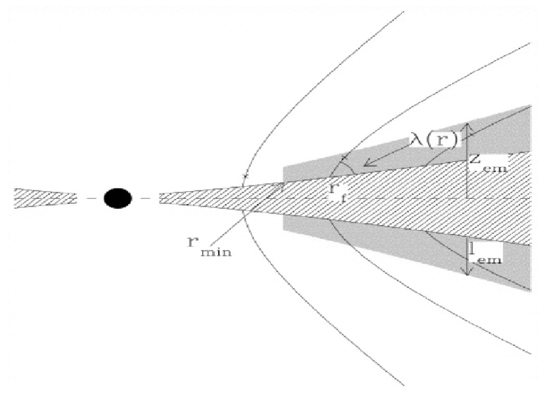
Figure K.4: The Murray, Chiang, Grossman, and Voit AGN/QSO model. At high inclination angles, absorption of line emission occurs. In such BALQSO cases, the absorbing gas farthest from the broad emission line region has the slowest line-of-sight velocity.

In a recent review article (Weymann 1995), three BALQSO models were discussed: the model of Murray et al. (1995), the model of Scoville & Norman (1995), and the model of Arav, Li, & Begelman (1994). In this section, we discuss each of these models in turn. We then attempt to estimate how these models should compare with the models shown in Figure K.3.

K.3.1 Murray, Chiang, Grossman, and Voit Disk Wind Model

The Murray et al. (1995) BALQSO model is shown pictorially in Figure K.4. This model assumes that the accretion disk surrounding the black hole has a radiatively accelerated outflowing wind with a shear velocity of the order of the radial velocity. In this model, $\sim 10\%$ of AGNs are BALQSOs because the opening angle of the wind is $\sim 81^{\circ}=(1-0.1)\times 90^{\circ}$. The mass loss flux is predicted to adjust itself such that the terminal wind velocity of a given stream line is comparable to the gravitational escape velocity (Murray, et al. 1995). Because of the non-radial shape of the streamlines, however, the absorbing gas farthest from the central source has the slowest tangential velocity. Therefore, this model is in many ways similar to the decelerating model shown in the middle of Figure K.3. Thus, the red side of the absorption trough should be able to respond faster than the blue side of the absorption trough in this model. However, this model is somewhat complex; more accurate calculations would be required before firmer predictions of this model could be made.

Incidentally, this model should have absorption response characteristics similar to other models in which the innermost clouds move faster than the outermost clouds and where the velocities are comparable to the escape velocities. In particular, this model should be similar to the model discussed in Appendix L.

K.3.2 Scoville and Norman Contrail Model

In the BALQSO model of Scoville & Norman (1995), “contrails,” or remnants of stellar winds, are slowly accelerated outward via radiation pressure. In this model, remnants with the highest radial velocity also have the highest mean $r_{{\scriptsize\rm a}}$. Moreover, the radial velocities are also associated with the escape velocities. With regard to the velocity dependence of the absorption trough component, this model falls into the accelerating class and the absorption trough response delay should be similar to that shown in the top of Figure K.3. Therefore, the bluest absorption trough components should have the shortest minimum response time scale and $\tau_{{\scriptsize\rm r}}\ll\tau_{{\scriptsize\rm a}}$.

For this model, there is a non-zero radial velocity dispersion at a given $r_{{\scriptsize\rm a}}$. For a BALQSO with an absorption equivalent width of 1000 km s^-1 and a maximum possible thermal/inter-contrail turbulent velocity gradient of 50 km s^-1, a lower limit to the number of separate optically thick contrails of maximal emission blocking region area $\sim r^{2}_{{\scriptsize\rm e}}$ is $\sim 1000/50=20\gg 1.$ Therefore, the probability that the essential red/blue absorption response behavior for this model is drastically different from that shown in the middle graph of Figure K.3 is probably small.

K.3.3 Arav, Li, and Begelman Clumpy Outflow Model

In this model, clumps of absorbing material are assumed to be outflowing in radial motion away from the continuum source. The densities are relatively low in this case because radiative acceleration is assumed to be high enough that the gravitation acceleration can be neglected (Arav et al. 1994). As a result, the terminal velocities of the winds are much higher than the gravitational escape velocities. This implies much larger values of $r_{{\scriptsize\rm a}}$ than in the other two classes of models. Because of constraints upon the ionization parameter, this in turn implies lower densities for the absorbing gas than for the other models. The densities assumed in the detached model of Figure K.3, however, are still approximately $10^{4}$ times lower than those assumed by Arav, Li, and Begelman (1994). Therefore, depending upon the particular values of parameters assumed, this model could behave either like the detached model or like the accelerating model shown in Figure K.3.

K.4 Requirements of Velocity and Temporal Resolution to Discriminate Between Popular BALQSO Models

Before any attempt is made to perform absorption reverberation, suitable data must be obtained first. In this section I make some crude estimates of the probably velocity and temporal resolution that would be required.

K.4.1 Velocity Resolution

In principle, the absolute minimum number of velocity components that would permit constraints to be imposed upon the BALQSO models is 2: a redward absorption trough component and a blueward absorption trough component. The NEWSIPS IUE SWP spectral resolution is one pixel per $1.6\hbox{\rm\AA}$ at $1550\hbox{\rm\AA}$. GHRS observations of NGC 4151 indicate that the C IV $\lambda 1548.2/1550.8$ broad line absorption trough is $\mathrel{\hbox{\hbox to0.0pt{\hbox{\lower 5.0pt\hbox{$\sim$}}\hss}\hbox{$>$}}}11\hbox{\rm\AA}$ wide (Weymann 1996). This implies $11/1.6\sim 7$ independent measurable IUE velocity absorption trough components. A more conservative (and probably more realistic) estimate assuming half this resolution would yield $\sim 3.4$ different velocity components. With random and fixed-pattern noise it could be even less.

Since $3.4\geq 2,$ it could be argued that IUE resolution might be sufficient to distinguish between the three classes of models discussed in this appendix. However, in order to produce an accurate, smooth velocity-resolved map of the linearized absorption trough response function, the much higher resolution of HST would probably be required.

K.4.2 Estimates of the Expected Sampling Rate and Temporal resolution

In a system that responds to input excitations with characteristic delay of $\tau_{{\scriptsize\rm a}}$, a conservative maximum effective sampling period required to place empirical lower limits upon $\tau_{{\scriptsize\rm a}}$ is $\mathrel{\hbox{\hbox to0.0pt{\hbox{\lower 5.0pt\hbox{$\sim$}}\hss}\hbox{$<$}}}\tau_{{\scriptsize\rm a}}/3.$ Similarly, in order to place upper limits upon $\tau_{{\scriptsize\rm a}}$, the data set must span a minimum time of $\sim 3\tau_{{\scriptsize\rm a}}$. In this section we show that for both the accelerating and decelerating classes of BALQSO models these two conditions can be met by data that are sampled at rates as high as or higher than that obtained in the 1993 IUE continuous monitoring campaign of NGC 4151 .

If the sampling time is less than the time required for the flux within the trough to change more than the $1\sigma$ uncertainty, the effective absorption trough flux sampling rate is

$$\tau_{{\scriptsize\rm a}1\sigma}\simeq{F_{{\scriptsize\rm a}}\over|\dot{F}_{{\scriptsize\rm a}}|}{\sigma_{F_{{\scriptsize\rm a}}}\over F_{{\scriptsize\rm a}}},$$ (K.3)

where $F_{{\scriptsize\rm a}}$ is the flux in or near the absorption trough, $\sigma_{F_{{\scriptsize\rm a}}}$ is its $1\sigma$ uncertainty, and $|\dot{F}_{{\scriptsize\rm a}}|$ is the amplitude of its typical derivative with respect to time. The $1275\hbox{\rm\AA}$ continuum flux change rate was $\mathrel{\hbox{\hbox to0.0pt{\hbox{\lower 5.0pt\hbox{$\sim$}}\hss}\hbox{$<$}}}10\%$ in several hours (Crenshaw et al. 1996). Therefore, if the asymptotic dependence of the transmission coefficient were to respond linearly upon variations in the $1275\hbox{\rm\AA}$ continuum flux, the effective sampling rate would be $\tau_{{\scriptsize\rm a}1\sigma}\sim 3$ hours.

For a more realistic estimate of $\tau_{{\scriptsize\rm a}1\sigma}$ in a nonlinear model in which the density of absorbing gas does not change due to variations in the continuum flux, we have

$$\tau_{{\scriptsize\rm a}1\sigma}\simeq{U_{{\scriptsize\rm a}}\partial T\over T\partial U_{{\scriptsize\rm a}}}{F_{1275}\partial Q\over Q\partial F_{1275}}{F_{1275}\over|\dot{F}_{1275}|}{F_{{\scriptsize\rm a}}\over\sigma_{F_{{\scriptsize\rm a}}}},$$ (K.4)

where $T$ is the transmission coefficient through the absorbing medium, $F_{1275}$ is the continuum flux integrated from $1260-1290\hbox{\rm\AA},Q$ is the photon luminosity from 13.6 eV to 14 keV, and $|\dot{F}_{1275}|$ is the amplitude of a typical derivative of $F_{1275}$ with respect to time. Equation (K.4) implies that the time scales are very large in saturated absorption systems composed of “black” clouds where $T\sim 0.$ This could conceivably increase $\tau_{{\scriptsize\rm a}1\sigma}$ to a significant fraction of the theoretical line absorption response time scale, in which case, the shape of the absorption response functions would be difficult to determine. However, models that assume mass-flux conservation (including the decelerating and accelerating outflow models shown in Fig. K.3) have an ionization parameter that scales inversely with radial velocity. As a result, the amplitude of the first factor in equation (K.4) is predicted to be greater than unity for these models near the trough edges. Therefore, since the second factor in equation (K.4) is almost certainly greater than unity (e.g., Edelson et al. $1996),\tau_{{\scriptsize\rm a}1\sigma}\mathrel{\hbox{\hbox to0.0pt{\hbox{\lower 5.0pt\hbox{$\sim$}}\hss}\hbox{$<$}}}3$ hours for both the decelerating and accelerating classes of outflow models.

These estimates that $T\neq 0$ are bolstered by the GHRS observations of NGC 4151 shown in Weyman (1996). The relative absorption amplitudes of individual absorption features changed significantly over the different epochs sampled, especially near the blueward side of the absorption trough. NGC 4151 does not appear unique in this respect: using IUE observations of NGC 3516, Koratkar et al. (1996) found that the gain or “responsivity” of the C IV absorption trough in NGC 3516 varies between -1 and 5 depending upon velocity and luminosity. Thus, $\sim 3$ hours is probably a crude yet realistic estimate of the expected effective time sampling rate within the absorption trough for NGC 4151.

As shown in Figure K.3, the predicted response delay time for both the accelerating and decelerating models is between 0.2 and 1.0 days in $\sim 75\%$ of the absorption trough. Thus, in $\sim 75\%$ of the absorption trough the effective sampling period will be between $\sim 1.6$ and $\sim 8.0$ times less than the response time scale predicted by the accelerating and decelerating class of models. This should permit upper limits to the absorption response time scales to be obtained. These time scales are between $\sim 50$ and $\sim 10$ times less than the data set duration. Therefore, measuring upper limits to the absorption response time scales should also be possible for both the accelerating and decelerating models. However, for detached models with densities similar to those assumed in the lower graph in Figure K.3, only a measurement of the lower limit of the absorption response time scale will be possible at velocities below -1500 km s^-1.

K.6 Summary

The three classes of AGN absorption line models considered in this appendix have outflowing material that is either accelerating (e.g., the contrail model of Scoville & Norman [1995]), decelerating (e.g., the wind disk model of Murray et al. [1995]; the clumpy outflow model of Arav et al. [1994]), or “detached” and far from the broad emission line region (e.g., the clumpy outflow model but with lower gas densities). All three of these types of models are able to yield the blueshifted absorption that is observed in AGNs. But the absorption components respond to continuum variations very differently in each case. Decelerating outflow models appear to predict that the red side of the absorption trough should respond before the blue side. On the other hand, accelerating models appear to predict that the blue side of the absorption trough should respond first. If the clouds in the clumpy outflow model are far enough away from the continuum source, one would additionally observe relatively small spreads in response delay time parameter space. None of the three classes of models predicts a velocity-independent absorption response time scale. For these reasons, future analysis of data obtained from HST and other observatories should rule out at least one and possibly two of the three classes of currently popular broad absorption line models.

Appendix L An Introduction to the Cometary Star Model

The models we presented in Chapter 4 employ spherical winds. As mentioned in Appendix E, the decision was made to exclude nonspherical cloud models due to their perceived complexity. According to equation (E.1), the assumption of spherical symmetry is only valid for “relatively small” values of the intercloud medium mass density $\rho_{\hbox{{\scriptsize\rm HIM}}}$. Since this parameter has not been reliably measured, the question of spherical symmetry is not necessarily closed. For this reason, I have considered a different model which has nonspherical winds. I term this model the “cometary star model.” In this appendix I briefly highlight some of its features.

The cometary star model was first described in Taylor (1994). It is similar in many ways to the red giant cloud line emission model proposed in Kazanas (1989). However, it attempts to account for the ram pressure the stars would experience due to their supersonic motion through the intercloud medium. One of the features of the cometary star model is its ability to self-consistently fit the line profile shift and asymmetric response characteristics that have been observed.

In each cloud of the cometary cloud model, the pressure is assumed to decrease with distance from the shock front. My calculations of the cometary star model have employed a two-zone approximation in which each cometary cloud is broken up into two zones of different pressures:

1. a high pressure zone near the shock front, hereafter called the cloud “head,” and

2. a low pressure zone, hereafter called the cloud “tail,” that points away from the cloud velocity vector.

From a modeling perspective, the main difference between the cometary star model and the red giant wind model discussed in the body of this dissertation is the introduction of a new parameter. This parameter is the head to tail pressure ratio.

A more accurate calculation might employ smooth density gradients within each cloud. In order to estimate the approximate errors associated with the simpler two-zone approximation, two special, high resolution runs with XSTAR were performed. These special runs assumed an edge ionization parameter of $\Xi=0.05~{}(U=0.37)$, a column density of $N_{{\scriptsize\rm H}}=5.5\times 10^{22}$ cm^-2, and a head/tail pressure ratio of 2.0. The velocity-weighted difference between the shifts of the crude two-zone approximation and the more accurate radially-dependent-density runs was only $17.7\%$ for the 26 different lines that were computed. Thus, at least for clouds with these parameters, the two-zone approximation employed in this appendix is probably sufficient for our purposes.

On the other hand, it is possible that these parameters are giving relatively low errors because the ionized region in these clouds is relatively small. With more realistic low$-N_{{\scriptsize\rm H}}/\Xi$ clouds (which the Baldwin effect implies), the errors with the two-zone approximation would probably be greater. Therefore, $\sim 18\%$ should probably be considered as a lower limit to the systematic errors of the results presented in this appendix.

The results of the two-zone approximation applied to the cometary star model are fascinating.

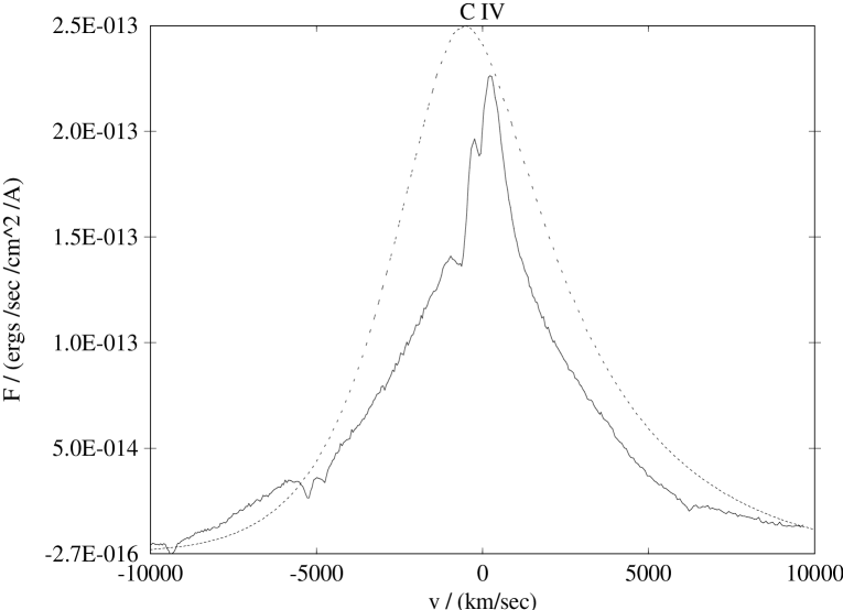
Figure L.1: Dotted line: synthetic (theoretical) C IV line profile assuming a pressure difference of 2.0 in the leading/trailing cloud edges. This calculation assumes a simple virial emission cloud model with an occulting broad line region accretion disk. Solid line: the time-averaged continuum-subtracted C IV line profile of NGC 5548, shown for comparison. Note that the observed line profile has a blueshifted absorption feature. Without this absorption feature, the peak of the line profile (which is slightly redshifted) would probably be blueshifted.

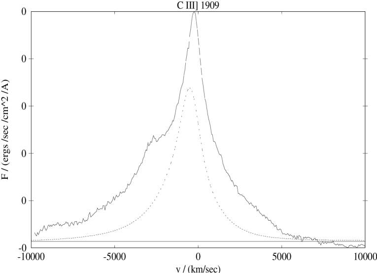
Figure L.2: Dotted line: C III] line profile for the same model as that shown in Figure L.1. Solid line: C III] profile of NGC 5548.

Figures L.1 and L.2 show the C IV and C III] line profiles for the cometary star model under the two-zone approximation assuming a face-on accretion disk and a head to tail pressure ratio parameter of 2.0. Though there are slight blue shifts of the line peaks, at first glance these synthetic profiles appear relatively innocuous.

A more careful analysis, however, reveals that the high velocity dispersion components of these synthetic line profiles are also shifted. These shifts indicate a correlation between mean line-of-sight velocity and distance from the central black hole for this model, which assumes that the clouds are in orbital motions. This correlation is revealed in the bisector shift plot (see, e.g., Kulander & Jefferies 1966) shown in

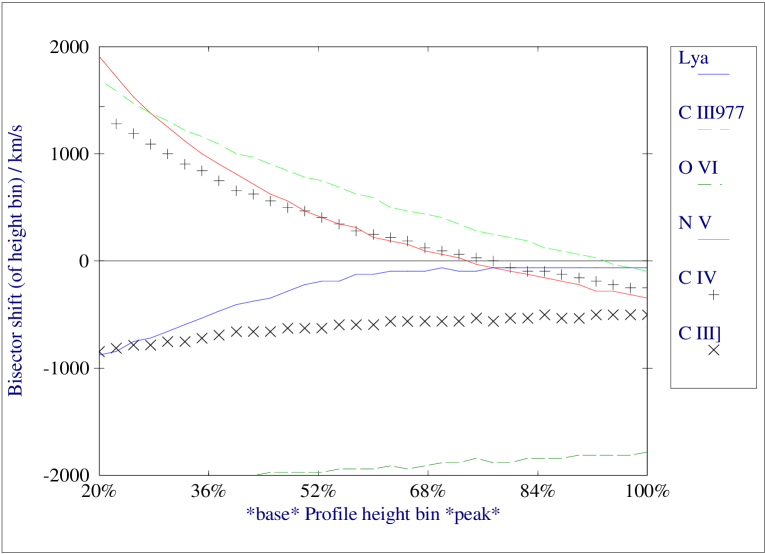
Figure L.3: Bisector shift plot for several lines. Parameters are as in Figures L.1 and L.2. Bisector shift plots show the shift of the peak of the square-shaped truncated profile verses truncation height. For this model, the peaks of the C IV and C III] lines are shifted towards the blue even though the bases are shifted in opposite directions.

Figure L.3. Note that the broader components (near the base) of the synthetic C IV line profile are shifted to the red, while the narrower components are shifted towards the blue. These shifts generally agree with empirical results (e.g., Brotherton et al. 1994). In particular, they are able to explain the apparent redshifted C IV profile base (see also Figure 4.8).

Shifts occur in the cometary star model not because of any non-zero mass flux imposed upon the model, but rather because of differences in the line luminosities between the inbound and outbound clouds. In order to understand how such differences in emissivity are possible, it is necessary to first understand how the line emissivities depend upon the ionization parameter and pressure. The ram pressure from the intercloud medium is assumed to make the ionization states of the inbound clouds lower in the inverse Strömgren region than the tail-illuminated outbound ones. The situation is illustrated in Figures L.4 and L.5.

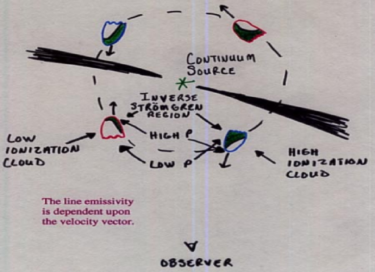
Figure L.4: Pictorial representation of clouds in the cometary star model. Clouds on the far side of the accretion disk are invisible to the observer. Clouds on the near side going towards the observer produce blueshifted line emission. Clouds on the near side going away from the observer produce redshifted line emission. Each of the four clouds shown is assumed to have the same $r$ and local continuum flux. The total line emission from lines requiring relatively low ionization is stronger for the inbound clouds than the outbound clouds. For lines in which the beaming factor does not change significantly, the resultant profile is redshifted. Conversely, lines requiring relatively high ionization in which the beaming factor does not change significantly are blueshifted.

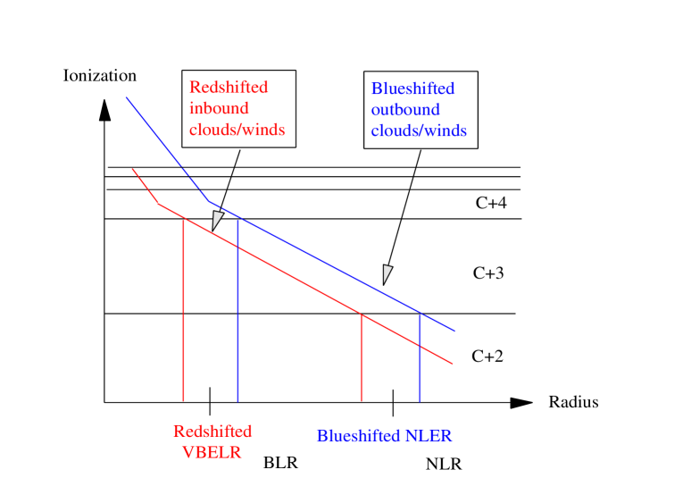
Figure L.5: Effective ionization parameter verses radius from the central continuum source for inbound clouds going towards the black hole and outbound clouds going away from the black hole. The two black horizontal lines indicate the ionization parameters where the dominant fractional ionizational abundance of carbon changes from C⁺² to C⁺³ and from C⁺³ to C⁺⁴. Here we assume $s<2,$ where $P\propto r^{-s},P$ is the mean cloud pressure, and $r$ is the radius from the central black hole. Thus the ionization decreases with radius. The (upper) diagonal blue line is the effective ionization parameter for outbound clouds as a function of radius. The (lower) diagonal red line is similar but is for inbound clouds. For C IV, there is an outermost radius (shown as the right vertical blue line) beyond which the fractional ionic abundance of C⁺³ is too low for significant emission or self-absorption to be possible. In the region denoted by the rightmost red and blue vertical lines, only the outbound clouds, which in the cometary star model have higher mean ionization parameters, should be able to emit substantial line radiation. Thus the profile bases of normal intermediate-ionization lines like C IV are redshifted, while the profile peaks are blueshifted.

Since the line emissivity from a cloud is a strong function of the ionization state, it is also a strong function of the velocity direction. The reason this velocity-dependent emission produces shifts is because of an occulting accretion disk, which is assumed to block all of the far clouds.

A unique feature of the cometary star model is that each line can have a different shift without there being any special ion-dependent cloud motions. Previous models appear to require ion-dependent cloud motions in order to explain the ion-dependent line shifts that have been observed. Such ion-dependent cloud motions plaguing previous models would appear to be physically unsatisfactory for several reasons. One of these reasons is that the line shifts do not appear to be a monotonic function of the ionization state associated with the transition (Tytler & Fan 1992). In other words, previous models have difficulty explaining “out of order” lines, like Ly$\alpha$ and C III]. In the cometary star model, the relevant variables are the gains of the line emissivities with respect to both the ionization parameter and pressure. Since Ly$\alpha$ is unusual in that it is a recombination line, it is shifted much less than the other lines. On the other hand, C III] is unusual in that it has a very negative pressure gain, and is naturally enhanced in the outbound clouds. Thus, in the cometary star model the base of this line is blueshifted much more than that of other lines without there being any special ion-dependent cloud motions.

These shifts would have a direct effect upon the velocity dependence of the variability characteristics. For the C IV line profile, which is predicted to have a redshifted base, the red-ward wing would respond more rapidly than the blue-ward wing. For the C III] profile, which has a blueshifted profile base, the situation is reversed. The blue-ward wing of this line would respond more rapidly than the red-ward wing. Previous models attempt to explain asymmetric response by invoking either outflow or inflow which would apparently predict the same red/blue response asymmetries for all lines. Thus, a good way to test the cometary star model against other models is to see whether or not the C III] line has a reversed red/blue response asymmetry.

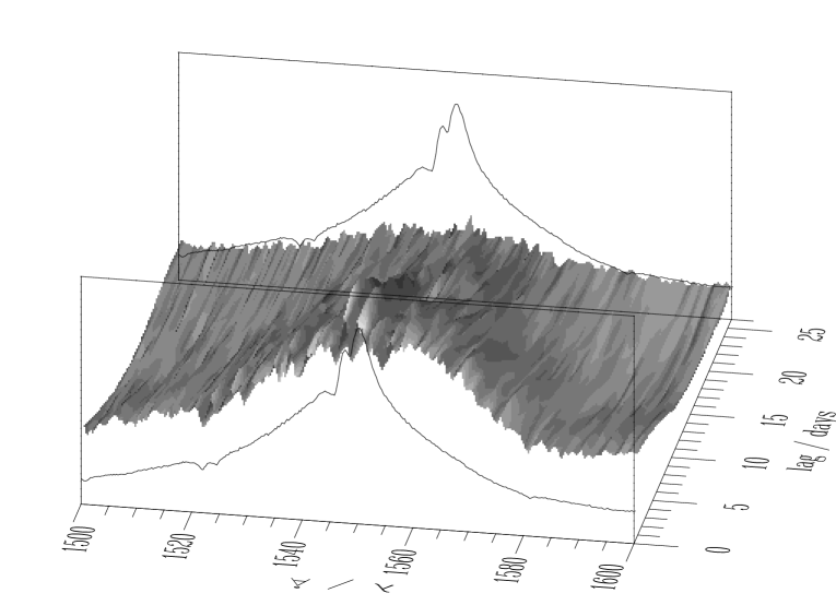
Figure L.6: The frequency-dependent cross covariance between the 1135-1180 de-redshifted continuum and the C IV spectral region.

Figure L.6 shows the cross covariance between the 1135-1180 de-redshifted continuum for the C IV spectral region of NGC 5548 using the HST variability campaign data (Korista et al. 1995).

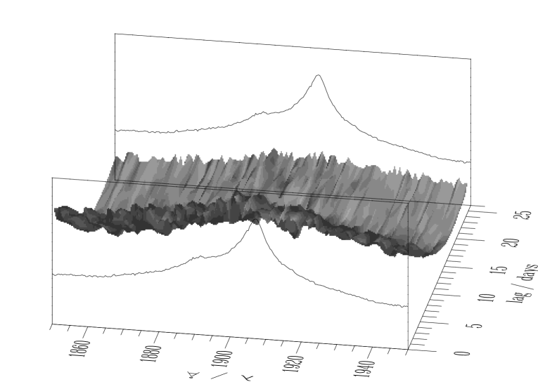
Figure L.7: The frequency-dependent cross covariance between the 1135-1180 de-redshifted continuum and the C III]/Si III]/Al III spectral line region.

Figure L.7 shows the equivalent C III]/Si III]/Al III spectral line region. At lags of less than a few days, there is significant response due to the underlying continuum, which was not subtracted. Superimposed upon this response is an additional response that is proportional to the absolute line flux presumably emitted from the clouds. At a lag of 25 days, the response is nearly symmetric for each wing. At lags below 5 days, however, the blue wing of C IV appears to have a slightly stronger response amplitude than the red wing of C IV. Though it is difficult to determine with certainty, Figure L.6 appears to indicate that C III] indeed exhibits the reverse behavior. These effects are small and the analysis provided here is very crude. Nevertheless, similar results have been found in the more complete studies of the NGC 5548 data. While it would be a straightforward task to concoct models with ion-dependent cloud motions to explain just these particular observations, perhaps the simplest interpretation is that the broad components of several lines are often shifted and that the red-ward C IV and blue-ward C III] emissions are indeed closer on the average to the central black hole. As

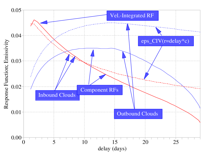
Figure L.8: Solid lines: response functions for a simplified cometary star model. Dotted lines: approximated C IV line emissivity. The head/tail pressure ratio was assumed to be 2.0 in these calculations.

Figure L.8 shows, this is precisely what was naturally predicted by the cometary star model.

Surveys indicate that the peaks of C III] are shifted to the blue more than the peaks of C IV. NGC 5548 is no exception to this trend. Though the line shifts shown on the previous page match this ordering, many of the models I calculated that fared better regarding line ratios did not match this ordering.

One possible explanation for this shortcoming of some of the models is that self-absorption was not accounted for in my simulations. Self-absorption from clouds along the line of sight that are farther away from the central black hole than the other clouds emitting a line should be detectable because of the required high geometrical covering factors and the high signal to noise ratios near the line peaks. As Figure L.5 shows, for $s<2$ models there is an outermost radius beyond which the fractional ionic abundance is too low for significant self-absorption to be possible in most lines. For this reason, the self-absorption “components” of most line peaks should be blueshifted. Because the self-absorbing clouds must be along the line of sight, they should appear to have non-causal local response functions (zero delay, yet low velocity dispersions in a spherically symmetric orbital system).

Both of these features appear to exist in the lines of the high-quality NGC 5548 HST data (including the C IV 1548.20/1550.77 doublet resolved in the plot on the previous page). Note that this self-absorption results in an effective countering redshift of the profile peak.

This behavior, however, does not apply to all lines. In particular, C III] $\lambda 1909$ has such a low absorption oscillator strength $(10^{-6}$ that of C IV) that it should be immune from such self-absorption. Therefore, its profile shape should not be influenced by self-absorption and the blueshift of its observed profile peak should be higher than that of most other lines in AGNs that have high covering factors. Hopefully, future modeling efforts will quantitatively test this as well as other apparent predictions of the cometary star model.   Pages on which citations occur are listed as boldfaced numbers.

• Adams, F. & Fatuzzo, M. 1996, ApJ, 464, 256  192, 204

  Alexander, T. & Netzer, H. 1994, MNRAS, 270, 78 (AN94)  9, 33–35, 55, 176, 186–188, 228

  Alexander, T. & Netzer, H. 1997, MNRAS, 284, 967 (AN97)  33, 75, 80, 131, 176, 186–188, 190, 198–200, 228

  Allen, A. J. 1984, MNRAS, 210, 147  13

  Alloin, D., Clavel, J., Peterson, B. M., Reichert, G. A., & Stirpe, G. M. 1994, in Frontiers of Space and Ground-based Astronomy, ed. W. Wamsteker, M. S. Longair, & Y. Kondo (Dordrecht: Kluwer), 423  17

  Antona, F. D. & Ergma, E. 1993, A&A, 269, 230  31, 32, 236

  Arav, N., Barlow, T. A., Laor, A., & Blandford, R. D., 1997, MNRAS, 288, 1015  35, 313, 317

  Arav, N., Barlow, T. A., Laor, A., Sargent, W. L. W. & Blandford, R. D., 1998, MNRAS, 297, 990  35, 313, 317

  Arav, N., Li, Z., & Begelman, M. C. 1994, ApJ, 432, 62  311

  Aretxaga, I., Cid Fernandes, R., & Terlevich, R. J. 1997, MNRAS, 286, 271  9

  Augarde, R. & Lequeux, J. 1985, A&A, 147, 273  204

  Bahcall, J. N. & Soniera, R. M. 1984, ApJS, 55, 67  207, 213, 214

  Bahcall, J. N., Wolf, R. A., 1977, ApJ, 216, 883  189

  Baldwin, J. A. 1977, ApJ, 214, 679  30, 33, 53, 71, 321

  Banit, M. & Shaham, J. 1992, ApJ, 388, 19L  28

  Barlow, T. A. 1994, PASP, 106, 548  304

  Barlow, T. A. 1995, BAAS, 186, 4209  310

  Basko, M. M. & Sunyaev, R. A. 1973, Ap&SS, 23, 117  28

  Beard, D. 1981, ApJ, 245, 743  226

  Beltrametti, M. 1981, ApJ, 250, 18  13

  Binney, J. & Tremaine, S. 1987, Galactic Dynamics (Princeton: Princeton University Press)  62, 212, 215, 297

  Blandford, R. D. & McKee, C. F. 1982, ApJ, 255, 419  38, 40, 231, 233, 237, 242, 243, 249, 257, 261, 262, 264, 286, 292

  Bodenheimer, P., Tohline, J. E., & Black, D. C. 1980, ApJ, 242, 209  204

  Boller, T., Brandt, W., & Fink, H. 1996, A&A, 305, 53  164

  Brandl, B., Sams, B. J., Bertoldi, F., Eckart, A., Genzel et al. 1996, ApJ, 466, 254  194, 196, 202, 204–206

  Brighenti, F., & D’ercole, A. 1995, MNRAS, 273, 443  226

  Brotherton, M. S., Wills, B. J., Steidel, C. C., Sargent, W. L. W. 1994, ApJ, 423, 131  323

  Campbell, B., et al. 1992, AJ, 104, 1721  202

  Cassidy, I., & Raine, D. J., 1993, MNRAS, 260, 395  9

  Collin-Souffrin, S. 1987, A&A, 179, 60  9, 18, 80

  Cooke, B. A., Fabian, A. C. & Pringle, J. E. 1978, Nature, 273, 645  226

  Crenshaw et al. 1996, ApJ, 470, 322  315

  de Jong, R. S. 1996, A&A, 313, 377  203, 215

  Doane, J. S. & Mathews, W. G. 1993, ApJ, 419, 573  204

  Done, C. & Krolik, J. H. 1996, ApJ, 463, 144  3, 33, 82, 84, 86, 87, 154, 174

  Doyon, R., Joseph, R. D., & Wright, G. S. 1994, ApJ, 421, 101  204

  Dumont, A., Collin-Souffrin, S., & Nazarova, L. 1998, A&A, 331, 11  80, 101, 102

  Dwek, E. 1998, ApJ, 501, 643  214

  Eckart, A., Genzel, R., Hofmann, R., Sams, B. J., Tacconi-Garman, L. E., 1993, ApJ, 407, L77  64

  Edelson, R., et al. 1993, BAAS, 183, 3006  302

  Edelson, R., et al. 1996, ApJ, 470, 364  316

  Edmunds, M. G. & Phillipps, S. 1989, MNRAS, 241, 9  203

  Edwards, A. C. 1980, MNRAS 190, 757  9, 28, 29, 31, 54

  Eilek, J. A. & Caroff, L. J. 1979, ApJ, 233, 463  13

  Emmering, R. T., Blandford, R. D., & Shlosman, I. 1992, ApJ, 385, 460  9, 13

  Eracleous, M. & Halpern, J. 1994, ApJS, 90, 1  9, 18–22

  Eracleous, M. & Halpern, J. 1993, ApJ, 409, 584  9, 18–22

  Evans, C. R. & Kochanek, C. S. 1989, ApJ, 346, L13  27

  Fall, S. M. & Efstathiou, G. 1980, MNRAS, 193, 189  7

  Fath, E. 1909 Lick Observatory Bulletin 5, 71  2, 4

  Ferland, G. J., Peterson, B. M., Horne, K., Welsh, W. F., & Nahar, S. N. 1992, ApJ, 387, 95  10

  Frank, A., Noriega-Crespo, A. Balick, B. 1992, AJ, 104, 841  28

  Friel, E. D. & Janes, K. A. 1993, A&A, 267, 75  220

  Garmany, C. D., Conti, P. S., & Chiosi, C. 1982, ApJ, 263, 777  203, 211, 213

  Gaskell, C. M. 1997, BAAS, 191, 2506  20

  Goad, M. R., O’Brien, P. T., & Gondhalekar, P. M. 1993, MNRAS, 263, 149  58, 262, 264

  González, R. A. & Graham, J. R. 1996, ApJ, 460, 651  212

  Hamann, F. & Ferland, G. 1992, ApJ, 391, L53  225

  Hamann, F., Korista, K. T., & Morris, S. L. 1993, ApJ, 415, 541  310

  Hameury, J., King, A., Lasota, J., & Raison, F. 1993, A&A, 277, 81  28, 32

  Harpaz, A., & Rappaport, S. 1995, A&A, 294L, 49  28, 31, 236

  Harpaz, A., & Rappaport, S. 1991, ApJ, 383, 739  28, 31, 236

  Hartwick, F. D. A. 1970, ApJ, 161, 845  203

  Hills, J. G. 1975, Nature, 254, 295  27

  Ho, L. C. 1996, PASP, 108, 637  2

  Horne, K., Welsh, W. F., & Peterson, B. M. 1991, Ap.J., 367, L5-L8  19, 310

  Hubeny, I. 1994, in Theory of Accretion Disks–2, ed. W. J. Duschl, J. Frank, & F. Meyer (Dordrecht: Kluwer Academic)  25

  Hubeny, I. & Hubeny, V. 1997, ApJ, 484, L37  181

  Humphreys, R. M. 1978, ApJS, 38, 309  203

  Humphreys, R. M. & McElroy, D. B. 1984, ApJ, 284, 565  203

  Hunter, D. A., et al. 1996, ApJ, 459, L27  194, 195, 205

  Hutchings, J. B., Cowley, A. P., Crampton, D., van Paradijs, J., & White, N. E. 1979, Ap. J., 229, 1079  25

  Iwamoto, K., Mazzali, P. A., Nomoto, K., Umeda, H. et al. 1998, Nature, 395, 672  225

  Kallman, T. R. 1995, ApJ, 455, 603  58, 251

  Kallman, T. R. & Krolik, J. H. 1986, ApJ, 308, 805  9, 10

  Kallman, T. R., Wilkes, B. J., Krolik, J. H., & Green, R. 1993, ApJ, 403, 45  13, 257

  Kaspi, S., et al. 1996, ApJ, 471, L75  117, 175, 187

  Kazanas, D. 1989, ApJ, 347, 74  2, 9, 32–34, 47, 50–52, 54, 59, 68, 77, 117, 162, 172–174, 228, 244, 320

  Kent, S. M. 1986, AJ, 91, 1301  213

  Kinney, A. L., Rivolo, A. R., & Koratkar, A. P. 1990, ApJ, 357, 338  33, 41

  Koratkar et al. 1996, ApJ, 470, 378  310, 316

  Korista, K. T., et al. 1995, ApJS, 97, 285  4, 17, 33, 71, 76, 310, 323, 328

  Krinsky, I. & Puetter, R. 1992, ApJ, 394, 472  13, 53, 236

  Krolik, J. H. 1988, ApJ, 325, 148  13

  Krolik, J. H. & Done, C. 1995, ApJ, 440, 166  80, 82, 83, 86

  Krolik, J. H., Horne, K., Kallman, T. R., Malkan, M. A., & Edelson, R. A. 1991, ApJ, 371, 541  19, 53, 73, 100, 101, 252, 262, 283, 287, 292

  Krolik, J. H., McKee, C. F., & Tarter, C. B. 1981, ApJ, 249, 422 (KMT)  9, 11, 47, 52, 234, 236

  Kuijken, K. & Gilmore, G. 1991, ApJ, 367, L9  206, 207, 212–214

  Kuijken, K. & Gilmore, G. 1989a, MNRAS, 239, 571  206, 207, 213

  Kuijken, K. & Gilmore, G. 1989b, MNRAS, 239, 605  212, 214

  Kulander, J. & Jefferies, J. 1966, ApJ, 146, 194  323

  Kulkarni, S. R. & Narayan, R. 1988, ApJ, 335, 755  28

  Kwan, J. Y. & Krolik, J. H. 1979, ApJ, 233, L91  24, 55

  Kwan, J. Y. & Krolik, J. H. 1981, ApJ, 250, 478  24

  Kwan, J., Cheng, F. Z., & Zongwei, L. 1992, ApJ, 393, 87  32

  Lacy, J. H., Townes, C. H., & Hollenbach, D. J. 1982, ApJ, 262, 120  26

  Langer, N. & Maeder, A. 1995, A&A, 295, 685  203

  Laor, A., Bahcall, J. N., Jannuzi, B. T., Schneider, D. P., & Green, R. F., et al. 1994, ApJ, 420, 110  10, 77, 258

  Larson, R. B. 1982, MNRAS, 200, 159  204

  Lauer, T. R., Ajhar, E. A., Byun, Y., Dressler, A., Faber, S. M. et al. 1995, AJ, 110, 2622  62, 64, 68, 73

  London, R. A. & Flannery, B. P. 1982, ApJ, 258, 260  28

  London, R. A., McCray, R., & Auer, L. H. 1981, ApJ, 243, 970  28, 30

  MacDonald, J., Stanev, T., & Biermann, P. L. 1991, 378, 30  188

  Malkan, M. A., Gorjian, V., & Tam, R., 1998, ApJS, 117, 25  64

  Malumuth, E. M. & Heap, S. R. 1994, AJ, 107, 1054  192, 202, 204

  Maoz, D. 1992, in Physics of Active Galactic Nuclei, ed. W. J. Dushl & S. J. Wagner (Berlin: Springer-Verlag), 214  41, 287

  Maoz, D., Netzer, H., Mazeh, T., Beck, S., & Almozino, E., et al. 1991, ApJ, 367, 493  12

  Marshall, F. E., Netzer, H., Arnaud, K. A., Boldt, E. A., Holt, S. S. et al. 1993, ApJ, 405, 168  216, 217, 221, 223, 224

  Massey, P., Johnson, K. E., & Degioia-Eastwood, K. 1995, ApJ, 454, 151  193, 194

  Mathews, W. G. & Blumenthal, G. R. 1977, ApJ, 214, 10  13

  Mathews, W. G. & Ferland, G. J. 1987, ApJ, 323, 456  13, 227

  Mazzali, P. & Chugai, N. 1995, A&A, 303, 118  225

  McClure, R. D. & ven den Bergh, S. 1968, AJ, 73, 313  203

  McCray, R. A. 1979, in Active Galactic Nuclei (Cambridge: Cambridge University Press), ed. C. R. Hazard & S. Mitton  9, 11, 30

  Mestel, L. 1965, QJRAS, 6, 161  7, 212

  Mestel, L. 1963, MNRAS, 126, 553  7, 212

  Mihalas, D. & Binney, J. 1978, Galactic Astronomy (New York: Freeman)  215

  Miller, G. E. & Scalo, J. M. 1979, ApJS, 41, 513  210, 212, 213

  Morton, D. C. 1991, ApJS, 77, 119  323

  Mulchaey, J. S., Davis, D. S., Mushotzky, R. F., & Burstein, D. 1996, ApJ, 456, 80  214

  Murphy, B. W., Cohn, H. N., & Durisen, R. H. 1991, ApJ, 370, 60  26, 61, 68, 186

  Murray, N., Chiang, J., Grossman, S. A., & Voit, G. M. 1995, ApJ, 451, 498  9, 21–23, 301, 311, 312, 317

  Netzer, H. 1990, in Active Galactic Nuclei (Berlin: Springer-Verlag), ed. T. Courvoisier & M. Mayor, 57  232

  Norman, C. & Scoville, N. 1988, ApJ, 332, 124  9, 32, 54, 172

  Osterbrock, D. E. 1993, ApJ, 404, 551  20

  Padoan, P., Nordlund, A., & Jones, B. J. T. 1997, MNRAS, 288, 145  191, 192, 202–204

  Panagia, N. & Tosi, M. 1981, A&A, 96, 306  220

  Peebles, P. J. 1993, Principles of Physical Cosmology (Princeton: Princeton University Press)  214

  Peimbert, M. 1992, in The Astronomy and Astrophysics Encyclopedia, ed. S. P. Maran (New York: Van Nostrand Reinhold), 356  219, 220

  Penston, M. V. 1985, MNRAS, 212, 939  32, 54

  Penston, M. V., 1988, MNRAS, 233, 601  32, 54

  Peterson, B. 1994, in Reverberation Mapping of the Broad-Line Region in Active Galactic Nuclei, ed. P. M. Gondhalekar, K. Horne, and B. M. Peterson, 1  258

  Phillipps, S., Edmunds, M. G., & Davies, J. I. 1990, MNRAS, 244, 168  203

  Pijpers, F. P. & Wanders, I. 1994, MNRAS, 271, 183  86

  Podsiadlowski, P. 1991, Nature, 350, 136  28, 32

  Pogge, R. W., Peterson, B. M. 1992, AJ, 103, 1084  287, 292

  Pringle, J. E. 1981, ARA&A, 19, 137  16, 226

  Raine, D. J. & Smith, A. 1981, MNRAS, 197, 339  9, 10

  Rees, M. J. 1982, in The Galactic Center, ed. G. Riegler & R. D. Blandford (New York: AIP), 166  26

  Rees, M. J. 1987, MNRAS, 228, 47  236

  Rees, M. J. 1988, Nature, 333, 523  26

  Rees, M. J. 1990, Science, 247, 817  27, 28

  Rees, M. J., Netzer, H., & Ferland, G. J. 1989, ApJ, 347, 640  53, 97, 105, 107, 232, 234

  Rieke, G. H., Lebofsky, M. J., Thompson, R. I., Low, F. J., & Tokunaga, A. T. 1980, ApJ, 238, 24  204

  Rix, H. & Zaritsky, D. 1995, ApJ, 447, 82  212

  Roos, N. 1992, ApJ, 385, 108  9, 26–28

  Salpeter, E. E. 1955, ApJ, 121, 161  181, 182, 191, 210

  Sanders, R. H., & van Oosterom, W. 1984, A&A, 131, 267  26

  Scalo, J. M. 1986, FCPh, 11, 1  193, 210, 212, 213

  Schaaf, R. & Schmutzler, T. 1992, in Physics of Active Galactic Nuclei, ed. W. J. Dushl & S. J. Wagner (Berlin: Springer-Verlag), 230  236

  Schaerer, D. & de Koter, A. 1997, A&A, 322, 598-614  180

  Schaerer, D., Meynet, G., Maeder, A., & Schaller, G. 1993, A&AS, 102, 339  203

  Schaller, G., Schaerer D., Mynet G., & Maeder A. 1992, A&AS, 96, 269  184, 207

  Scoville, N. & Norman, C. 1988, ApJ, 332, 163, 1988  32, 48

  Scoville, N. & Norman, C. 1995, ApJ, 451, 510  311, 312

  Sellwood, J. A. 1985, MNRAS, 217, 127  212

  Shakura, N. I. & Sunyaev, R. A. 1973, A&A, 24, 337  16, 18, 19, 21

  Sparke, L. S. 1993, ApJ, 404, 570  254

  Tavani, M. & London, R. 1993, ApJ, 410, 281  28, 30

  Taylor, J. A. 1994, in Reverberation Mapping of the Broad-Line Region in Active Galactic Nuclei (San Francisco: ASP), ed. P. M. Gondhalekar, K. Horne, & B. M. Peterson, 341  27, 30, 53, 232, 236, 244, 253, 320

  Taylor, J. A. 1996, ApJ, 470, 269  14, 58, 273

  Taylor, J. A. 1998, ApJ, 497, L81  217

  Taylor, J. A. & Kazanas, D. 1992, in Testing the AGN paradigm, ed. S. S. Holt, S. G. Neff, & C. M. Urry, 560  245

  Toomre, A. 1974, in Highlights of Astronomy, ed. G. Contopoulos (Dordrecht: Reidel), 457  212

  Tout, C. A., Eggelton, P. P., Fabian, A. C., & Pringle, J. E. 1989, MNRAS, 238, 427  28, 31, 32, 54, 190

  Tremaine, S., Richstone, D. O., Byun, Y., Dressler, A. & Faber, et al. 1994, AJ, 107, 634  62, 63, 68, 212

  Tsujimoto, T., Nomoto, K., Yoshii, Y., Hashimoto, M., Yanagida, S. et al. 1995, MNRAS, 277, 945  224

  Turnshek et al. 1994, ApJ, 428, 93  310

  Tytler, D. & Fan, X. M. 1992, ApJS, 79, 1  328

  Ulrich, M. & Horne, K. 1996, MNRAS, 283, 748  310

  van Albada, T. S., Bahcall, J. N., Begeman, K., & Sanscisi, R. 1985, ApJ, 295, 305  204

  Voit, G. M. & Shull, J. M. 1988, ApJ, 331, 197  28, 30, 54

  Voit, G. M., Shull, J. M., & Begelman, M. C. 1987, ApJ, 316, 573  304

  Wanders, I., Goad, M. R., Korista, K. T., Peterson, B. M., Horne, K. et al. 1995, ApJ, 453, L87  82, 84, 86, 87, 154, 174

  Weisheit, J. C., Shields, G. A., & Tarter, C. B. 1981, ApJ, 245, 406  24

  Weymann, R. 1995, in QSO Absorption Lines, ed., G. Meylan (Berlin: Springer-Verlag), 213  311

  Weymann, R. 1996, preprint  314

  Wielen, R. 1977, A&A, 60, 263  212

  Wolfe, A. M. 1974, ApJ, 188, 243  9, 11, 234

  Worthey, G. 1994, ApJS, 95, 107  214

  Zheng, W., Kriss, G. A., Telfer, R. C., Grimes, J. P. & Davidsen, A. F. 1997, ApJ, 475, 469  78, 180

  Zombeck, M. 1990, Handbook of Astronomy and Astrophysics, Second Edition, (Cabridge, UK: Cambridge University Press)  69