Axisymmetric, 3-Integral Models of Galaxies: A Massive Black Hole in NGC 3379

Abstract

We fit axisymmetric 3-integral dynamical models to NGC 3379 using the line-of-sight velocity distribution obtained from HST/FOS spectra of the galaxy center and ground-based long-slit spectroscopy along four position angles, with the light distribution constrained by WFPC2 and ground-based images. We have fitted models with inclinations from 29° (intrinsic galaxy type E5) to 90° (intrinsic E1) and black hole masses from 0 to $10^{9}M_{\odot}$.

The best-fit black hole masses range from $6\times 10^{7}-2\times 10^{8}M_{\odot}$, depending on inclination. The preferred inclination is 90° (edge-on); however, the constraints on allowed inclination are not very strong due to our assumption of constant M/L_V. The velocity ellipsoid of the best model is not consistent with either isotropy or a two-integral distribution function. Along the major axis, the velocity ellipsoid becomes tangential at the innermost bin, radial in the mid-range radii, and tangential again at the outermost bins. The rotation rises quickly at small radii due to the presence of the black hole. For the acceptable models, the radial to tangential (($\sigma_{\theta}^{2}+\sigma_{\phi}^{2})/2)$ dispersion in the mid-range radii ranges from $1.1<\sigma_{r}/\sigma_{t}<1.7$, with the smaller black holes requiring larger radial anisotropy. Compared with these 3-integral models, 2-integral isotropic models overestimate the black hole mass since they cannot provide adequate radial motion. However, the models presented in this paper still contain restrictive assumptions—namely assumptions of constant M/L_V and spheroidal symmetry—requiring yet more models to study black hole properties in complete generality.

1. Introduction

The dynamical state and mass distribution in the central regions of elliptical galaxies provide clues to the formation and evolutionary histories of these galaxies (see Merritt 1999 for a review). Consequently, the existence of central black holes has been the target of intense scrutiny (see Kormendy & Richstone 1995 for a review). In this paper, we study the elliptical galaxy NGC 3379 using both Hubble Space Telescope and ground-based photometric and kinematic data in order to understand its central dynamics.

At ground-based resolution NGC 3379 is a prototypical elliptical (E1) galaxy with M${}_{V}=-20.6$ (Faber et al. 1997) at a distance of 10.4 Mpc (Ajhar et al. 1997). Lauer et al. (1995) classify it as a “core” galaxy—a galaxy that has a break in the surface brightness profile but still maintains a rising profile into the smallest measured radius. Faber et al. (1997) hypothesize that core galaxies are associated with massive black holes. However, few core galaxies have strong black hole detections: M87 (Harms et al. 1994), M84 (Bower et al. 1998), and N4261 (Ferrarese et al. 1996). These detections result from gas dynamics, not stellar dynamics. Stellar dynamical evidence for central black holes in core galaxies is difficult to obtain since (1) core galaxies have low surface brightnesses, making kinematic observations difficult, (2) the lack of rotation complicates the dynamical modeling since velocity anisotropies potentially govern the dynamical support, and (3) stars near the center travel out to the core radius so their contribution to the central velocity profile is de-weighted (Kormendy 1992). NGC 3379 was chosen for this study because of its relatively high central surface brightness among core galaxies, and because of its otherwise normal morphological and dynamical structure.

The proximity, brightness, and normalcy of NGC 3379 make it the object of many ground-based photometric (de Vaucouleurs & Capaccioli 1979, Lauer 1985, Capaccioli et al. 1987, Capaccioli et al. 1991) and kinematic (Kormendy 1997, Kormendy 1985, van der Marel et al. 1990, Bender et al. 1994, Statler 1994, Statler & Smecker-Hane 1999) studies. However, previous models for NGC 3379 have yielded inconsistent results. Assuming that the departure of the light profile from the $R^{1/4}$ law signifies the existence of a stellar disk, Capaccioli et al. (1991) find that the most likely model is nearly face-on with an inclination of 31° (intrinsic E5 galaxy). Their conclusion was that NGC 3379 and NGC 3115 have the same intrinsic shape but are seen from different viewing angles. In their model for NGC 3379 the central region is nearly oblate, but at about $r=0.5r_{e}$ ($r_{e}=35$″) the model becomes triaxial. No dynamical information was used in this model. A major uncertainty is that slight departures from a $R^{1/4}$ law, on which their model is based, may be due to tidal effects (Kormendy 1977) instead of a disk. Furthermore, there is no reason to expect galaxies to follow a $R^{1/4}$ law exactly.

Kinematic information is required to determine unambiguously the inclination of a spheroidal system. Van der Marel et al. (1990), using the ground-based velocity data of Davies & Birkinshaw (1988) and Franx et al. (1989), conclude that the inclination of NGC 3379 is 60°; however the two datasets are not consistent and give slightly different velocity anisotropy parameters. Van der Marel et al. used 2-integral flattened models with a parametrized form for the anisotropy. No goodness-of-fit criteria were given, and thus we are not able to compare their results with those of others. Statler (1994), using Bayesian statistics on the same datasets, prefers models that have inclination greater than 45°. Statler rejects Capaccioli’s conclusion that the galaxy is flattened and triaxial at the 98% confidence level, but his results could accommodate those of van der Marel et al. Statler uses only the mean velocity measured along four position angles; the radial variation in the velocity or the dispersion are not considered. Furthermore, Statler uses data only outside 15″. However, Statler has obtained new, high S/N data (Statler & Smecker-Hane 1999), which he will present in a future paper.

The studies above use low S/N, sparse kinematic data, or no kinematic data at all. In this paper, we report results from observations of the full line-of-sight velocity distribution (LOSVD) at various position angles from high S/N ground-based data and data from HST. The data are fit to axisymmetric, three-integral orbit-based models. Richstone et al. (1999) describe the modeling technique in a companion paper. We exploit the full LOSVDs directly in the modeling. Alternatively, we could use the moments of the LOSVDs; however, the full shape of the LOSVD contains important information on the underlying dynamics, and it is desirable to incorporate the full LOSVD when the spectra have sufficient signal-to-noise to determine this reliably. In fact, our result for NGC 3379 critically depends on the shape of the central LOSVD. Cretton et al. (1999) and van der Marel et al. (1998) present a very similar modeling technique, where the only difference from ours is that we fit the full LOSVD as opposed to their moment fitting procedure. There are other programs that also use the higher moments of the LOSVD as constraints (Dejonghe, 1987; Gerhard 1993; Rix et al. 1997). Obtaining the full LOSVD at many position angles is the maximum obtainable kinematic information and has now become routine (e.g. Bender et al. 1994, Carollo et al. 1995, Gebhardt & Richstone 1999).

In §2, we describe the photometric and kinematic data for NGC 3379. In §3, we describe the models and present results in §4. Discussion is given in §5.

2. Data

2.1. Photometry: HST and Ground-Based Imaging

We obtained Hubble Space Telescope (HST) observations of NGC 3379, consisting of four 500s F555W ($V$-band) and four 400s F814W ($I$-band) WFPC2 images, on 1994 November 19. Centering the galaxy in the high-resolution PC1 camera (0.0455″ pixel^-1) provided a total signal in the central pixel of $\sim 2\times 10^{4}e^{-}$ in both $V$ and $I$. We deconvolved the summed images with 40 Lucy-Richardson iterations. The surface brightness, ellipticity, and position angle of the major axis were obtained using the same procedure as in Lauer et al. (1995) and are presented in Table 1.

Visual surface brightness and luminosity density for NGC 3379. The solid circles are the data from HST and the solid triangles are the data from Peletier et al. (1990), which have been adjusted to match with the HST data assuming constant color. The solid line in the left panel represents a smoothing spline (Gebhardt et al. 1996) of the surface brightness data. The inferred luminosity density is given for three different inclinations; from bottom to top the lines represent the densities at 90° (intrinsic E1), 31° (E4), and 27° (E6).

The HST profile reaches only about 12″ from the center and must be extended to larger radii using ground-based photometry. Peletier et al. (1990) have obtained ground-based $UBR$ photometry for NGC 3379 over the radius range 4″–170″, and Capaccioli et al. (1990) have $B$ photometry out to 500″; we must therefore estimate the transformations to $V$ and $I$ using the overlap region with the HST data. The data from Peletier et al. and Capaccioli et al. agree well, and since Peletier et al. provide several colors, we use their results. The colors in the overlap region, based on the average differences there, are $B-V=-0.58$ and $R-I=-0.94$. We have ignored possible variations in the colors as a function of radius. Using these colors, we combine the HST and ground-based data to provide the full profile. The left panel in Fig. 1 shows the surface brightness profile in $V$ along the major axis from 0.02″–170″. The three panels in Fig. 2 show the ellipticity, the position angle of the major axis (measured from north through east), and the color $V-I$ as functions of radius along the major axis. The random uncertainties can be estimated from the local scatter.

The dynamical modeling described below assumes axisymmetry. We must therefore determine the best axisymmetric density distribution consistent with the observed surface brightness distribution. Strictly speaking, there is none, because, as shown in Figure 2, there are abrupt changes in the ellipticity and position angle at radii less than 1″ and larger than 100″. PA changes in particular are normally attributed to variation in the axis ratios with radius in a triaxial distribution, or to real three-dimensional twists in locally axisymmetric objects in which surfaces of constant density, while axisymmetric, are not co-axial.

Ellipticity, position angle and $V-I$ color as a function of radius along the major axis for NGC 3379. The solid circles are the data from HST, and the solid triangles are data from Peletier et al. (1990). The ground-based $V-I$ is estimated from $B-R$.

However, for several reasons we believe that, at radii less than 100″, an axisymmetric model will suffice for our purposes. First, in the middle range of radii, $1\arcsec<r<100\arcsec$, the ellipticity and PA are fairly constant at 0.1 and 72 $\pm$ 5°. Second, in the central region there is a dust ring with radius 1″ (discussed below and seen in Fig. 5). The absorption by the dust ring – 1% of the galaxy surface brightness – is enough to affect estimates of both the ellipticity and the position angle. Furthermore, the shallow central slope (dlog $\Sigma$/dlog $R=-0.2$) of the inner profile and the small ellipticity ($\sim 0.1$) render the position angle at small radii ($R<1\arcsec$) highly uncertain. Even if the PA gradient seen in Fig 2 is real and well determined, the amount of light, and therefore the gravitational impact, of the associated departure from axisymmetry is small. Finally, at large radii, departures from axisymmetry have little impact on the central gravitational field.

The data thus suggest that NGC 3379 can be reasonably well represented by a spheroid of constant ellipticity. The deprojection of the surface brightness is then unique for a given inclination. The deprojection is based on a non-parametric estimate of the density using smoothing splines (Gebhardt et al. 1996). The right panel of Fig. 1 plots the luminosity density for three different inclinations (90° is edge-on). For different inclinations, and hence different flattenings, the luminosity density scales as the ratio of the apparent to the true axis ratio.

We did not examine models in which the galaxy is assumed to be axisymmetric but not spheroidal (i.e., with varying ellipticity), in part because in this case the deprojection is not unique. Romanowsky & Kochanek (1997) determine the uncertainties in the deprojection of an axisymmetric system for various inclinations, and the uncertainties can be quite large for low inclinations (close to face-on). We could test the effect of our spheroidal assumption by modeling the most extreme situation: a galaxy which is seen nearly face-on and containing an embedded disk (similar to the suggestion of Capaccioli et al. 1991). The most likely effect is to change to inclination and M/L_V constraints, and relaxing the spheroidal assumption should have little effect on the measured black hole mass. This issue, however, will not be addressed here.

2.2. HST FOS Spectroscopy

NGC 3379 was observed on 1995, January 23 – 27 with the 0.21″ square aperture (“0.25-PAIR”) of the FOS. The spectrum was taken in two visits; the total integration time was 215.5 minutes.

The wavelength range, 4566–6815 Å, includes the Mg I b lines at $\lambda\simeq 5175$ Å and the Na I D lines at $\lambda\simeq 5892$ Å. The spectrum was electronically quarter-stepped, giving 2064 1/4-diode pixels. The reciprocal dispersion was 1.09 Å pixel^-1. The instrumental velocity dispersion was measured to be $\sigma_{\rm instr}=$FWHM/2.35$=1.76\pm 0.03$ pixels = $101\pm 2$ $\rm{km}~{}\rm s^{-1}$ (internal error). This width is intrinsic to the instrument and is not strongly affected by how the aperture is illuminated (Keyes et al. 1995). We therefore make no aperture illumination corrections to the measured velocity dispersion.

Flat fielding and correction for geomagnetically induced motions (GIM) were done as in Kormendy et al. (1996). The flat-field image was taken with the same 0.25-PAIR aperture used for NGC 3379. The galaxy exposure was divided into 3 and 4 subintegrations for the two visits. Because GIM shifts between subintegrations are small, unlike the large shifts between galaxy exposures and the flat field, we first averaged all the exposures and used cross-correlation to determine the shift between this average and the flat field. The measured shift was 2.27 pixel. Each subintegration was multiplied by the flat-field frame shifted by the above amount. One dead diode was corrected by dividing the affected pixel intensities by 0.8. Then GIM shifts between subintegrations were determined; most shifts were $<0.5$ pixels, with the largest being 0.8 pixels. Each subintegration was then shifted to agree with the subintegration taken closest in time to the comparison spectrum exposure. Finally, the spectra were added, weighted by the exposure times.

2.2.1 Extracting the LOSVD

Obtaining the internal kinematic information requires a deconvolution of the observed galaxy spectrum with a representative set of template stellar spectra. We deconvolve the spectrum using a maximum-penalized likelihood (MPL) estimate that obtains a non-parametric line-of-sight velocity distribution (LOSVD). The fitting technique proceeds as follows: we choose an initial velocity profile in bins. We convolve this profile with a weighted-averaged template (discussed below) and calculate the residuals to the galaxy spectrum. The program varies the velocity profile parameters—bin heights—and the template weights to provide the best match to the galaxy spectrum. The MPL technique is similar to that used in Saha & Williams (1994), and Merritt (1997). However, in constrast to these authors we simultaneously fit the velocity profile and template weights. We impose smoothness on the LOSVD by the addition to the $\chi^{2}$ of a penalty function, which is the integrated squared second derivative (details are in Merritt 1997 and Gebhardt & Richstone 1999). We estimate the best smoothing from bootstrap simulations (described below). Two templates, DSA107-442 (a field K0III star) and N188-I69 (a K2III star in NGC 188), are used, both observed with the FOS. Star N188-I69 is the preferred template, as the fitting routine gives essentially all of the weight to this star. However, the LOSVD determined using only the other star is similar, suggesting that the measurement of the LOSVD is robust. The results from this maximum likelihood technique were compared to results of a Fourier correlation technique (Bender 1990), and no significant differences were found.

The LOSVDs obtained in the two visits by HST agree to within their uncertainties, and also the pointings from the two visits agree to within 0.01″. Therefore, we sum the two spectra weighted by exposure time to derive a combined LOSVD. A parameterization of the LOSVD by Gauss-Hermite moments (van der Marel & Franx 1993, Gerhard 1993) gives for the first four moments $v=0\pm 14$ $\rm{km}~{}\rm s^{-1}$, $\sigma=289\pm 13$ $\rm{km}~{}\rm s^{-1}$, $h_{3}=0.11\pm 0.04$, and $h_{4}=0.04\pm 0.04$. The velocity zero-point is arbitrary and will be discussed in §4. All error bars correspond to the 68% confidence band.

In the lower part of Figure 3 we plot the template spectrum; the noisy upper line is the averaged FOS spectrum for NGC 3379 (shifted by its redshift), and the smooth upper line is the template spectrum convolved with the derived LOSVD. The continuum has been divided out of both template and galaxy spectra. The spectrum shown here is a region around the Mg I b triplet (5175 Å) and not the full spectrum obtained by the FOS.

Spectra for the template star (lower line), the central 0.21″ of NGC 3379 (noisy upper line), and the template star convolved with the derived central LOSVD (smooth upper line).

The 68% confidence band for the LOSVD is determined using a bootstrap approach. We convolve the template star with the measured LOSVD to provide the initial galaxy spectrum (the upper smooth line in Fig. 3); from that initial galaxy spectrum, we then generate 100 realizations and determine the LOSVD each time. Each realization contains randomly chosen flux values at each wavelength position drawn from a Gaussian distribution, with the mean given by the initial galaxy spectrum and the standard deviation given by the root-mean-square of the initial fit. The average root-mean-square for the continuum-divided spectrum is 0.033. The 100 realizations of the LOSVDs provide a distribution of values for every LOSVD bin, from which we estimate the confidence bands.

LOSVD for NGC 3379. The solid and dotted lines are the best estimate and the 68% confidence band from the central HST point. The dashed line is a symmetrized LOSVD.

2.2.2 Asymmetry in the LOSVD

Figure 4 presents the LOSVD with the 68% confidence band (solid and dotted lines). The LOSVD is significantly skewed with a tail to positive velocities – a feature also detected using the Fourier correlation technique. The skewness is crucial for the following analysis and must be considered carefully. In an axisymmetric and even a triaxial system, the central LOSVD is symmetric.

Various attempts were made to get rid of the skewness by reducing the data differently; we used both templates individually, we used flattened and un-flattened spectra, we used the Mg b lines and the Na doublet separately and combined, different shifts were used to combine the spectra, and the spectra from both peak-ups were reduced separately. In every case, the skewness remained. Since the skewness appears to be real, we must conclude that the FOS was not centered, that part of the galaxy light is being obscured, that the galaxy is not symmetric near the center (possibly because of an offset nucleus), or any combination of these affects. If the nucleus is offset, we cannot successfully model NGC 3379 as an axisymmetric system. However, there is no evidence to suggest that NGC 3379 has an offset nucleus since the isophotes, except for the dust ring, are concentric.

Figure 5 is an image of the central 5″ of the galaxy with the spheroidal component subtracted. We include in Fig. 5 the exact position of the FOS aperture. To determine the exact position of the aperture, we have two independent checks: from the values used to peak-up on the galaxy center, and from the acquisition image taken immediately before the galaxy observations. For the peak-up procedure, HST steps by 0.065″ and points the FOS at the highest pixel value. Examination of the peak-up numbers reveals that the likely miscentering is 0.033″, since the center of the peak-up numbers lies roughly between two bins in the peak-up array. This miscentering is also confirmed from the acquisition image which places the FOS aperture the same distance from the galaxy center.

Image of NGC 3379 with the spheroidal light distribution subtracted. The dust ring is clearly visible. The major axis of the galaxy is shown as the solid line. The box is the size of the FOS aperture (0.21″ square). The uncertainty in the position of the box is approximately one pixel (0.045″). The scale ranges from $-200$ to $+100$ electrons per pixel.

In order to explain the LOSVD skewness, the direction of the aperture offset must correspond appropriately. HST placed the aperture on the eastern side of the galaxy, along the major axis. Thus we acquire more light from the eastern side relative to the western side. The NE side of the galaxy has negative rotation velocities (Davies & Birkinshaw 1988). If one side contributes more light and there is significant rotation, the mode and mean of the distribution shifts towards that side—in this case the NE side with negative velocity—and the other side still contributes an extensive tail toward positive velocities, thus generating the observed skewness in the LOSVD.

A further source for the LOSVD skewness may be that part of the galaxy light is obscured. A dust ring is clearly visible, inclined by about 45° from the major axis (the solid line in Fig. 5). From the relative depths of the obscuration on opposite sides, it appears that the SW side of the ring is on the near side of the galaxy, while the NE side is on the far side. This configuration means that the crucial signal from stars near the nucleus is preferentially obscured on the SW side, thus leading to the same effect as the miscentering; the western side contributes less light than the eastern side causing positive velocity skewness.

The miscentering of the aperture results from two effects, errors in the peak-up procedure and errors due to the dust obscuration. To calculate the miscentering from dust, we find the best center by using the galaxy light beyond the dust ring and compare this with the FOS center. HST points FOS to the highest position in a 0.21″ aperture on a $4\times 4$ raster with spacing of 0.065″. The dust does not appear to have a significant effect on the location of the brightest pixel; it causes a miscentering of only 0.01″. However, errors in the peak-up procedure are more significant, and as mentioned above, the miscentering can be 0.033″. We conclude that the maximum miscentering is 0.04″ (peak-up errors + dust miscentering). We then place the FOS aperture in the WFPC2 image at a position 0.04″ East from the galaxy center and determine the relative amount of light in the aperture from opposite sides of the galaxy. At this position, the light from the NE side of the galaxy is twice as strong as from the SW side. Thus, in the central bin of our model, we include all of the light from the NE side and only half from the SW side.

An alternative is to use the best symmetrized LOSVD in the modeling and assume equal contributions from both sides of the galaxy. The dashed line in Fig. 4 is the maximum penalized likelihood estimate of the best symmetric LOSVD. Results from both assumptions are discussed below.

2.3. Ground-Based Spectroscopy

Ground-based spectroscopic data are available from Gebhardt & Richstone (1999) (along four position angles), Statler & Smecker-Hane (1999) (along four position angles), Bender et al. (1994) (major axis only), Gonzalez (1994) (major and minor axes), Franx et al. (1989) (major and minor axes), and Davies & Birkinshaw (1988) (major, minor, and 30° axes). The data from Franx et al. and Davies & Birkinshaw have lower S/N and will not be considered here. The data from the first four sources all have high signal-to-noise (S/N) and in general agree with one another (see Gebhardt & Richstone for a detailed comparison), with the largest disagreement coming from the large radii data. For the data of Gebhardt & Richstone, the position angles observed and the radial extraction of the galaxy spectra were designed to correspond exactly with the binning used in the modeling (described in the next section), and we use their data.

3. Models

We use 3-integral axisymmetric models (Richstone et al. 1998). The models are orbit-based (Schwarzschild 1979) and constructed using maximum entropy (Richstone & Tremaine 1988). We run a representative set of orbits in a specified potential, and determine the non-negative weights of the orbits to best fit the available data. Maximizing the entropy helps to provide a smooth phase-space distribution function. Rix et al. (1997) present a similar code which has been applied to the spherical case; Cretton et al. (1999) and van der Marel et al. (1998) developed a fully-general axisymmetric code that is also orbit-based. The difference between our code and theirs is due to how we impose smoothness and how we fit to observational data. Smoothness in our code comes from maximizing entropy, whereas the other authors enforce smoothness of the distribution function directly by minimizing its variation. The most important difference is that we fit the LOSVD directly, and both Rix et al. and Cretton et al. fit moments of the velocity profile. Using the LOSVD precludes the need to approximate the velocity profile with a parametric function both in the observations and in the orbital libraries.

3.1. Generating Orbit Libraries

The surface brightness yields an estimate of the luminosity density distribution as explained above (§2.1), assuming that the luminosity density is axisymmetric on similar spheroids and that the galaxy has a given inclination. To obtain the mass density distribution, we have made one of two assumptions about the mass-to-light ratio (M/L_V): (i) constant M/L_V, (ii) M/L_V that varies according to the $V-I$ color shown in Fig. 2. NGC 3379 is redder in the center by $\Delta(V-I)~{}\simeq 0.1$. The analysis of Gonzalez (1994) indicates that this color change is due mainly to metallicity (i.e., no age effects). In this case, models of Worthey (1994) predict that M/L_V may be as much as 25% higher in the center. The $V-I$ variation in Fig. 2 is approximately log-linear, so we vary M/L_V by 25% from the outer to inner radii following the same functional form. Finally, we add a central point mass and compute the potential.

Using the derived potential, we follow orbits which sample the available phase space in energy ($E$), angular momentum ($L_{z}$), and the third integral ($I_{3}$) (Richstone et al. 1998). Each orbit crosses the equatorial plane 40 times. Binning the orbital distributions both in real space and velocity, and in projected distance and line-of-sight velocity, provides an estimate of the contribution to the LOSVD from each orbit at each spatial bin. Both the real and projected spatial binning are approximately logarithmic in radius and linear in cos $\theta$, where $\theta$ is measured from the pole. This binning scheme provides approximately equal-mass bins. Since we are using axisymmetric modeling, we follow orbits only in $r$ and $\theta$. We therefore have to choose the azimuthal angle for the projection, and, since all angles are equally likely, we choose that angle at random. For every time step, 100 azimuthal angles are chosen.

We measure an orbit’s contribution on a grid of 80 radial bins, 20 angular bins, and 13 velocity bins—compressed to $20\times 5\times 13$ when comparing to the data. The size of the central bin equals the aperture used in the FOS (0.21″). The outermost bin ranges from 149″ to 200″. The centers of the five angular bins up from the major axis are at 6°, 18°, 30°, 45°, and 72°. The velocity bins are about 100 $\rm{km}~{}\rm s^{-1}$ wide, approximately equal to the spectral resolution of the ground-based observations.

We follow $\sim 3200$ orbits per model depending on inclination and black hole mass. This number is only for one sign of the angular momentum; consequently, it must be doubled before comparison to the data. We flip the LOSVD at every position in the galaxy to provide the appropriate reversed orbit. Thus, our final model contains $\sim 6400$ orbits. Varying the relative weights of these orbits allows us to determine the best match to the data.

3.2. Modeling the Data

It is desirable to constrain every model bin with an observed LOSVD. For NGC 3379, we have ground-based observations of the LOSVD along four of the five position angles used in the modeling. In fact, the observations were designed to mimic the model angular bins listed above. Furthermore, the spectra were extracted from the data using the same radial binning scheme as the modeling. Therefore, most model bins correspond exactly to an observation; i.e., no interpolation of the data or the model is necessary for comparison. This correspondence breaks down for the ground-based data in the innermost bins because of seeing.

The ground-based data extend out to 64″, about two effective radii. The total number of bins for which we have an observation is 54. The model LOSVDs are calculated at 13 velocity positions with a spacing of 100 $\rm{km}~{}\rm s^{-1}$, providing at most 13 independent measurements of the LOSVD per position. We therefore have a maximum of 702 (54 positions $\times$ 13 LOSVD bins) independent observables. However, the actual number is smaller than this, mainly due to the smoothing used in the measurement of the LOSVDs (discussed in §5 and Gebhardt & Richstone 1998), which correlates the 13 velocity bins. Thus, we will overestimate the goodness-of-fit since we use the 68% confidence bands of the LOSVDs to calculate it.

The model incorporates seeing by convolving the light distribution for every orbit with the appropriate PSF before comparing to the data. For the ground-based data, the estimated PSF, approximated as Gaussian, has a FWHM of 1.5″, including both atmospheric seeing and slit size. The HST data point was taken in a square aperture of 0.21″. The PSF for HST has a FWHM of around 0.07″, and hence smearing due to the PSF is negligible compared to the aperture used. Therefore, for the HST data, only the aperture size was considered with no PSF convolution. We have checked in a number of models that this approximation has no effect.

For each model, we match both the light in each of the $20\times 5$ real-space bins, and the LOSVDs in the 54 locations where we have data. The technique minimizes the $\chi^{2}$ between the model and data LOSVDs. The light from the model matches the deconvolved spatial brightness profile to a tolerance of better than 1% in each bin, which also ensures that the surface brightness matches better than 1% in any projected light bin. The match to the total light in each bin has to be done using the real spatial profile and not the surface brightness profile. If the matching were done in projection, it would admit different density distributions than the one for which the orbits were computed since the deprojection of a flattened, inclined, axisymmetric system is not unique.

4. Results

4.1. Estimating the Goodness-of-Fit

For each model, the 702 observables (13 LOSVD bins at the 54 positions) determine the total $\chi^{2}$, given by $\sum_{i=1}^{702}((y_{i}-y_{i}^{{}^{\prime}})/\sigma_{i})^{2}$ where the $y$’s are the LOSVD bin heights for the model and the data and $\sigma$ is the uncertainty from the 68% confidence band. As an example, Figure 6 plots the LOSVDs for both the data and the best model at four positions: the center, a major-axis position near to the center, a position close to one effective radius on the major axis, and a minor-axis position near to the center.

Judging the goodness-of-fit from the $\chi^{2}$ values of the various models is not straightforward because the number of the degrees of freedom is not easy to determine; the derivation of the LOSVDs includes a smoothing parameter which correlates the values and uncertainties of the velocity bin heights (Gebhardt & Richstone 1999). With higher S/N data than present, we could reduce the smoothing parameter to lessen this problem. We do not attempt to estimate directly the actual degrees of freedom and therefore do not have an overall goodness-of-fit measure, but instead we calculate the change in $\chi^{2}$ as a function of the three variables – black-hole mass, inclination, and M/L_V. The lowest $\chi^{2}$ value thus provides the best model, with the uncertainties given by the classical estimators for the $\Delta\chi^{2}$’s.

Projected LOSVDs at four positions: the central HST/FOS position (top-left), along the major axis near the center (top-right), along the major axis near an effective radius (bottom-left), and along the minor axis near the center (bottom-right). The data are the open circles with their corresponding error bars. The solid points are the model values. The area is normalized to the total light in that bin. This model is our preferred model, with $1\times 10^{8}~{}M_{\odot}$ black hole and inclination 90°. Note that the central HST LOSVD has been flipped about zero relative to Fig. 4 in order to measure the model with respect to positive rotational velocity.

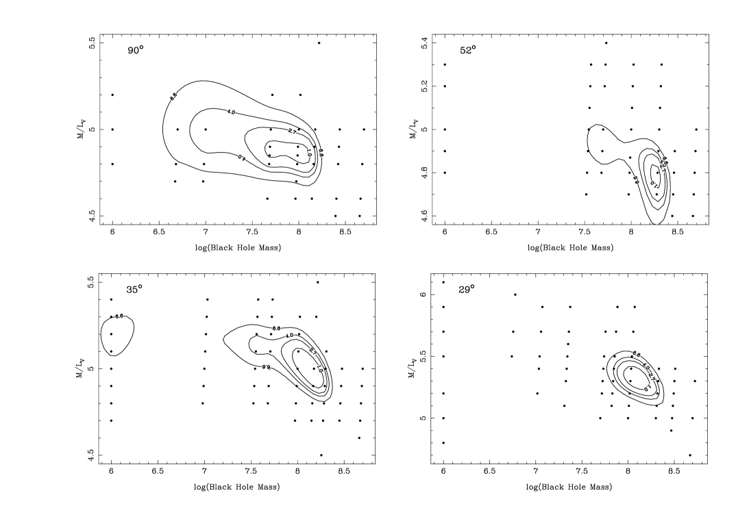
Figure 8.— Contours of $\Delta\chi^{2}$ as function of black-hole mass and M/L_V for four inclinations. The solid points represent the models that were run. The contour values are equal to $\Delta\chi^{2}=1,2.7,4.0,{\rm and}~{}6.6$; one-dimensional projection of these contours provide the 68%, 90%, 95% and 99% confidence bands respectively for the two variables, black-hole mass and M/L_V.

The total $\chi^{2}$’s for most of the models have a value near 200, giving a reduced $\chi^{2}$ of 0.3, assuming one observable equals one degree of freedom. A reduced $\chi^{2}$ near unity would require either that every three LOSVD bins are correlated by the smoothing, therefore reducing the number of degrees of freedom by three, or that the uncertainties of the bin heights are overestimated by a factor of $\sqrt{3}$. In the former case, using $\Delta\chi^{2}$ as a discriminator for the error of the best-fitting models will not be affected since the number of degrees of freedom has no influence on the calculation of the $\chi^{2}$ differences; $\Delta\chi^{2}=1$ will still correspond to 1-$\sigma$. However, in the latter case, both the $\chi^{2}$ and $\Delta\chi^{2}$ values would increase by a factor of three, creating a smaller confidence band on the variables; $\Delta\chi^{2}=1/3$ would then correspond to 1-$\sigma$. It is likely, however, that the dominant reason for the low reduced $\chi^{2}$ is the underestimation of the degrees of freedom since we know a priori that the smoothing must have an effect. To provide a quick check on smoothing effects, we refit the LOSVDs for a subset of positions using a much smaller smoothing length. As expected, the LOSVD becomes noisier. Measuring the $\chi^{2}$ between this new LOSVD and the model that we fit using the the older LOSVD, we find that the increase in $\chi^{2}$ ranges from 3-5. Thus, we conclude that the dominant effect of the smoothing is to correlate the variables and reduce the number of degrees of freedom. In retrospect, it would have been better not to have smoothed the LOSVDs and preserve their statistical independence. Note however that our decision to accept $\Delta\chi^{2}=1$ as the 1-$\sigma$ error is conservative and, if anything, overestimates the errors.

4.2. Model Fits

We examined models with inclinations from 29° to 90° (intrinsic E5 to E1 galaxy), black holes from zero to $10^{9}M_{\odot}$, and M/L_V from 4.0 to 8.0 in solar units. The $\chi^{2}$ is a function of these three variables. For each inclination, Fig. 7 plots $\chi^{2}$ as a function of black-hole mass (zero black-hole mass is shown as $10^{6}$), using that M/L_V which provides the smallest $\chi^{2}$ at that black-hole mass. All inclinations show a minimum $\chi^{2}$ at black-hole masses in the range $6\times 10^{7}-2\times 10^{8}M_{\odot}$. The fits clearly prefer the edge-on models (90°). Fig. 8 presents contours of $\Delta\chi^{2}$ as a function of black-hole mass and M/L_V for each inclination. The points represent locations of the modeled values. The contours use a two dimensional smoothing spline (Wahba 1980) to estimate the $\chi^{2}$ values at positions where no models occur. As in Wahba, Generalized Cross-Validation determines the smoothing value; however, the modeled values are relatively smooth and little smoothing is necessary.

$\chi^{2}$ as function of black hole mass for various inclinations. The labels give the inclination and the intrinsic galaxy shape. We have added $10^{6}M_{\odot}$ to the models with no black hole to put them on the log scale.

Since we have such a large parameter space—minimizing several thousand variables—we must ensure that the modeling program is finding a true minimum. Furthermore, we require that the numeric noise caused by the minimizer be smaller than the quoted uncertainties of the output parameters (e.g., the black hole mass). The two conditions that govern these checks are the sampling densities that we use in parameter space, and the tolerance used to determine convergence in the minimizer. Fig. 8 demonstrates the sampling densities for the black-hole mass and the M/L_V, where each point represents one model. Fig. 7 shows the range and number of modeled inclinations. The smoothness of the $\chi^{2}$ contours in both figures demonstrate that we have found the global minimum. As a further check, we have run models with both larger and smaller M/L_V than those presented, however the fits are significantly worse and we do not include them in the plots. Thus, we conclude that the sampling density provides adequate coverage around the global minimum. Our second concern is whether the tolerance used for the stopping criteria in the minimizer creates significant noise for the parameter estimation. We must use a stopping tolerance in the program or the time it takes for the $\chi^{2}$ to asymptote becomes impractically long. Both Figures 7 and 8 provide an estimate of the numeric noise. From the soothness of plots, the change in $\chi^{2}$ between two adjacent points is much smaller than the global change in $\chi^{2}$. Also, in a handful of models, we iterate till there is no change in $\chi^{2}$ relative to machine precision, and find that this asymptotic value is within $\Delta\chi^{2}=0.02$ of the stopping value. Therefore, the noise in $\chi^{2}$ generated from the minimization routine is not significant. The smoothness is the solution is also seen in Fig. 9, where we plot best-fit black hole mass as a function of inclination. Although, the sampling of points is not dense, the fact that there are no abrupt changes signifies we are not subject to numeric noise in the solution.

The best-fit black-hole mass as a function of inclination.

Internal dynamics of NGC 3379 for the preferred model, $1\times 10^{8}~{}M_{\odot}$ black hole, inclination 90°. The top plot shows the three internal dispersions along the major axis; the bottom plot shows the mean velocity in the equatorial plane.

As described in §3.1, we have also run models with M/L_V increasing 25% log-linearly with radius towards the galaxy center. In this case, the required M/L_V is systematically lower than when using the constant M/L_V assumption; however, the results for the required black hole and inclination are unchanged.

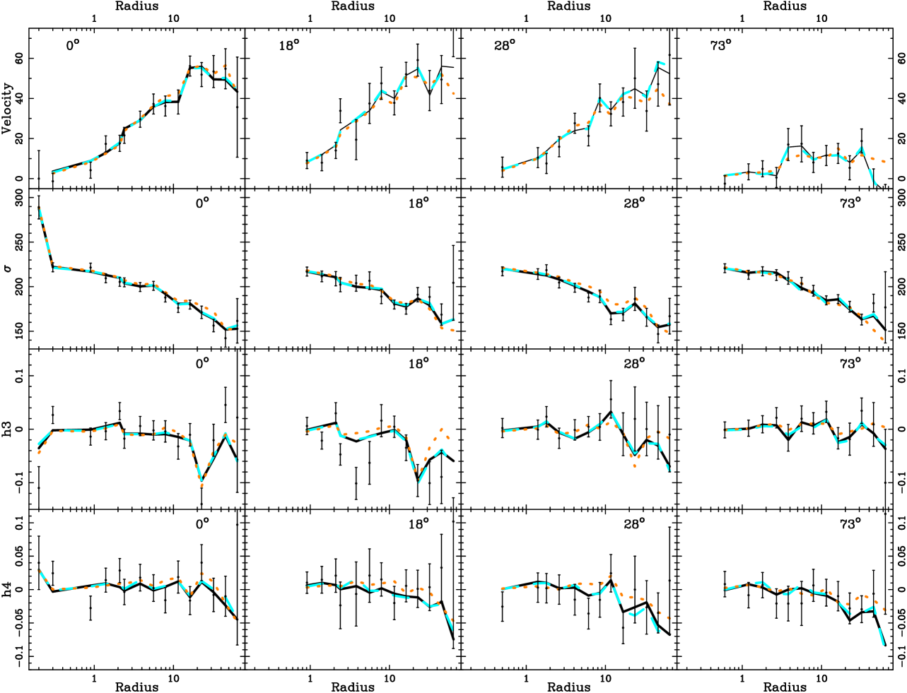
Figure 9.— Gauss-Hermite moments for data—the points with 68% error bars—and models. The solid line is the best-fit edge-on black-hole model, the dased blue line is the edge-on no-black-hole model, and the dotted orange line is the best-fit 29° model. Each column represents a different position angle which is measured up from the major axis.

The best model has an inclination of 90°, a black hole mass of $1\times 10^{8}M_{\odot}$, and M/L_V$=4.85$. The allowed mass of black holes range from $6\times 10^{7}-2\times 10^{8}M_{\odot}$. The internal dynamics of the best-fitting model are shown in Fig. 10. The top plot shows the internal velocity dispersions of the three components along the major axis. The model is tangentially biased (in the $\phi$ direction) in the smallest bin, radially biased in the mid-range radii, and tangentially biased again at the largest radii. Independent of inclination, Fig. 10 well characterizes the orbital distribution for each of the best-fitting models. Similarly, the mean velocity in the equatorial plane (bottom plot of Fig. 10) has a general shape for the best models; it shows no systematic trends from $0.4-30\arcsec$ (20-1500 pc), increasing significantly in the center due to the presence of the massive black hole. Beyond about 60″ the model is unconstrained since there is no kinematic information, but we plot the model results there since they represent the maximum entropy configuration. For each inclination the trend with black-hole mass is as follows: increasing the black-hole mass requires an increased amount of tangential anisotropy in the central bin, a decrease of the radial bias in the mid-range radii, and the orbits at the largest radii to become more isotropic. The coupling between the black-hole mass and the amount of radial anisotropy in the mid-radii stems from the need to match the same central LOSVD; a large central dispersion can be modeled with a large black-hole mass or radial orbits. Therefore, as the black-hole mass increases, the need for radial orbits decreases. In the very central bin, a large black-hole mass induces large rotational velocities and also large dispersion in the $\phi$ direction. At the largest radii, the situation is more complex since we have not included a dark halo; if the projected dispersion is larger than the dispersion obtained assuming isotropy and the stellar mass profile then one can either invoke a dark halo or include tangential anisotropy. In any event, it is not clear whether meaningful analysis at large radii can be obtained from models which do not include a dark halo.

To demonstrate why the data seem to prefer an edge-on model that contains a black hole, we must look at the model fits to the data. Figure 11 plots Gauss-Hermite polynomial estimates for the data and model LOSVDs for all four position angles. The difference between the edge-on model and the nearly face-on model is almost entirely at large radii; the edge-on model matches the large-radial data better, specifically for the velocity and velocity dispersion. In contrast, the difference between the no-black-hole and black-hole model is so subtle that one can barely discriminate those two models in Fig. 11. Only in the central bin does the the black-hole model slightly better estimate the skewness in the profile. However, Fig. 11 is not the optimal way to compare models since the fit uses the full LOSVD and not moments. Instead of plotting all 54 LOSVDs for various models, Fig. 12 plots the difference in $\chi^{2}$ at each spatial position. This difference represents the $\chi^{2}$ measured for the LOSVD of a particular model minus that of the best-fit model (edge-on, black-hole model). The two comparison models are the same as in Fig. 11, the best no-black-hole model (an edge-on model) and a nearly face-on black-hole model (at 29°). As expected, the discrimination between black-hole/no-black-hole comes mainly from the HST/FOS data point. A no-black-hole model fails to match the shape of the central LOSVD; however, there is a limit to size of the central black hole since very high black-hole masses models over shoot the dispersions in the central few ground-based measurements. Without the HST data point, we would not have been able to determine whether a black hole exists in NGC 3379. The discrimination for the inclination comes from the data at larger radii; here, the edge-on model is much better able to match the projected kinematics. As we discuss later, this inclination constraint is uncertain due to our assumption of constant M/L_V.

The change in $\chi^{2}$ relative to the best-fitted model. Each panel represents a different observed position angle. The solid line represents the $\chi^{2}$ difference for the edge-on no-black-hole model, and the dashed line represents the 29° model with a $10^{8}M_{\odot}$ black hole.

There is an uncertainty in the absolute wavelength calibration of the HST spectrum. Since we do not assume that the central HST LOSVD is symmetric, we must determine the velocity zeropoint of this profile relative to the rest frame of the galaxy ($920\pm 10$ $\rm{km}~{}\rm s^{-1}$, Borne et al. 1994). Unfortunately, our original observing strategy did not include an accurate wavelength calibration, since we were concerned mainly with the central dispersion, and thus did not obtain the necessary flanking arc-lamp spectra. We therefore tried a range of velocity zeropoints, models with velocity offsets from $0-50$ $\rm{km}~{}\rm s^{-1}$. As the offset increases, the lower limit on the black-hole mass grows, whereas the upper limit remains the same. We are not able to fit acceptable models with offsets greater than 15 $\rm{km}~{}\rm s^{-1}$. Therefore, our allowed range of black hole masses is largest using the 0 $\rm{km}~{}\rm s^{-1}$ velocity offset. All of the figures contain the results using this value.

5. Discussion

The models in this paper depend primarily on the input black-hole mass, inclination, and M/L assumption. A difficulty is that different combinations of these variables can have similar appearances in the projected kinematics. For example, the inclination and the M/L variation both affect the fit at large radii; one can easily see how differently inclined models of the same flattened galaxy will have markedly different projected dispersion profiles, and also the dispersion profile is obviously influenced by the inclusion and shape of a dark halo. Thus, by varying the shape and amount of dark halo one may be able to mimic the effect of changing the inclination. Since we have not explored a full range of halo models, we will not make strong claims as to our ability to constrain the inclination of the galaxy. However, the black hole mass is mainly driven by the data at small radii, and primarily by the HST/FOS data point. Fig. 9 demonstrates this independence from the inclination, as our best-fit black hole mass does not depend strongly on the inclination. An even more robust measurement is the orbital structure. As either the inclination or the black-hole mass varies, we find a similar velocity ellipsoid; at the smallest bin the velocity ellipsoid is mainly tangential, becoming radial in mid-range radii, and tangential again at the largest radii. Fig. 13 plots the radial motion relative to the tangential motion for four models at different inclinations. Determination of the inclination, black-hole mass, and orbital structure is discussed in detail below.

Radial relative to tangential dispersion as a function of radius along the major axis for the best-fit models at the specified inclination. The tangential dispersion is defined as $\sigma_{\rm tangential}^{2}=(\sigma_{\theta}^{2}+\sigma_{\phi}^{2})/2$.

The inclination of NGC 3379 has been the subject of some debate. Capaccioli et al. (1991) conclude that NGC 3379 is similar to NGC 3115 but nearly face-on, with some degree of triaxiality. Capaccioli base this conclusion only on the surface brightness profile and use no kinematic data. In contrast, Statler (1994) concludes that nearly face-on, triaxial models are inconsistent with the data at the 98% confidence limit, strongly contradicting Capaccioli’s result. He prefers less-inclined models. Statler has obtained more recent data (Statler & Smecker-Hane, 1999) and a fuller analysis is in preparation.

As seen in Sect. 4, our best models prefer an edge-on configuration. Preference for edge-on models arises from two observations; first, the dispersion profiles along different axes are slightly different, and, in an axisymmetric case, this configuration is not possible for a face-on system. The difference mainly arises from the inability to match the large radial data, however the face-on model also cannot match the shoulder in the dispersion profile at 10–20″ (previously noted by Statler & Smecker-Hane, 1999); the shoulder is more pronounced in the central position angles, and the edge-one models match this configuration well (see Fig. 11). Second, major-axis rotation exists which is not allowed for a face-on configuration of an oblate axisymmetric system. Thus these two restrictions are mainly a result of our axisymmetry assumption.

More general models can be constructed than those presented here. We could in principle extend the modeling technique to include triaxial distributions but then the parameter space becomes too large for us to search (each axisymmetric model takes approximately 20 hours on an Ultrasparc). Second, our assumption that the galaxy is spheroidal could be relaxed. Romanowsky & Kochanek (1997) present a technique which provides a range of different density distributions which similarly project. Third, we have assumed that M/L_V is independent of radius (i.e., there is no dark halo). Ciardullo et al. (1993), using radial velocity measurements of planetary nebulae, find no evidence for a dark halo in NGC 3379 out to 3.5 effective radii (120″); however their uncertainties are large and could, in fact, allow for some dark halo (Tremblay et al. 1995). In all of our models, the last velocity dispersion measurement (at 64″) along each position angle is higher than the model velocity dispersion, possibly suggesting the need for an increase in M/L_V. At one effective radius (34″), there is no need for an increase in M/L_V, which is consistent with previous studies of other galaxies (Kormendy & Westphal 1989, Kormendy & Richstone 1992, Kormendy et al. 1997). Thus, assumptions of axisymmetry, spheroidal distribution, and constant M/L_V all lead to uncertainties in the best-fit inclination. Detailed modeling including dark halos has been carried out by Rix et al. (1998) for NGC 2434 and Saglia et al. (1999) for NGC 1399, but only as spherical systems. Only by allowing for axisymmetric or triaxial shapes with a dark halo can we set more realistic limits on inclination.

Even though we are not able to place limits on the inclination, we can measure black-hole limits. The presence of a dark halo will have no effect on the need for a central black hole, or on its mass. The need for the black hole is directly a result of the shape of the central LOSVD observed with HST. The large dispersion and the skewness drive the models to require a black hole. We have also run models assuming a symmetrized central LOSVD (the dashed line shown in Fig. 4). The allowable range of black hole masses remains the same for the inclined models in this case. However, for the edge-on case the model with no black hole fits as well. The symmetrized LOSVD has a dispersion of 275 $\rm{km}~{}\rm s^{-1}$, compared with 289 $\rm{km}~{}\rm s^{-1}$ for the actual LOSVD, and has less tail weight (as can be seen in Fig. 4). These differences permit a no-black-hole model. The central bin most influences the model; most of the orbits ($>70$% for inclined models and $>95$% for edge-on models) contribute light to this bin, and, furthermore, many have their pericenter there. Therefore, the characteristics of the central LOSVD, in particular the high-velocity components, have a strong effect on orbits throughout the galaxy. In the edge-on case with the symmetrized LOSVD, the orbits redistribute themselves in such a way as to create a slightly larger central dispersion (275 $\rm{km}~{}\rm s^{-1}$) without the need for a black hole, and at the same time maintain a fairly flat projected dispersion profile; i.e., at small radii, the orbits are mainly radial, whereas at large radii they become primarily tangential. However, the actual LOSVD warrants matching the skewness and the high-velocity tails. With no black hole present, the model must use stars at larger radii to create the high-velocity components, thereby limiting its ability to redistribute the orbits at large radii and match the kinematics there. With a black hole, the black hole provides much of the high-velocity tail of the LOSVD for orbits locally and gives the model more freedom to better match the larger-radii data. The symmetrized and skewed LOSVDs are inconsistent with each other with greater than 95% probability, both using an estimate from the binned values and using the Gauss-Hermite moments. Given the arguments in §2.2.1, we must include the skewness of the central LOSVD and thus do not consider the symmetrized LOSVD models further.

Relaxing the other two assumptions—axisymmetry and spheroidal distribution–is unlikely to change the black-hole limits. The models with no black holes all are extremely poor fits to the data; therefore, even if we allow for the variation in deprojected densities given by Romanowsky & Kochanek, the results are unlikely to change. Of course, since the deprojection is unique for the edge-on models, our results are general in the edge-on case. Triaxial models will allow even greater freedom to match the data, however it is not clear whether triaxiality is a viable configuration in the centers of galaxies (Merritt& Fridman 1996, Merritt 1999), and we do not consider these models.

The position angle of the dust ring in Fig. 5 is 45° away from the major axis of the galaxy. A dust ring in an axisymmetric system with an offset position angle is only neutrally stable but can be stabilized by a small amount of triaxiality. If the galaxy is nearly face-on, then triaxiality is not necessary to stabilize the dust ring; in the face-on configuration, since the dust ring is close to edge-on (about 75°), it must be in an orbit close to polar, and thus can have arbitrary azimuthal angle. Velocity information along the dust ring could provide an important check on the enclosed mass derived from our models.

Pastoriza et al. (1999), using ground-based gas kinematics, assume that the gas disk in NGC 3379 is nearly face-on. Their mass estimate inside 1.3″ is $7\times 10^{9}M_{\odot}$, strongly contradicting our result. However, their large mass is due mainly to their disk inclination assumption. If one uses the inclination as measured from the dust ring, then the enclosed mass closely equals our value of $1\times 10^{8}M_{\odot}$; only with HST can we precisely determine the gaseous disk configuration and determine whether the gas is even in a disk at all. The HST/FOS spectrum includes the [NII] emissiom, although since it is a single pointing, we do not have the radial information to extract a meaningful dynamical analysis from the gas. However, the width of the line does provide some information on the underlying mass. The measured $\sigma$ is 200$\rm{km}~{}\rm s^{-1}$, in agreement with the mass deduced here; using the mass from Pastoriza et al. would imply a $\sigma$ around 700$\rm{km}~{}\rm s^{-1}$. To further understand the gas kinematics, we must have spatial information.

Van der Marel et al. (1990) apply 2-integral flattened models for NGC 3379 using constant anisotropy. They find an acceptable fit with an inclination of 60° and anisotropic orbits. They suffer from the same problem as we do for the inclination estimate; without inclusion of a dark halo it is not possible to obtain adequate inclination constraints. Furthermore, since our axisymmetric models are fully general while their models specify a form for the distribution function, we cannot directly compare our results to theirs. Van der Marel et al. conclude that there is no evidence to support the need for a third integral using data from the first and second moments of the LOSVD from Davies & Birkinshaw (1988). Results presented here, which are based on higher S/N data and are determined from the full LOSVD, show that the best model requires three integrals and is not consistent with a 2-integral distribution function; the internal dispersions along the long axis in the radial and $\theta$ directions are significantly different, in direct conflict with a 2-integral distribution function. As seen in Fig. 13, the ratio of the $\theta$ to the radial dispersion in our best model have a radial variation from 0.6 to 1.2, with an average around 0.75. For comparison, this ratio is around 0.6 for the spheroid component of our Galaxy using RR Lyrae halo stars (Layden 1995).

In addition to the measured black-hole mass, the orbital structure appears to be a robust feature as well. The radial anisotropy profile along the major axis in Fig. 13 shows that this profile is nearly independent of input inclination. For all acceptable models, the velocity ellipsoid is tangentially biased in the central bin and radially biased in the mid-range radii. These orbital properties are generally true along any position angle. This central tangential bias appears in other 3-integral models studied (Gebhardt et al. 2000) and may be a common feature of early-type galaxies. Tangential bias in the central regions around black holes appear to be a common feature in simulations (Quinlan et al. 1995, Quinlan & Hernquist 1997, Merritt & Quinlan (1998), and Nakano & Makino 1999). The radial bias in the mid-range radii has also been seen before; using 3-integral models, both Gerhard et al. (1999) for NGC 1600 and Saglia et al. (1999) for NGC 1399 find radial motion throughout the main body of the galaxy. Thus, we may be beginning to measure common features of the orbital properties in ellipticals—tangential motion in the central regions and radial motion at mid-range radii. At large radii, we must include dark halos since they make a significant contribution there. The next step is to determine dominant evolutionary effects from theoretical models and will require detailed comparisons with N-body simulations.

Magorrian et al. (1998), using the same ground-based data, fit two-integral models to the observed second-order velocity moment profiles and require a BH of $3.9^{+0.3}_{-0.4}\times 10^{8}M_{\odot}$. Our more general three-integral models would allow an even larger range of BH masses had we similarly used only the LOSVD’s second moments. When we fit to the full LOSVDs, however, their shape requires that our models be mildly radially anisotropic, reducing the required BH mass by a factor of at least two over Magorrian et al.’s result. The models presented in this paper still contain restrictive assumptions—namely constant M/L_V and spheroidal symmetry—requiring yet more models to study black hole properties in complete generality.

Kormendy (1993) and Kormendy & Richstone (1995) find that there is a correlation between the black hole mass and the mass of the spheroid. Whether this relation is a real correlation or an upper envelope that extends to smaller black-hole masses remains to be seen. As the data quality and the modeling techniques improve, we should be better able to constrain the relationship between black hole and spheroid mass, and begin to measure correlations with the orbital characteristics.

Table 1NGC 3379 HST Photometry Results

$R$ (″)	$V$	$V-I$	$e$	PA
0.023	14.625	1.302	0.121	92.3
0.046	14.739	1.314	0.121	92.3
0.091	14.931	1.340	0.040	92.3
0.136	14.978	1.311	0.232	92.3
0.182	15.047	1.322	0.181	101.8
0.227	15.101	1.307	0.181	87.6
0.273	15.147	1.311	0.177	87.6
0.318	15.184	1.313	0.149	85.8
0.364	15.227	1.311	0.141	84.4
0.409	15.276	1.325	0.119	84.1
0.455	15.288	1.311	0.119	78.8
0.500	15.326	1.318	0.119	76.4
0.546	15.351	1.313	0.110	64.9
0.566	15.368	1.326	0.083	58.1
0.665	15.412	1.297	0.119	65.7
0.783	15.485	1.300	0.095	58.7
0.921	15.578	1.299	0.089	69.6
1.084	15.692	1.300	0.085	67.5
1.275	15.812	1.305	0.081	70.8
1.500	15.933	1.299	0.101	70.9
1.764	16.072	1.297	0.104	72.1
2.076	16.213	1.293	0.115	73.3
2.442	16.365	1.295	0.117	74.0
2.873	16.528	1.291	0.119	73.5
3.380	16.702	1.286	0.118	73.8
3.977	16.895	1.284	0.111	74.0
4.678	17.110	1.278	0.105	74.1
5.504	17.352	1.275	0.094	74.0
6.475	17.596	1.272	0.088	73.8
7.618	17.830	1.267	0.089	73.2
8.962	18.064	1.262	0.089	73.2
10.544	18.313	1.257	0.090	72.1
12.405	18.572	1.246	0.092	71.1
14.594	18.855	1.237	0.089	69.3

References

- (1)
- (2) Ajhar, E., Lauer, T., Tonry, J., Blakeslee, J., Dressler, A., Holtzman, J., & Postman, M. 1997, AJ, 114, 626
- (3) Bender, R., 1990, A&A, 229, 441
- (4) Bender, R., Saglia, R.P., & Gerhard, O.E. 1994, MNRAS, 269, 785
- (5) Borne, K.D., Balcells, M., Hoessel, J.G, & McMaster, M. 1994, ApJ, 435, 79
- (6) Bower, G. et al. 1998, ApJ, 492, 111
- (7) Capaccioli, M., Held, E.V., & Nieto, J.L. 1987, AJ, 94, 1519
- (8) Capaccioli, M., Held, E.V., Lorenz, H. & Vietri, M. 1990, AJ, 99, 1813
- (9) Capaccioli, M., Vietri, M., Held, E.V., & Lorenz, H. 1991, ApJ, 371, 535
- (10) Carollo, C.M., de Zeeuw, P.T., van der Marel, R.P., Danziger, I.J., & Qian, E.E. 1995, ApJ, 441, L25
- (11) Ciardullo, R., Jacoby, G.H., & Dejonghe, H.B. 1993, ApJ, 414, 454
- (12) Cretton, N., de Zeeuw, P.T., van der Marel, R.P., & Rix, H.-W., 1999, ApJS, accepted
- (13) Davies, R.L., & Birkinshaw, M. 1988, ApJS, 68, 409
- (14) Dejonghe, H.B. 1987, MNRAS, 224, 13
- (15) de Vaucouleurs, G., & Capaccioli, M. 1979, ApJS, 40, 699
- (16) Faber, S.M. et al. 1997, AJ, 114, 1771
- (17) Ferrarese, L., Ford, H.C., & Jaffe, W. 1996, ApJ, 470, 444
- (18) Franx, M., Illingworth, G.D., & Heckman, T.M. 1989, ApJ, 344, 613
- (19) Gebhardt, K., Richstone, D. et al. 1996, AJ, 112, 105
- (20) Gebhardt, K., Richstone, D. 1999, in preparation
- (21) Gerhard, O.E. 1993, MNRAS, 265, 213
- (22) Gonzalez, J. 1994, PhD thesis, UCSC
- (23) Harms, R.J. et al. 1994, ApJ, 435, L35
- (24) Keyes, C. D., et al. 1995, FOS Instrument Handbook (Baltimore: STScI)
- (25) Kormendy, J. 1977, ApJ, 218, 333
- (26) Kormendy, J. 1992, in “Testing the AGN Paradigm”, eds. S.S. Holt, S.G. Neff, & C.M Urry (NY: AIP), 23
- (27) Kormendy, J. 1985, ApJ, 292, L9
- (28) Kormendy, J. 1993, in “The Nearest Active Galaxies”, eds. J. Beckman, L. Colina, & H. Netzer (Madrid), 197
- (29) Kormendy, J., & Westphal, J. 1989, ApJ, 338, 752
- (30) Kormendy, J., & Richstone, D. 1992, ApJ, 393, 559
- (31) Kormendy, J., & Richstone, D. 1995, ARA&A, 33, 581
- (32) Kormendy, J. et al. 1996,ApJ, 459, L57
- (33) Kormendy, J. et al. 1997, ApJ, 482, L139
- (34) Kormendy, J., Bender, R., Evans, A., & Richstone, D. 1998, AJ, 115, 1823
- (35) Lauer, T.R. 1985, MNRAS, 216, 429
- (36) Lauer, T.R. et al. 1995, AJ, 110, 2622
- (37) Layden, A.C. 1995, AJ, 110, 2288
- (38) Magorrian, J. et al. 1998, AJ, 115, 2285
- (39) Merritt, D. 1997, AJ, 114, 228
- (40) Merritt, D. 1999, PASP, 111, 129
- (41) Merritt, D., & Fridman, T. 1996, ApJ, 460, 136
- (42) Nakano, T., & Makino, J. 1999, ApJ, 510, 155
- (43) Pastoriza, M., Winge, C., Ferrari, F., & Macchetto, D. 1999, ApJ, accepted
- (44) Peletier, R.F., Davies, R.L., Illingworth, G.D., Davis, L.E., Cawson, M. 1990, AJ, 100, 1091
- (45) Qian, E.E., de Zeeuw, P.T., van der Marel, R.P., & Hunter, C. 1995, MNRAS, 274, 602
- (46) Quinlan, G., Hernquist, L., & Sigurdsson, S. 1995, ApJ, 440, 554
- (47) Quinlan, G., & Hernquist, L. 1997, NewA, 2, 533
- (48) Richstone, D., Gebhardt, K. et al. 1999, in preparation
- (49) Richstone, D., & Tremaine, S. 1988, ApJ, 327, 82
- (50) Rix, H.-W., de Zeeuw, P.T., Carollo, C.M., Cretton, N., & van der Marel, R.P. 1997, ApJ, in press
- (51) Romanowsky, A., Kochanek, C. 1997, MNRAS, 287, 35
- (52) Rybicki, G.B. 1987, in Structure and Dynamics of Elliptical Galaxies, IAU Symposium 127, ed. de Zeeuw, P.T., (Reidel, Dordrecht), p.397
- (53) Ryden, B. 1996, ApJ, 461, 146
- (54) Saha, P., & Williams, T.B. 1994, AJ, 107, 129
- (55) Schwarzschild, M. 1979, ApJ, 232, 236
- (56) Statler, T.S. 1994, AJ, 108, 111
- (57) Statler, T.S., & Smecker-Hane, T. 1999, AJ, Feb. 1999
- (58) Tremblay, B., & Merritt, D., & Williams, T.B. 1995, ApJ, 443, L5
- (59) van der Marel, R.P., Binney, J.J., & Davies, R.L. 1990, MNRAS, 245, 582
- (60) van der Marel, R.P. 1991, MNRAS, 253, 710
- (61) van der Marel, R.P., & Franx, M. 1993, ApJ, 407, 525
- (62) van der Marel, R.P., Cretton, N., de Zeeuw, P.T., & Rix, H.-W. 1998, ApJ, 493, 613
- (63) van Dokkum, P.G., & Franx, M. 1995, AJ, 110, 2027
- (64) Wahba, G. 1980, Technical Report No. 595, Univ. of Wisconsin
- (65) Worthey, G. 1994, ApJS, 95, 107
- (66)