FEEDBACK FROM GALAXY FORMATION: ESCAPING IONIZING RADIATION FROM GALAXIES AT HIGH REDSHIFT

Abstract

Several observational and theoretical arguments suggest that starburst galaxies may rival quasars as sources of metagalactic ionizing radiation at redshifts $z>3$. Reionization of the intergalactic medium (IGM) at $z>5$ may arise, in part, from the first luminous massive stars. To be an important source of radiative feedback from star formation, a substantial fraction ($\sim 1-10$%) of the ionizing photons must escape the gas layers of the galaxies. Using models of smoothly distributed gas confined by dark-matter (DM) potentials, we estimate the fraction, $\langle f_{esc}\rangle$, of Lyc flux that escapes the halos of spherical galaxies as a function of their mass and virialization redshift. The gas density profile is found by solving the equation of hydrostatic equilibrium for the baryonic matter in the potential well of a DM halo with the density profile found by Navarro et al. (1996). We then perform a parametric study to understand the dependence of $\langle f_{esc}\rangle$ on redshift, mass, baryonic fraction, star-formation efficiency (SFE), stellar density distribution, and OB association luminosity function. We give useful analytical formulas for $\langle f_{esc}(z,M_{DM})\rangle$. Using the Press-Schechter formalism, we find that stellar reionization at $z\sim 7$ is probably dominated by small galactic sub-units, with $M_{DM}\lower 2.15277pt\hbox{$\;\buildrel<\over{\sim}\;$}10^{7}$ M_⊙ and SFE $\sim 10$ times that in the Milky Way. This may affect the distribution of heavy elements throughout the intergalactic medium.

1 Introduction

In all cosmological models, the temperature of the cosmic background radiation at redshift $z\sim 1000$ is sufficiently low that hydrogen ions recombine and radiation decouples from matter. The baryonic Jeans mass after this event is $\sim 10^{5}$ M_⊙, and the first luminous objects in a CDM cosmology could form at redshift $z\simeq 30$ (Peebles & Dicke, 1968; Binney, 1977; Rees & Ostriker, 1977; Silk, 1977; White & Rees, 1978; Tegmark et al., 1996; Abel et al., 1998). If fragmentation occurs, triggered by H₂ formation and radiative cooling (Lepp & Shull, 1984; Abel et al., 1998), massive stars are likely to form. Depending on the slope of the initial mass function (IMF) and on the star-formation efficiency (SFE), the massive-star population will be a source of mechanical energy, heavy elements, and Lyman continuum (Lyc) photons. Such processes are known as “feedback” from galaxy formation, and they can have substantial impact on the intergalactic medium (IGM) and on future generations of stars and galaxies.

In this paper, we focus on radiative feedback in the form of ionizing radiation from massive stars. In addition to its effects on diffuse gas in the halos of galaxies, Lyc radiation from the first stars can also provide an important source for ionizing the surrounding IGM (Madau & Shull, 1996). Observations of the transmitted flux below the Ly$\alpha$ emission line in high-redshift quasars (the Gunn-Peterson effect) imply that the diffuse IGM was already ionized at redshift $z=5$. Although QSOs play a dominant role in photoionizing the IGM at $z<4$ (Shapiro & Giroux, 1987; Donahue & Shull, 1987; Meiksin & Madau, 1993), their dwindling numbers at $z>4$ (Pei, 1995; Miralda-Escudé & Ostriker, 1990; Madau, 1998; Fardal et al., 1998) suggest the need for another ionization source. Unless a hidden population of quasars is found, radiation emitted by high-redshift massive stars seems necessary to reionize the universe. This hypothesis is reinforced by recent observations of He II absorption (Reimers et al., 1997), from the redshift evolution of the column density ratio of Si IV/C IV and C II/C IV in the Ly$\alpha$ forest (Songaila & Cowie, 1996; Boksenberg, 1997), and form the thermal history of the IGM (Ricotti et al., 2000; Schaye et al., 1999) that favor a soft spectrum of the ionizing radiation, more typical of hot stars than of quasars (Haardt & Madau, 1996; Fardal et al., 1998).

A key ingredient in determining the effectiveness by which starburst galaxies photoionize the surrounding IGM is the parameter $\langle f_{esc}\rangle$, the escaping fraction of Lyc photons. This factor depends on the shape of the galaxy, on the gas and stellar density profiles, and on the IMF and SFE. Recent estimates (Madau & Shull, 1996) suggest that if 10% of the ionizing photons from hot stars escape the disk gas layers [$\langle f_{esc}\rangle$ $\approx 0.1$], starbursts can rival QSOs as sources of the metagalactic background at $z>3$. Haiman & Loeb (1997) made a coarse estimate of $\langle f_{esc}\rangle$ for spherical objects of different masses at various redshift. They provided a fitting formula, $\log\langle f_{esc}\rangle=1.92\exp[-(z-10)^{2}/1510]-1$, valid for $z>10$, and chose a value $\langle f_{esc}\rangle$ $\simeq 1$ for $z<10$. However, these estimates are not based on any secure calculation or observation and we do not reproduce their results.

Theoretical models (Dove & Shull, 1994, hereafter DS94) of the radiative transfer of Lyc radiation through disk layers of a spiral galaxy like the Milky Way suggest that $\langle f_{esc}\rangle$ could range from 5–20%. The DS94 calculation considered only “burn-through”: photoionized channels (H II regions) produced in smoothly distributed gas layers in hydrostatic equilibrium. More realistic models must include gas dynamics and radiative transfer through a network of radiatively ionized H II regions and superbubble-driven cavities (“chimneys”) of hot gas (Norman & Ikeuchi, 1989). By solving the time-dependent radiation transfer of stellar radiation through evolving superbubbles, Dove et al. (2000) found that superbubbles reduce the escape fraction to $\langle f_{esc}\rangle$ $\sim 6\%$ because the shells of the expanding superbubbles can trap or attenuate the ionizing flux. By the time that the superbubbles of large associations blow out of the H I disk, the ionizing photon luminosity has dropped well below the maximum luminosity of the OB association. Observational limits on the transmitted flux from four low-redshift galaxies studied by the Hopkins Ultraviolet Telescope (HUT) are consistent with $\langle f_{esc}\rangle$ ranging from a few percent up to $50\%$. By comparing the observed number of Lyc photons with a set of theoretical spectral energy distributions for the galaxies, Leitherer et al. (1995) derived, on average, $\langle f_{esc}\rangle$ $\leq 3\%$. Reexamining the same observations, Hurwitz et al. (1997) derived larger upper limits on the escape fraction ($5.2\%$, $11\%$, $57\%$, and $3.2\%$) for the four galaxies. Absorption from undetected interstellar components could allow the true escape fractions to exceed these upper limits.

In this paper, we attempt to provide a more realistic estimate of the production rate and escape fraction of Lyc from high-$z$ galaxies. We estimate the fraction of Lyc flux escaping the halo of spherical galaxies as a function of their mass, integrated ionizing flux emitted by the hot star population, and virialization redshift of their dark-matter halos. In § 2 we describe the method used to estimate the escape fraction, and in § 3 we show the results of the simulations. In § 4 we use a Press-Schechter estimate of the distribution of virialized dark-matter halos to estimate the emissivity from galaxies as a function of redshift. Reionization from the first stars appears to be dominated by small objects with $M_{DM}\leq 10^{7}~{}M_{\odot}$. Finally, in § 5 we summarize and discuss our results.

2 Method

We study the Lyc escape fraction from a spherical galaxy as a function of its virialization redshift, dark matter mass, baryonic fraction and total Lyc photon flux, $S_{tot}$. We also consider the case of $S_{tot}$ proportional to the baryonic content of the galaxy, and we derive from simulations analytical expressions of $\langle f_{esc}\rangle$ for both cases.

We use a Monte-Carlo method to simulate the radial distribution of OB associations in a spherical galaxy. In our fiducial model (see § 2.2), we adopt a constant stellar probability distribution as a function of radius, with a sharp stellar cutoff at the core radius of the dark matter halo. In § 3.3 we relax this assumption, exploring the cases of a stellar density distribution that follows the baryonic mass distribution and the Schmidt Law. We also estimate $\langle f_{esc}\rangle$ for the cases when the stars are located at the center of the halo and when the sharp stellar cutoff is set to a critical baryonic density, $n_{b}=1$ and 10 cm^-3. We then calculate $f_{esc}(S)$ for each OB association as a function of its Lyc photon luminosity, $S$ (photons s^-1), and its location in the galaxy. We calculate the number of OB associations with luminosities $S-\Delta S/2<S<S+\Delta S/2$ integrating the luminosity function from the lower to the upper cutoff of the luminosity function, normalized to the total Lyc photon luminosity. Since we do not use a Monte-Carlo method but a simple integration, the actual upper cutoff of the luminosity distribution depends on the total Lyc flux. In the fiducial model the luminosity function is $dN_{a}(S_{0})/dS_{0}\propto S_{0}^{-2}$ for $10^{48}\leq S_{0}\leq 10^{51}$ s^-1, but in § 3.4 we study the dependence of $\langle f_{esc}\rangle$ on the assumed luminosity function of the OB associations. Finally, we sum all contributions to find $\langle f_{esc}\rangle$ for the whole galaxy, taking care of averaging the results for several Monte-Carlo realizations of the same simulation.

The method used to derive the escaping flux for a single OB association is analogous to that described in DS94, except that we consider a spherical galaxy instead of a disk galaxy. Thus, we have an additional degree of freedom, the distance $R$ of the OB associations from the center of the halo. We assume that a single OB association is a point source of Lyc photons and that the gas is in ionization equilibrium. Since the hot stars may lie off galactic center, the shape of the H II region is not spherical and is determined by equating the number of photoionizations with radiative recombinations along each ray. Along a given ray, the Strömgren radius, $r_{s}$, is defined by:

$${S_{0}\over 4\pi\alpha_{H}^{(2)}}=\int_{0}^{r_{s}}n_{H}^{2}(R)r^{2}dr\;,$$ (1)

where $S_{0}$ is the unattenuated Lyc photon luminosity of the OB association (s^-1), $n_{H}$ is the hydrogen number density, and $\alpha_{H}^{(2)}$ is the hydrogen case-B recombination coefficient. We assume that the gas inside the H II region is isothermal at $T=10^{4}$ K [$\alpha_{H}^{(2)}=2.59\times 10^{-13}$ cm³ s^-1]. The density profile of the baryonic matter is determined by solving the hydrostatic equilibrium of the gas in the potential well of the DM halo. We assume a spherically symmetric halo, so the density dependence is only on $R$. If the OB association lies off center at a distance $D$, in a polar coordinate system ($r,\theta$) with the OB association centered at the origin of axes and the $y$-axis intersecting the center of the halo, we have $R=(D^{2}+r^{2}+2Dr\sin\theta)^{1/2}$. In Figure 1 we draw a sketch showing the galaxy halo with the system of reference and the notations used in the text.

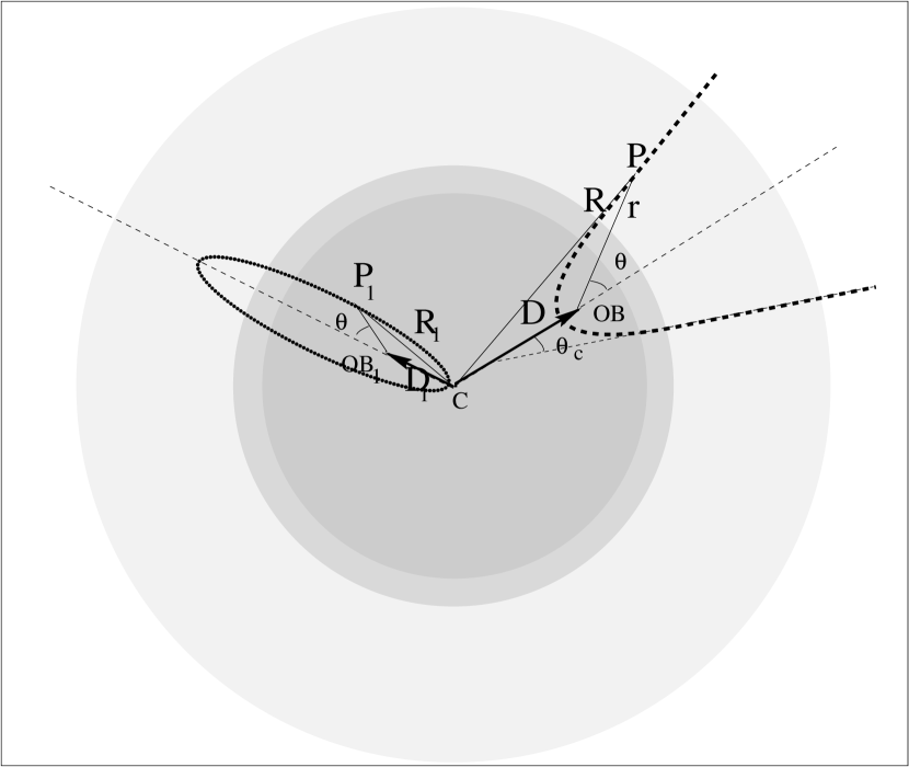
Figure 1: Sketch showing the galaxy halo with the system of reference and the notations used in the text. The OB association has a distance $D$ from the center of the halo, and the density is a function of the radius $R$. The critical angle, $\theta_{c}$, is defined for the ($r,\theta$) polar coordinate system centered on the OB association.

The fraction of Lyc photons escaping the halo is given by integrating over solid angle the fraction $f(\theta)d\theta$ of Lyc photons emitted between angles $\theta$ and $\theta+d\theta$ that are not absorbed by the H I in the halo:

$$\eta_{esc}(S_{0})={1\over 4\pi}\int_{0}^{\theta_{c}(S_{0})}f(\theta)2\pi\sin\theta\,d\theta\;,$$ (2)

where $\theta_{c}$ is the critical angle [$f(\theta_{c})=0$] for escape (Figure 1) and

$$f(\theta)=1-{4\pi\alpha_{H}^{(2)}\over S_{0}}\int_{0}^{\infty}n_{H}^{2}(R)r^{2}dr\;.$$ (3)

2.1 Barionic mass distribution

The spherical nonlinear model for gravity perturbations predicts that a just-virialized gas cloud has an overdensity (“collapse factor”) of $\Delta_{c}(\Omega_{m},\Lambda)=18\pi^{2}\approx 178$ and is shock heated to the virial temperature. Thus, the baryonic gas that virializes into the DM halo of mass $M_{DM}$ at redshift $z_{vir}$ has average hydrogen number density $\overline{n}_{vir}$, virial radius $R_{vir}$ (following convention, this is also called $R_{200}$, where one approximates 178 by 200), and temperature $T_{vir}$ given by:

$$\overline{n}_{vir} \sim 0.03~{}{\rm cm}^{-3}\left({\Omega_{b}h^{2}\over 0.019}\right)\left({1+z_{vir}\over 10}\right)^{3},$$ (4)

$$R_{vir} \sim 344~{}{\rm pc}\left({\Omega_{m}h^{2}\over 0.15}\right)^{-1/3}\left({M_{DM}\over 10^{6}~{}{\rm M}_{\odot}}\right)^{1/3}\left({1+z_{vir}\over 10}\right)^{-1},$$ (5)

$$T_{vir} \sim 556~{}{\rm K}\left({\Omega_{m}h^{2}\over 0.15}\right)^{1/3}\left({M_{DM}\over 10^{6}~{}{\rm M}_{\odot}}\right)^{2/3}\left({1+z_{vir}\over 10}\right)\left({\mu\over 0.6m_{p}}\right),$$ (6)

where $\Omega_{m}$, $\Omega_{b}$ and $h$ have the usual meanings and $\mu$ is the mean molecular weight of the gas.

We assume a hierarchical clustering scenario for the formation of virialized halos (White & Frenk, 1991). The results of numerical simulations show that DM halos are well fitted by a universal profile of mass density, $\rho(R)$, valid for a wide range of halo masses. According to the results of Navarro et al. (1996, 1997) this profile is steeper than that of an isothermal sphere, $\rho(R)\propto R^{-3}$ if $R>R_{s}$ and smoother if $R<R_{s}$. Thus, we take

$$\rho_{DM}(R)={\delta_{c}~{}\rho_{c0}\over(R/R_{s})(1+R/R_{s})^{2}}\;,$$ (7)

where $\rho_{c0}=3H_{0}^{2}/8\pi G$ is the critical density of the universe at $z=0$. Integrating $\rho_{DM}(R)$, one finds that the overdensity is given by

$$\delta_{c}=(3\times 10^{3})\Omega_{m}(1+z_{vir})^{3}\;.$$ (8)

The characteristic radius, $R_{s}(M)$, of the DM is given by

$$R_{s}(M)={R_{vir}(M_{DM})\over c(M_{DM})}={1\over c(M_{DM})}\left({3M_{DM}\over 4\pi\Delta_{c}\rho_{c0}}\right)^{1\over 3}\;,$$ (9)

where $c$ is the concentration factor, $\Omega_{m}$ is the density parameter at $z=0$, $\Delta_{c}(\Omega_{m},\Lambda)$ is the collapse factor in a spherical nonlinear model, and $z_{vir}$ is the virialization redshift of the halo. The concentration parameter $c$ is related to $\delta_{c}$ by

$$\delta_{c}=\Delta_{c}\left[{c^{3}\over\ln(1+c)-c/(1+c)}\right]\;.$$ (10)

We solve the equation of hydrostatic equilibrium of the baryonic matter numerically by assuming that the gravitational effect of the baryonic matter is negligible compared to the DM. The support of the gas in the gravitational well of the DM is dominated by bulk motions at high redshifts (Abel et al., 1998). We then define an effective temperature profile that is the sum of all contributions to the pressure (turbulent pressure, ram pressure, centrifugal force). If the gas is isothermal, the equations have a simple analytical solution,

$$\rho_{g}(R)=\rho_{g0}\exp(-27b/2)\left(1+{R\over R_{s}}\right)^{27bR_{s}\over 2R}\;,$$ (11)

where $b=(2c/9\Gamma)[\ln(1+c)-c/(1+c)]^{-1}$ and where $\Gamma=T_{vir}/T_{g}\simeq 1$ measures the efficiency of shock heating of the gas. If we assume isothermality, the resulting profile is well approximated by a $\beta$-model (Makino et al., 1998),

$$\rho_{g}(R)={\rho_{g0}\over[1+(R/R_{c})^{2}]^{3\beta/2}}\;,$$ (12)

with $\beta\simeq 0.9b$ and $R_{c}\simeq 0.22R_{s}$. In Figure 2 we show the DM density profile and the baryonic matter density profile for an isothermal gas.

Figure 2: Profile of baryonic matter (BM, solid line) expected from the universal density profile of DM halo (dotted line) for an isothermal gas at virial temperature $T$ (dashed line). The radius $R_{s}=R_{200}/c$ is related to the size of the DM core, where $R_{200}$ is the virial radius and $c$ is the concentration parameter; in this plot $c=10$. The density profile of the gas is well approximated by the isothermal $\beta$-model with a core radius $R_{c}=0.22R_{s}$ and $\beta=0.9b$ ($b\sim 1$ is a function of the concentration parameter and the gas temperature).

2.2 Stellar density distribution and luminosity function

We estimate the total number of escaping Lyc photons from the galaxy by integrating the escaping radiation of each single OB association over the luminosity function of the OB associations, where the position of each association inside the halo is determined by a Monte-Carlo simulation. We assume a power law for the luminosity function, $dN_{a}(S_{0})/dS_{0}\propto S_{0}^{-\alpha}$ for $S_{1}\leq S_{0}\leq S_{2}$, where $S_{1}$ and $S_{2}$ are lower and upper limits of the observed luminosities and $\alpha=2.0\pm 0.5$, as has been determined for OB associations in 30 local spiral and irregular galaxies (Kennicutt et al., 1989). A value $\alpha=2.12\pm 0.04$ was also found for the luminosity function of young stellar clusters in the interacting Antennae galaxies (Whitmore et al., 1999). In our fiducial models, we assume $S_{1}=10^{48}$ s^-1, $S_{2}=10^{51}$ s^-1 and $\alpha=2$; for a more exhaustive discussion of this assumption, see DS94.

The flux emitted by all the OB associations is given by:

$$S_{tot}=\int_{S_{1}}^{S_{2}}S_{0}\left({dN_{a}(S_{0})\over dS_{0}}\right)dS_{0}=N_{OB}S_{1}\ln\left({S_{2}\over S_{1}}\right)=N_{OB}(6.9\times 10^{48}~{}{\rm s}^{-1})\;,$$ (13)

where $N_{OB}$ is the number of OB associations. We divide the OB associations into 10 logarithmic bins according to their luminosity. In the case of $\alpha=2$ and 10 logarithmic bins, the upper cutoff is smaller than $S_{2}$ if $S_{tot}<10\times S_{2}$.

We assume a radial density distribution for the associations. In the fiducial models we chose a random distribution in radius for the distance of the associations from the center of the halo with a cutoff at a radius $R=R_{s}$. In this region, if the gas is isothermal, the density profile is almost flat inside the core radius $R=R_{c}$ and starts to decrease near $R_{s}$ as $R^{-3}$. The average OB association density distribution then goes as $R^{-2}$ for $R=0$ to $R=R_{s}$ and is zero for $R>R_{s}$. In § 3.4 we study the dependence of $\langle f_{esc}\rangle$ on the assumed luminosity function of the OB associations, and in § 3.3 we study the effect on $\langle f_{esc}\rangle$ of different stellar density distributions and radial cutoffs.

Figure 3: Shapes of H II regions in one Monte-Carlo simulation with $N_{OB}=100$ ($S_{tot}=6.9\times 10^{50}$ photons s^-1) in a DM halo with $M_{DM}=10^{9}$ M_⊙, $R_{s}\simeq 1.1$ kpc (outer circle), and $z_{vir}=2$. The gas core radius is $R_{c}\simeq 250$ pc (inner circle), and the gas effective temperature is $T\simeq 16,000$ K. In this simulation we find $\langle f_{esc}\rangle$ $\simeq 6.5\%$.

3 Results

The cosmological model we adopt is $\Lambda$CDM with $\Omega_{m}=0.3$, $\Omega_{\Lambda}=0.7$, $h=0.7$ and $\Omega_{b}h^{2}=0.019$ (Burles & Tytler 1998). Unless otherwise stated, the DM halos are characterized by a concentration parameter $c=10$ and a collapse factor $\Delta_{c}(\Omega_{m},\Lambda)\approx 200$. We do not consider a multi-phase interstellar medium, and we neglect the effect of stellar winds and supernova explosions on the dynamics of the ISM (Dove et al., 2000). Later in this section, we discuss these approximations.

3.1 Case I: constant Lyc flux

First, we consider a constant number of OB associations (i.e., fixed $S_{tot}$), in galaxies of different masses. An example of a Monte-Carlo simulation is shown in Figure 3, and our results are shown in Figure 4. In Figure 4 (left) we show the escaping fraction as a function of the mass of the DM halo for a constant starburst that produces a total number of Lyc photons $S_{tot}=3.5\times 10^{51}$ s^-1. Each point is the mean of five Monte-Carlo simulations with identical parameters; the error bars show the variance of the mean and the three curves refer to different virialization redshifts. In Figure 4 (right), we show, for a fixed redshift $z_{vir}=10$, the dependence of the escaping fraction on both $S_{tot}$ and the DM mass of the halo. The upper cutoff of the luminosity distribution is $S_{up}=min(S_{tot}/10,S_{2})$; therefore if $S_{tot}>10^{52}$ s^-1 it remains constant. From Figure 4 (right) we notice that $\langle f_{esc}\rangle$ remains constant if $S_{tot}>10^{52}$ s^-1 indicating that $\langle f_{esc}\rangle$ depends on $S_{up}$ but not on $S_{tot}$. A good fit to the points in Figure 4 is given by a power-law function of the mass with an exponential cutoff at the critical mass $M^{*}$,

$$\langle f_{esc}\rangle=N\left({M_{DM}\over M^{*}}\right)^{-\beta}\exp\left[-\left({M_{DM}\over M^{*}}\right)^{2}\right].$$ (14)

The lines in Figure 4 are the best fits to the points, using eq. (14) with the fitting parameters $N$, $\beta$ and $M^{*}$ listed in Table 1. We remind the reader that this first expression for $\langle f_{esc}\rangle$ is for the case $S_{tot}=const$.

Table 1: Best-fit parameters (see eq. 14) for the curves in Figure 4 and Figure 5.

$z_{vir}$	$S_{tot}$ (s-1)	$R_{cut}/R_{s}$	$N$	$\beta$	$\log M^{*}$ (M⊙)
3	$3.5\times 10^{51}$	1	2.0%	0.4	9.5
5	$3.5\times 10^{51}$	1	0.8%	0.5	9.3
10	$3.5\times 10^{51}$	1	0.3%	0.65	8.8
10	$3.5\times 10^{52}$	1	1.4%	0.4	9.1
10	$1.0\times 10^{53}$	1	1.6%	0.4	9.2
15	$3.5\times 10^{51}$	1	0.4%	0.8	7.8
10	$3.5\times 10^{52}$	5	2.7%	0.4	8.7
10	$3.5\times 10^{52}$	0.5	5.4%	0.3	9.3
10	$3.5\times 10^{52}$	0.1	17.0%	0.1	10.5

Figure 4: (left) Escaping fraction of Lyc photons as a function of the mass of the DM halo for a constant starburst that produces $S_{tot}=3.5\times 10^{51}$ s^-1. Each point is the mean of five Monte-Carlo simulations with identical parameters; the error bars show the variance of the mean. The four curves refer to virialization redshifts from $z_{vir}=3$ to 15. (right) Same quantity for a constant starburst at $z=10$. The three curves refer to different total number of Lyc photons: $S_{tot}=10^{53}$, $3.5\times 10^{52}$, and $3.5\times 10^{51}$ s^-1. We note that $\langle f_{esc}\rangle$ does not depend on $S_{tot}$ if $S_{tot}>10^{52}$ s^-1. Some points at low mass and high total number of emitted Lyc photons shown in the figure are unrealistic, but we show them for illustrative reasons.

Figure 5: Escape fraction as a function of the dark-matter mass for a galaxy at $z_{vir}=10$ with $S_{tot}=3.5\times 10^{52}$  s^-1. Different curves refer to situations where, outside a fixed radius cutoff $R_{cut}$, the gas is completely ionized by collisional ionization.

If the DM halo is more massive than $M_{ion}\sim 6.8\times 10^{9}$ M${}_{\odot}(1+z_{vir})^{-1.5}(\Omega_{m}h^{2}/0.15)^{-1/2}$, it is likely that the gas falling into the potential well is collisionally ionized by the shock waves that virialize the gas. This effect is more likely in the outer parts of the halo. When the ionizing photons from an OB association reach the radius where the gas is collisionally ionized ($T\lower 2.15277pt\hbox{$\;\buildrel>\over{\sim}\;$}2\times 10^{4}$ K) we assume that they are free to escape. Thus, the escaping fraction increases with decreasing values of the inner radius where the gas starts to be collisionally ionized. We show this result in Figure 5 for the case $z_{vir}=10$ and $S_{tot}=3.5\times 10^{51}$ s^-1. The curves are a parametric fit to the points, using eq. (14) with fitting parameters listed in Table 1.

3.2 Case II: Lyc flux proportional to the mass

Figure 6: Results of fiducial models. Escaping fraction of Lyc as a function of the virialization redshift assuming a total Lyc flux, $S_{tot}=(1.14\times 10^{49}~{}{\rm s}^{-1})\epsilon f_{g}(M_{DM}/10^{6}~{}M_{\odot})$, proportional to the mass of the galaxy, $M_{g}=f_{g}(\Omega_{b}/\Omega_{m})M_{DM}$. The error bars are the variance of the mean on several Monte-Carlo simulations, the dashed lines are linear fits to the mean values of $\langle f_{esc}\rangle$ and the solid lines the analytical formula eq. (15). (top-left) Here we assume $\epsilon=4$ (i.e., 4 times the Milky Way SFE), collapsed gas fraction $f_{g}=0.5$ and different curves are relative to $M_{DM}=10^{7},10^{8},10^{9}$ M_⊙. (top-right) Assumes $f_{g}=1,\epsilon=4$ and $M_{DM}=10^{6},10^{7},10^{8},10^{9}$ M_⊙. (bottom-left) Same as the top-right panel but for $\epsilon=40$. (bottom-right) Same as the top-right panel but for $\epsilon=400$.

Figure 7: (left) Escaping fraction of Lyc as a function of the mass of the halo for $\epsilon=4$ and $S_{tot}\propto\epsilon M_{b}$. The solid lines are the analytical formula, eq. (15), at different virialization redshifts. Note the abrupt change in the shape of the escaping fraction for $S_{tot}\geq 10^{52}$ s^-1 when the maximum luminosities of OB associations reach a sharp cutoff. This behavior remain true also for different SFEs. (right) Escaping fraction as a function of the virialization redshift for $\epsilon=4,M=10^{7}$ M_⊙ and gas collapsed fraction $f_{g}=0.25,0.5,0.75,1$. The dashed lines are the best fit and the solid lines the analytical formula eq. (15).

As second case, we scale the total ionizing flux, and therefore the number of OB associations in the galaxy, by the linear relation $S_{tot}=\epsilon\gamma^{*}(M_{g}/M_{g}^{*})\sim(8.75\times 10^{49}~{}{\rm s}^{-1})\epsilon(M_{g}/10^{6}$ M${}_{\odot})$, where $M_{g}^{*}\simeq 4\times 10^{9}$ M_⊙ is the gas mass in the Milky Way and $\gamma^{*}=3.5\times 10^{53}$ s^-1 (Bennett et al., 1994). The free parameter $\epsilon$ expresses the SFE normalized to the Milky Way value. Our adopted range ($4<\epsilon<400$) represents values of SFE for which appreciable Lyc escape occurs, in starbursts with rates much higher than that of the Milky Way. With the assumed baryonic fraction, $M_{g}=f_{g}(\Omega_{b}/\Omega_{m})M_{DM}\sim 0.13f_{g}M_{DM}$, where $f_{g}\lower 2.15277pt\hbox{$\;\buildrel<\over{\sim}\;$}1$ is the product of the baryonic collapsed fraction and the fraction of baryons in the form of gas, $S_{tot}$ scales with the DM mass of the halo as $S_{tot}=(1.14\times 10^{49}~{}{\rm s}^{-1})\epsilon f_{g}(M_{DM}/10^{6}$ M${}_{\odot})$.

In Figure 6 we show $\langle f_{esc}\rangle$ for our “fiducial models” as a function of the virialization redshift of the galaxies and their DM content for three different values of the parameter $\epsilon$ with $f_{g}=1$ and for $\epsilon=4,f_{g}=0.5$. Each point is the mean of five Monte-Carlo simulations with identical parameters; the error bars are the variance of the mean. In a log-linear plot $\langle f_{esc}\rangle$ is, with good approximation, a linear function of the redshift. In Figure 7 (left) we show the logarithm of the escaping fraction as a function of the total ionizing flux $S_{tot}$ (proportional to the mass $M_{DM}$) for different virialization redshifts at a fixed SFE ($\epsilon=4$) and in Figure 7 (right) we show $\langle f_{esc}\rangle$ for $\epsilon=4$ and $M_{DM}=10^{7}$ M_⊙ for $f_{g}=0.25,0.5,0.75,1$. We also show (solid lines) an analytical formula,

$$\log\langle f_{esc}\rangle=\begin{cases}\log\left({S_{tot}\over 10^{3}S_{1}}\right)^{-{1\over 3}}-0.41(1+\log f_{g}^{2\over 3})(z_{vir}+1)\left({\Omega_{m}h^{2}\over 0.15}\right)^{1\over 3}\epsilon^{-{1\over 3}},&\text{if $S_{tot}<10S_{2}$}\\ \log\left({S_{2}\over 10^{2}S_{1}}\right)^{-{1\over 3}}-0.41(1+\log f_{g}^{2\over 3})(z_{vir}+1)\left({\Omega_{m}h^{2}\over 0.15}\right)^{1\over 3}\left[\left({10^{51}~{}{\rm s}^{-1}\over S_{2}}\right){f_{g}M_{DM}\over 8.8\times 10^{8}~{}{\rm M}_{\odot}}\right]^{1\over 3},&\text{if $S_{tot}>10S_{2}$}\end{cases}$$ (15)

that is a good fit to the points in Figures. 6 and 7 over the range of SFEs ($4<\epsilon<400$), masses, and redshifts shown in the figures. In the summary we write the same formula in a more compact form.

The fitting formula has been derived from all the simulation results, some of them not shown in the paper for sake of brevity. Looking at Figure 7 (left), we note the abrupt change in the shape of $\langle f_{esc}\rangle$ for $S_{tot}>10^{52}$ s^-1, when the upper cutoff of the luminosity function stays constant. If we do not set an upper cutoff to the luminosity function, the dependence of $\langle f_{esc}\rangle$ on the mass of the halo is a $1/3$ power-law. Instead, if we set the upper cutoff, $\langle f_{esc}\rangle$ drops exponentially with the mass of the halo and $\langle f_{esc}\rangle$ depends only on the mass and virialization redshift. In conclusion, small objects have bigger $\langle f_{esc}\rangle$ than the massive ones with the same SFE.

3.3 Changing the Stellar Density Distribution

Figure 8: Escaping fraction of Lyc as a function of redshift for different choices of the stellar density distribution; the halo mass is always $M_{DM}=10^{6}$ M_⊙. (left) Dot-dashed lines show $\langle f_{esc}\rangle$ when all the stars are in the center of the halo for $\epsilon=4,40$. The long-dashed lines show $\langle f_{esc}\rangle$ when $\rho^{\ast}\propto\rho_{b}$ with stellar cutoff at $R(n_{b}=1~{}{\rm cm}^{-3})$ for $\epsilon=4,40$. The dashed line has stellar cutoff at $R(n_{b}=10~{}{\rm cm}^{-3})$ and $\epsilon=4$. Our fiducial models for $\epsilon=4,40$ are shown for comparison (solid lines). (right) The dot-dashed line shows $\langle f_{esc}\rangle$ when $\rho^{*}\propto\rho_{b}$ with stellar cutoff at $R=R_{s}$ and $\epsilon=4$. The long-dashed lines show $\langle f_{esc}\rangle$ when $\rho^{*}\propto\rho_{b}^{2}$ with stellar cutoff at $R(n_{b}=1~{}{\rm cm}^{-3})$ for $\epsilon=4,40$. The other lines, shown for comparison, are the same as in the left panel.

The density distribution of massive stars in the halo is crucial for determining $\langle f_{esc}\rangle$. If all the stars are located at the center of the DM potential, it is trivial to find $\langle f_{esc}\rangle$ for a given baryonic density profile, because the calculation is reduced to the case of a single Strömgren sphere,

$$f_{esc}=1-{4\pi\alpha_{H}^{(2)}\over S_{tot}}\int_{0}^{\infty}n_{H}^{2}(R)r^{2}dr\;.$$ (16)

Using eq. (12) for the baryonic density profile we get,

$$f_{esc}=1-5.2c^{3}{4\pi\alpha_{H}^{(2)}\over 3S_{tot}}f_{g}^{2}\overline{n}_{vir}^{2}R_{200}^{3}\;,$$ (17)

and for the case $S_{tot}\propto M_{b}$,

$$f_{esc}=\begin{cases}1-0.55f_{g}{(1+z)^{3}\over\epsilon}&\text{if $(1+z)<1.22(\epsilon/f_{g})^{1/3}$},\\ 0&\text{if $(1+z)>1.22(\epsilon/f_{g})^{1/3}$}.\end{cases}$$ (18)

When $\langle f_{esc}\rangle$ is not zero, the number of photons absorbed is such that all the gas in the halo is kept ionized. In Figure 8, the long-dashed lines show $\langle f_{esc}\rangle$ computed by using eq. (18) for two values of $\epsilon=4,40$. The solid lines are the fits to our fiducial models for the same efficiencies and $M_{DM}=10^{6},10^{7}$ M_⊙. It is clear that, whatever stellar density profile we assume, $\langle f_{esc}\rangle$ will not be less than the value given by eq. (18) because the gas is not able to absorb more photons. In our calculations we do not account for the effect of overlapping H II regions. Therefore, when the porosity of the ionized regions approaches unity, we underestimate $\langle f_{esc}\rangle$. However, the collective effects of multiple OB associations do not become important until their H II regions overlap (i.e., at high porosity parameter). As shown by Dove et al. (2000), this overlap is usually accompanied by the production of a radiative shell, and the highest luminosity O stars have faded by the time this shell breaks out. Thus, we do not believe this to be a major effect. A crude correction to the effects of H II region overlaps would be to use eq. (18) when $(1+z)<1.22(\epsilon/f_{g})^{1/3}$.

In Figure 8 we show the effect on $\langle f_{esc}\rangle$ of different choices of the stellar density distribution and radial cutoff. A general result is that the stellar density distribution affects the dependence of $\langle f_{esc}\rangle$ on the virialization redshift, while the dependence on the mass remain basically the same, with $\langle f_{esc}\rangle$ decreasing as the mass increases. If the stellar density distribution follows the Schmidt Law ($\rho^{*}\propto\rho_{b}$) and if we assume a stellar cutoff at $R=R_{s}$, we find that $\langle f_{esc}\rangle$ is exactly the same as in our our fiducial models, where $\rho^{*}\propto R^{-2}$ and the same cutoff (solid line in Figure 8 (left)). If we set the stellar cutoff where the baryon density is 1 cm^-3, we find that $\langle f_{esc}\rangle$ is approximately constant at high-$z$ and increases steeply at low-$z$, approaching the values of our fiducial models. At $z\sim 6$, when $R(n_{b}=1~{}{\rm cm}^{-3})=R_{s}$, $\langle f_{esc}\rangle$ is the same as in our fiducial case and approximately equals the constant value at high-$z$. This case is shown by the solid lines in Figure 8 (left) for $\epsilon=4,40$. If we set the cutoff at $R=R(n_{b}=10~{}{\rm cm}^{-3})$, the solid line in Figure 8 (left), the same reasoning holds with the only difference that the constant value of $\langle f_{esc}\rangle$ at high-$z$ is equal to the one at $z\sim 15$ in our fiducial case. In Figure 8 (right) we show $\langle f_{esc}\rangle$ assuming a stellar density distribution $\rho^{*}\propto\rho_{b}^{2}$ and a stellar cutoff at $R=R(n_{b}=1~{}{\rm cm}^{-3})$. The effect of a more concentrated distribution balances the increased cutoff radius at high-$z$, producing the same $\langle f_{esc}\rangle$ as in our fiducial case.

Finally, we note that it is not unreasonable to have stars in the outer part of the halo in high-$z$ objects. These halos are quite compact, and the crossing time is short compared to the typical lifetime of an O or B star. These stars are therefore able to move substantial distances from their initial location. Using eq. (5) and assuming a concentration parameter $c=10$, we find $R_{s}=R_{\rm vir}/c\approx 70$ pc at $z_{vir}=10$ and $M_{DM}=10^{7}$ M_⊙. The circular velocity of a halo, defined as $V_{c}=[GM(R)/R]^{1/2}$ is,

$$V_{c}=(3.5~{}{\rm km~{}s}^{-1})\left({\Omega_{m}h^{2}\over 0.15}\right)^{1/6}\left({M_{DM}\over 10^{6}~{}{\rm M}_{\odot}}\right)^{1/3}\left({1+z_{vir}\over 10}\right)^{1/2}.$$ (19)

If we assume that the typical dispersion velocity of the stars is $V^{*}\sim V_{c}$, the crossing time is $t_{cross}=R_{s}/V_{c}\simeq(9.6\times 10^{6}~{}{\rm yr})[(1+z_{vir})/10]^{-1.5}$, independent of the halo mass. If the velocities of the gas or stars are bigger than $V_{c}$, the DM halo will not be able to confine the baryonic matter and the galaxy will be blown away, releasing metal-enriched gas and stars into the IGM. If SNe explosions and stellar winds are active in this object, the stellar and gas distributions can be strongly influenced (Ciardi et al., 1999). In another possible scenario (Parmentier et al., 1999), the protogalaxy can survive to the explosion of several tens of SNe because a significant part of the energy released by the SNe is lost by radiative cooling. The associated blast waves trigger the expansion of a supershell, sweeping all the material of the cloud and the supershell is enriched by heavy elements. A second generation of star is born in these compressed and enriched layers of gas. This second generation cannot be suppressed by the Soft Ultraviolet Radiation (SUVR), because the cooling is provided by metals, and will have a very high $\langle f_{esc}\rangle$ due to the location in the outermost part of the halo of the OB associations.

3.4 Changing the Luminosity Function of OB Associations

Figure 9: Escaping fraction as a function of the halo mass for different choices of the stellar luminosity function for $z_{vir}=6,\epsilon=40$. (left) The solid line shows $\langle f_{esc}\rangle$ for our fiducial model, the long-dashed line shows the effect of decreasing the upper cutoff to $S_{2}=10^{50}$ s^-1, and the dotted line shows the effect of decreasing the lower cutoff to $S_{1}=10^{47}$ s^-1. (right) The solid lines show $\langle f_{esc}\rangle$ for $\alpha=1$ and (from top to bottom) $S_{2}=10^{51},10^{50},10^{49}$ s^-1. The dashed line show $\langle f_{esc}\rangle$ for $\alpha=3$.

In this section we study the dependence of $\langle f_{esc}\rangle$ on the adopted luminosity function (LF) of the OB associations. We find that the choice of the LF affects the dependence of $\langle f_{esc}\rangle$ on the mass of the halo. We adopt a power-law luminosity function as in § 2, but we explore the effects on $\langle f_{esc}\rangle$ of different choices of the slope $\alpha$ and the lower ($S_{1}$) and upper ($S_{2}$) cutoffs of the LF. In Figure 9 (left) we show $\langle f_{esc}\rangle$ for a fixed slope $\alpha=2$ but changing the cutoffs. The solid line shows $\langle f_{esc}\rangle$ when $S_{1}=10^{48}$ and $S_{2}=10^{51}$ s^-1 (fiducial model), the long-dashed line when $S_{1}=10^{48}$ and $S_{2}=10^{50}$ s^-1, and the dashed line when $S_{1}=10^{47}$ and $S_{2}=10^{51}$ s^-1. For comparison, the solid line show $\langle f_{esc}\rangle$ for our fiducial case. $\langle f_{esc}\rangle$ is on average lower if we chose smaller values of $S_{1}$ or $S_{2}$, and it decreases more steeply with the mass when $S_{2}$ is decreased.

In Figure 9 (right) we show $\langle f_{esc}\rangle$ for different slopes of the LF: $\alpha=3$ (dashed line) and $\alpha=1$ for $S_{2}=10^{51},10^{50},10^{49}$ s^-1 (solid lines). $\langle f_{esc}\rangle$ on average decreases if the distribution is steeper but the dependence on $M_{DM}$ becomes shallower and vice versa. In the case $\alpha=3$ the relationship between $\langle f_{esc}\rangle$ and $M_{DM}$ is a steeper power-law. If $\alpha=3$, the total luminosity is the sum of many ($N_{OB}=0.5(S_{tot}/S_{1})$), low luminosity associations. Instead if $\alpha=1$ the few ($N_{OB}=(S_{tot}/S_{2})\ln{S_{2}/S_{1}}$) very luminous associations dominate the total luminosity.

The simulations show that OB associations with luminosities smaller than a critical luminosity, $L_{c}(M_{DM})$, are too small to let any Lyc radiation escape into the IGM unless they are far enough from the center. The critical luminosity increases with the mass of the halo. Therefore, in massive objects, only the high luminosity tail of the LF contributes substantially to $\langle f_{esc}\rangle$. This explains the decrease of $\langle f_{esc}\rangle$ with the increasing mass of the halo, the dependence on the LF slope, and lower and upper cutoffs. When the LF is steep, only small luminosities OB associations close to the stellar density cutoff contribute to $\langle f_{esc}\rangle$. Therefore, the dependence on the mass is shallower.

4 Simple Estimate of the Lyc Emissivity from Galaxies

In this section we estimate the integrated Lyc emissivity from galaxies as a function of redshift. The main goal is to understand the relative contribution on the emissivity from small and big objects and estimate the SFE ($\epsilon$) required to match the observed values. In our simple estimate, the number of photons per Mpc³ per second emitted at redshift $z$ is given by,

$$n_{ph}=\int_{M_{min}}^{\infty}n(V_{c},z)S_{tot}(M_{DM},\epsilon)\langle f_{esc}\rangle(M_{DM},\epsilon,z)dV_{c},$$ (20)

where $n(V_{c},z)dV_{c}$ is the number density ($Mpc^{-3}$) of DM halos as a function of circular velocity and redshift, $M_{min}(z)$ is the minimum DM mass for which the gas is able to cool and collapse according to Tegmark et al. (1996).

To obtain $n(V_{c},z)$ we use the Press-Schechter (Press & Schechter, 1974) formalism following White & Frenk (1991). We assume a $\Lambda$CDM power spectrum of density fluctuations as in Efstathiou et al. (1992), with $\Omega_{m}=0.3$, $\Omega_{\Lambda}=0.7$ and $h=0.7$. The power spectrum normalization is determined from COBE measurements of the Cosmic Microwave Background (CMB) and yields $\sigma_{8}=1.02$.

We express the emissivity, $E$, in terms of the number of emitted photons per hydrogen atom per Hubble time. According to Miralda-Escudé et al. (2000), in these units, the emissivity at redshifts $z=(2,3,4)$ should be $E=(14,8.1,4.3)$. These values of the emissivity have been derived from the observed values of the mean flux decrement at those redshifts according to Rauch et al. (1997). The formation of objects with $M_{DM}<M_{ion}$ (see § 3 for the definition of $M_{ion}$), can be suppressed or delayed by the SUVR produced by the first stars. The SUVR can dissociate the molecular hydrogen, which is the primary coolant of gas at $T\leq 10^{4}$ K at very low metallicity. Stellar feedback affects small objects by suppressing star-formation but can also increases $\langle f_{esc}\rangle$ by blowing away the gas.

The relative contribution of small objects to the integrated $\langle f_{esc}\rangle$ depends on the stellar luminosity function (see § 3.4). It also depends on the number density of DM halos $n(V_{c},z)$ which is a function of cosmological parameters and the power spectrum of perturbations. In Figure 10 we show the emissivity and the mean $\langle f_{esc}\rangle$ (averaged over all halo masses) as a function of redshift (solid lines). The long-dashed lines and dot-dashed lines are the contributions to the total emissivity and mean $\langle f_{esc}\rangle$ from objects with $M_{DM}<M_{ion}$ and $M_{DM}>M_{ion}$ respectively. Triangles are the values of $E$ from Miralda-Escudé et al. (2000). In Figure 11 we show the mean $\langle f_{esc}\rangle$ as a function of redshift for different values of $\epsilon$ and $f_{g}$.

Figure 10: (left) Emissivity $E$, in photons per hydrogen atom per Hubble time as a function of redshift. We show (see labels in the figure) the emissivity, and the emissivity if we set $\langle f_{esc}\rangle$ to unity. The dashed lines are for halo masses $M<M_{ion}$, dot-dashed lines for masses $M>M_{ion}$ and solid lines for all masses. The crosses are the expected values of the emissivity at $z=(2,3,4)$ according to Miralda-Escudé et al. (2000). (right) The mean $\langle f_{esc}\rangle$ as a function of redshift (solid line). The dashed and dot-dashed lines have the same meaning as explained above. For both these figures the efficiency is $\epsilon\simeq 16$ and $f_{g}=1$.

Figure 11: The mean $\langle f_{esc}\rangle$ as a function of redshift for different values of $f_{g}$ and $\epsilon$ as indicated from the figure labels.

If $\langle f_{esc}\rangle$ does not depend on the halo mass (in Figure 10 we show the case $\langle f_{esc}\rangle$ $=1$), the emissivity of the objects with $M_{DM}>M_{ion}$ and $M_{DM}<M_{ion}$ would be equal at $z\sim 13$. Instead, because of the dependence of $\langle f_{esc}\rangle$ on the halo mass, objects with $M_{DM}<M_{ion}$ dominate the emissivity at $z\lower 2.15277pt\hbox{$\;\buildrel>\over{\sim}\;$}5$ if their formation is not suppressed by feedback mechanisms. A star formation efficiency $\epsilon\sim 8$ is consistent with the observed emissivity at $z\sim 4$. However, if we assume that the reionization occurs when $E\sim 1$, we find $z_{rei}\sim 5$. If the reionization occurs at $z_{rei}\sim 7$ (Gnedin, 1999; Gnedin & Ostriker, 1997) the star formation efficiency needs to be $\epsilon\sim 16$. Within this model, a constant (with redshift) star formation efficiency does not reproduce the expected emissivity at $z=(2,3,4)$. In order to have a good fit to the emissivity at $z=(2,3,4)$ and reionization at $z_{rei}\sim 7$ the efficiency should be an increasing function of the redshift. From observations of interacting galaxies, Bushouse et al. (1999) have shown that the SFE increases with the amount of molecular gas available in the galaxy. Therefore, we expect $\epsilon$ and $f_{g}$ to increase with redshift if, for a given baryonic mass, the gas fraction increases with redshift. Finally we remind the reader that our model assumes spherical galaxies and that collisional ionization of the halo gas is negligible. Spherical or irregular galaxies are probably numerous at redshift $z\lower 2.15277pt\hbox{$\;\buildrel>\over{\sim}\;$}2$ (Dickinson, 2000) but at smaller redshift disk galaxies are predominant. At low redshift the number of massive galaxies with a collisionally ionized halo increases and the effect of dust absorption also becomes more relevant. As a result the mean $\langle f_{esc}\rangle$ at $z\lower 2.15277pt\hbox{$\;\buildrel<\over{\sim}\;$}2$ should be calculated with other models (see Dove et al. (2000)).

5 Summary and Conclusions

In this paper, we have investigated the ability of the first luminous objects (Pop III stars) in the universe to contribute to the ionizing background that will reionize the universe between $z\sim 10$ and 5. We consider a CDM cosmology, in which masses $M=10^{6}-10^{7}$ M_⊙ are able to collapse via $H_{2}$ cooling at redshifts $z\lower 2.15277pt\hbox{$\;\buildrel<\over{\sim}\;$}30$. One of the most uncertain parameters is the escape fraction, $\langle f_{esc}\rangle$, of Lyc photons from the halo of the galaxies. Knowing $\langle f_{esc}\rangle$ is crucial for determining the fraction of EUV photons available to ionize the IGM. Unfortunately, the observations of very high redshift galaxies is still beyond the capabilities of ground-based and space-borne telescopes, and we can only begin to speculate about the physics of Pop III objects (Tumlinson & Shull, 2000).

However, in many theoretical models of the IGM and reionization, an estimate for the value of $\langle f_{esc}\rangle$ is needed. A typical value $\langle f_{esc}\rangle$ $\sim 10-20\%$ is usually adopted, based on both theoretical studies (Dove & Shull, 1994; Haiman & Loeb, 1997) and on observations of local starburst galaxies (Leitherer et al., 1995; Hurwitz et al., 1997). Both estimates are valid for disk galaxies similar to the Milky Way at redshift $z\sim 0$. A recent study by Dove et al. (2000) that accounts for superbubble dynamics finds $\langle f_{esc}\rangle$ $\simeq 0.03-0.06$.

At high redshift, the estimate of $\langle f_{esc}\rangle$ is even more uncertain because of the lack of information on the SFE and IMF. For spheroidal galaxies, the stellar density distribution can also affect $\langle f_{esc}\rangle$. If the star formation is triggered by protogalaxy merging, it is plausible that many star-forming regions are located at the interface of the shock waves produced by the collision. If the star formation is not a random process, but is triggered by other star-forming regions, OB associations will tend to form toward the outer boundary of the galaxy, even if the first starburst happens in the center. In this paper, we have investigated the effect on $\langle f_{esc}\rangle$ of several recipes for the stellar density profile and luminosity function. The baryonic density profile is calculated by assuming hydrostatic equilibrium in the potential well of the DM halo. The gas effective temperature is assumed to be equal to the virial temperature, and results from both thermal and turbulent motions that support the gas.

Our key results are:

(1) The escape fraction increases with the total number of Lyc photons emitted per second, $S_{tot}$, and decreases with increasing mass and redshift of the halo.

(2) The stellar ionization is dominated by small galactic objects. For $S_{tot}=3.5\times 10^{51}$ s^-1, we find $\langle f_{esc}\rangle$ $>10\%$ if $M_{DM}\lower 2.15277pt\hbox{$\;\buildrel<\over{\sim}\;$}5\times 10^{7},10^{7},2\times 10^{6},10^{6}$ M_⊙ at $z_{vir}=3,5,10$, and 15 respectively. If we increase $S_{tot}$, the DM masses listed above will increase approximatively by the same amount. Therefore, at redshifts $z\lower 2.15277pt\hbox{$\;\buildrel>\over{\sim}\;$}10$, only galaxies with DM halo masses $\lower 2.15277pt\hbox{$\;\buildrel<\over{\sim}\;$}10^{7}$ M_⊙ have $\langle f_{esc}\rangle$ $>10\%$ unless the gas is collisionally ionized by shocks.

(3) If we assume a SFE proportional to the baryonic content of the galaxy, $\langle f_{esc}\rangle$ decreases exponentially with the redshift and as a $1/3$ power-law with the halo mass (if we set an upper cutoff for the luminosity function of the OB associations $\langle f_{esc}\rangle$ decreases exponentially for halo masses greater than a critical mass). The dependency of $\langle f_{esc}\rangle$ on the redshift is related to the assumed stellar density distribution and the dependency on the halo mass is related to the OB association luminosity function.

(4) We have found a simple analytical expression for $\langle f_{esc}\rangle$ as a function of the normalized SFE, $\epsilon$, the redshift of virialization, $z_{vir}$, and the DM halo mass, $M_{DM}$:

$$\log\langle f_{esc}\rangle=\log\left({min(Q,1)S_{2}\over 10^{2}S_{1}}\right)^{-{1\over 3}}-0.41(1+\log f_{g}^{2\over 3})\left({max(Q,1)\over\epsilon}\right)^{1\over 3}(z_{vir}+1)\left({\Omega_{m}h^{2}\over 0.15}\right)^{1/3},$$ (21)

where $Q=S_{tot}/10S_{2}$. This formula is eq. (15) written in a more compact form.

(5) A simple estimate of the emissivity as a function of redshift, using the Press-Schechter formalism, shows that the emissivity is dominated by small objects ($M_{DM}\sim 10^{7}$ M_⊙) up to redshift 5 and that a SFE $\epsilon\sim 8$ is consistent with the observed emissivity at $z=4$. A SFE $\epsilon\sim 15$ is needed to reionize the IGM at $z_{ion}\sim 7$.

The question if these small objects with high SFE exist, has to be addressed. Their formation can be suppressed by SNe explosions or by Soft Ultraviolet radiation that prevent their cooling via $H_{2}$. On the other hand, if they can survive to the SNe explosions from the first generation of stars, a second generation can born on the compressed and metal enriched gas layer produced by the blast waves.

Our study is a first attempt to understand the magnitude of $\langle f_{esc}\rangle$ from a spheroidal galaxy as a function of redshift. Our results are a crude approximation and can be improved by numerical simulations of galaxy formation. In our treatment, we do not include the effect of dust absorption, gas inhomogeneity, or gas dynamics. However, we believe that adding further complications to the model is not justified until observations tell us more about the nature of high-redshift galaxies. This will allow us to build a more elaborate model based on a solid observational ground.

References

- Abel et al. (1998) Abel, T., Anninos, P., Norman, M. L., & Zhang, Y. 1998, ApJ, 508, 518
- Abel et al. (1998) Abel, T., Bryan, G., & Norman, M. L. 1998, in Proceedings of MPA (ESO Conf. on ”Evolution of Large Scale Structure”, Garching) (astro-ph/9810215)
- Bennett et al. (1994) Bennett, C. L., et al. 1994, ApJ, 434, 587
- Binney (1977) Binney, J. 1977, ApJ, 215, 483
- Boksenberg (1997) Boksenberg, A. 1997, in Structure and Evolution of the Intergalactic Medium from QSO Absorption Line System, 85
- Bushouse et al. (1999) Bushouse, H. A., Lord, S. D., Lamb, S. A., Werner, M. W., & Lo, K. Y. 1999, submitted (astro-ph/9911186)
- Ciardi et al. (1999) Ciardi, B., Ferrara, A., Governato, F., & Jenkins, A. 1999, submitted (astro-ph/9907189)
- Dickinson (2000) Dickinson, M. 2000, submitted (astro-ph/0004028)
- Donahue & Shull (1987) Donahue, M., & Shull, J. M. 1987, ApJ, 323, L13
- Dove & Shull (1994) Dove, J. B., & Shull, J. M. 1994, ApJ, 430, 222
- Dove et al. (2000) Dove, J. B., Shull, J. M., & Ferrara, A. 2000, ApJ, 531, in press (astro-ph/9903331)
- Efstathiou et al. (1992) Efstathiou, G., Bond, J. R., & White, S. D. M. 1992, MNRAS, 258, 1P
- Fardal et al. (1998) Fardal, M. A., Giroux, M. L., & Shull, J. M. 1998, AJ, 115, 2206
- Gnedin (1999) Gnedin, N. Y. 1999, submitted (astro-ph/9909383)
- Gnedin & Ostriker (1997) Gnedin, N. Y., & Ostriker, J. P. 1997, ApJ, 486, 581
- Haardt & Madau (1996) Haardt, F., & Madau, P. 1996, ApJ, 461, 20
- Haiman & Loeb (1997) Haiman, Z., & Loeb, A. 1997, ApJ, 483, 21
- Hurwitz et al. (1997) Hurwitz, M., Jelinsky, P., & Dixon, W. V. D. 1997, ApJ, 481, L31
- Kennicutt et al. (1989) Kennicutt, R. C., Edgar, B. K., & Hodge, P. W. 1989, ApJ, 337, 761
- Leitherer et al. (1995) Leitherer, C., Ferguson, H. C., Heckman, T. M., & Lowenthal, J. D. 1995, ApJ, 454, L19
- Lepp & Shull (1984) Lepp, S., & Shull, J. M. 1984, ApJ, 280, 465
- Madau (1998) Madau, P. 1998, in Molecular Hydrogen in the Early Universe, ed. E. Corbelli, D. Galli, & F. Palla, Mem. S.A.It.
- Madau & Shull (1996) Madau, P., & Shull, J. M. 1996, ApJ, 457, 551
- Makino et al. (1998) Makino, N., Sasaki, S., & Suto, Y. 1998, ApJ, 497, 555
- Meiksin & Madau (1993) Meiksin, A., & Madau, P. 1993, ApJ, 412, 34
- Miralda-Escudé et al. (2000) Miralda-Escudé, J., Haehnelt, M., & Rees, M. J. 2000, ApJ, 530, 1
- Miralda-Escudé & Ostriker (1990) Miralda-Escudé, J., & Ostriker, J. P. 1990, ApJ, 350, 1
- Navarro et al. (1996) Navarro, J. F., Frenk, C. S., & White, S. D. M. 1996, ApJ, 462, 563
- Navarro et al. (1997) Navarro, J. F., Frenk, C. S., & White, S. D. M. 1997, ApJ, 490, 493
- Norman & Ikeuchi (1989) Norman, C., & Ikeuchi, S. 1989, ApJ, 345, 372
- Parmentier et al. (1999) Parmentier, G., Jehin, E., Magain, P., Neuforge, C., Noels, A., & Thoul, A. A. 1999, in press (astro-ph/9911258)
- Peebles & Dicke (1968) Peebles, P. J. E., & Dicke, R. H. 1968, ApJ, 154, 891
- Pei (1995) Pei, Y. 1995, ApJ, 438, 623
- Press & Schechter (1974) Press, W. H., & Schechter, P. 1974, ApJ, 193, 437
- Rauch et al. (1997) Rauch, M., et al. 1997, ApJ, 489, 7
- Rees & Ostriker (1977) Rees, M. J., & Ostriker, J. P. 1977, MNRAS, 179, 541
- Reimers et al. (1997) Reimers, D., Köhler, S., Wisotzki, L., Groote, D., Rodriguez-Pascal, A., P., & Wamsteker, W. 1997, A&A, 327, 890
- Ricotti et al. (2000) Ricotti, M., Gnedin, N. Y., & Shull, J. M. 2000, ApJ, 534, 41
- Schaye et al. (1999) Schaye, J., Theuns, T., Rauch, M., Efstathiou, G., & Sargent, L. W. 1999, submitted (astro-ph/9912432)
- Shapiro & Giroux (1987) Shapiro, P. R., & Giroux, M. L. 1987, ApJ, 321, L107
- Silk (1977) Silk, J. 1977, ApJ, 211, 638
- Songaila & Cowie (1996) Songaila, A., & Cowie, L. L. 1996, AJ, 112, 335
- Tegmark et al. (1996) Tegmark, M., Silk, J., Rees, M. J., Blanchard, A., Abel, T., & Palla, F. 1996, ApJ, 474, 1
- Tumlinson & Shull (2000) Tumlinson, J., & Shull, J. M. 2000, ApJ, 528, L65
- White & Frenk (1991) White, S. D. M., & Frenk, C. S. 1991, ApJ, 379, 52
- White & Rees (1978) White, S. D. M., & Rees, M. J. 1978, MNRAS, 183, 341
- Whitmore et al. (1999) Whitmore, B. C., Zhang, Q., Leitherer, C., Fall, S. M., Schweizer, F., & Miller, B. W. 1999, AJ, 118, 1551