On the lack of X-ray iron line reverberation in MCG–6-30-15:
Implications for the black hole mass and accretion disk structure

Abstract

We use the method of Press, Rybicki & Hewitt (1992) to search for time lags and time leads between different energy bands of the RXTE data for MCG–6-30-15. We tailor our search in order to probe any reverberation signatures of the fluorescent iron K$\alpha$ line that is thought to arise from the inner regions of the black hole accretion disk. In essence, an optimal reconstruction algorithm is applied to the continuum band (2–4 keV) light curve which smoothes out noise and interpolates across the data gaps. The reconstructed continuum band light curve can then be folded through trial transfer functions in an attempt to find lags or leads between the continuum band and the iron line band (5–7 keV). We find reduced fractional variability in the line band. The spectral analysis of Lee et al. (1999) reveals this to be due to a combination of an apparently constant iron line flux (at least on timescales of ${\rm few}\times 10^{4}{\rm\thinspace s}$), and flux correlated changes in the photon index. We also find no evidence for iron line reverberation and exclude reverberation delays in the range 0.5–50 ksec. This extends the conclusions of Lee et al. and suggests that the iron line flux remains constant on timescales as short as 0.5 ksec. The large black hole mass ($>10^{8}\hbox{$\rm\thinspace M_{\odot}$}$) naively suggested by the constancy of the iron line flux is rejected on other grounds. We suggest that the black hole in MCG–6-30-15 has a mass of $M_{\rm BH}\sim 10^{6}-10^{7}\hbox{$\rm\thinspace M_{\odot}$}$ and that changes in the ionization state of the disk may produce the puzzling spectral variability. Finally, it is found that the 8–15 keV band lags the 2–4 keV band by 50–100 s. This result is used to place constraints on the size and geometry of the Comptonizing medium responsible for the hard X-ray power-law in this AGN.

1. Introduction

The X-rays from active galactic nuclei (AGN) are thought to originate from the innermost regions of an accretion disk around a central supermassive black hole. Thus, in principle, the study of these X-rays should allow one to probe the immediate environment of the accreting black hole as well as the exotic physics, including strong-field general relativity, that operates in this environment.

In the past decade X-ray astronomy has begun to fulfill that promise. Both EXOSAT and Ginga discovered iron K-shell features (including the K$\alpha$ fluorescent line of cold iron at 6.4 keV) in the X-ray spectra of Seyfert galaxies which were interpreted as ‘reflection’ of the primary X-ray continuum by cold, optically-thick material in the immediate vicinity of the black hole (Guilbert & Rees 1988; Lightman & White 1988; Nandra et al. 1989; Nandra, Pounds & Stewart 1990; Matsuoka et al. 1990). It was suggested that this cold reflecting material was the putative accretion disk of AGN models. With the launch of ASCA and the advent of medium resolution spectroscopy, the iron line in several objects was shown to be broad ($\sim 80\,000\hbox{${\rm\thinspace km}{\rm\thinspace s}^{-1}\,$}$ FWZI) and skewed (Tanaka et al. 1995; Nandra et al. 1997). The overall line profiles are in good agreement with models for fluorescent line emission from the innermost regions of geometrically-thin black hole accretion disks (Fabian et al. 1989). Such data allow us to address issues such as the location of the radius of marginal stability, the spin of the black hole, and the inclination distribution of various classes of AGN (see Reynolds 1999 and references therein for a review of these studies). In the current, RXTE era, we can now probe the iron line and Compton reflection hump in individual objects in some detail (e.g., MCG-5-23-16, Weaver et al. 1998; MCG–6-30-15, Lee et al. 1998, 1999a; NGC 5548, Chiang et al. 1999).

While these spectral studies have been successful, a complete picture of the AGN phenomenon is not possible without addressing the timing properties. Timing studies are important for two intertwined reasons. Firstly, AGN are inherently variable systems. In general, the variability timescale in a given object is seen to shorten as one considers higher frequency radiation. In the X-ray and $\gamma$-ray bands, dramatic variability has been seen in many Seyfert galaxies with doubling timescales of only a few minutes (e.g. see Reynolds et al. 1995). Although it is poorly understood to date, the nature of this violent variability is a vital component of any final AGN model. Careful characterization of the timing properties, as well as determining the observed spectral evolution during dramatic temporal events, is required if we are to understand this phenomenon.

Secondly, timing studies are needed to break certain degeneracies that exist in models which, to date, have only been constrained by purely spectral data. The spin of the black hole in MCG–6-30-15 provides an excellent example of such a degeneracy — by fitting the ‘very-broad’ state (Iwasawa et al. 1996) of the iron line in this object with models consisting of a thin, disk-hugging corona, Dabrowski et al. (1997) inferred that the black hole in this AGN must be almost maximally rotating, with a dimensionless spin parameter of $a>0.94$. However, by including line emission from within the radius of marginal stability, Reynolds & Begelman (1997) showed that a geometry in which the X-ray source is at some height above the disk plane can produce the same line profile even if the black hole is completely non-rotating. While there are subtle spectral differences between the two scenarios (Young, Ross & Fabian 1998) the most obvious way of distinguishing these scenarios is through their timing properties. The Reynolds & Begelman (1997) geometry predicts substantial time delays between fluctuations in the primary power-law continuum and the responding fluctuations in the iron line. More generally, the reverberation characteristics of the iron line contain tremendous information on the mass and spin of the black hole as well as the geometry of the X-ray source (Stella 1990; Reynolds et al. 1999).

The observational situation is more complex. Lee et al. (1999b) and Chiang et al. (1999) have analyzed extensive RXTE datasets for MCG–6-30-15 and NGC 5548, respectively, in order to study the timing properties and spectral variability. In both of these objects, the same pattern of spectral variability is seen. Firstly, the X-ray photon index displays flux-correlated changes in the sense that the source is softer when it is brighter. Secondly, and more surprisingly, the iron line flux was found to be constant over the timescales probed by these direct spectral studies ($\sim 50-500$ ksec). As discussed by both sets of authors, these results are difficult to interpret in the framework of standard X-ray reflection models since the breadth of these lines indicate that they originate from a small region. It appears that some feedback mechanism regulates the amount of iron line emission in order to produce approximately constant iron line flux. Flux-correlated changes in the ionization state of the disk represent one such mechanism (we discuss this in more detail in Section 5 of this paper). Unless this feedback mechanism operates instantaneously, we might still expect variability of the iron line flux on short timescales.

Driven by these motivations, this paper addresses the problem of determining causal relationships between light curves in different X-ray bands, with particular emphasis on timescales shorter than those that can be probed by direct spectroscopy. In particular, we use the long RXTE observation of the bright Seyfert 1 galaxy MCG–6-30-15 reported by Lee et al. (1999a,b) and consider the relationship between the 2–4 keV band (hereafter called the continuum band) and the 5–7 keV band which contains most of the iron line photons (and hereafter called the line band). An important special case is one in which there is a linear transfer function relating one band to the other:

$$b(t)=\int_{-\infty}^{\infty}d\tau\,\Psi(\tau)a(t-\tau),$$ (1)

where $a(t)$ and $b(t)$ are continuum and line band fluxes respectively, and $\Psi$ is the transfer function. Such relationships between bands contain much of the important physical information, such as the reverberation characteristics of the iron line.

Mathematically, the linear transfer equation can be easily inverted using Fourier methods to obtain,

$$\Psi(t)=\frac{1}{2\pi}\int^{\infty}_{-\infty}d\omega\,e^{-i\omega t}\frac{\tilde{a}(\omega)}{\tilde{b}(\omega)},$$ (2)

where $\tilde{a}(\omega)$ represents the Fourier transform of $a(t)$. However, in real situations, a large number of regularly sampled measurements are required to obtain an accurate deconvolution using this simple method. More often, deconvolution is achieved using maximum entropy techniques or some other regularization method (Horne et al. 1991; Krolik et al. 1991).

Another common approach (and one that is often used with less well sampled data) is to compute cross-correlation functions (CCFs), or some variant thereof which accounts for the finite and irregular sampling often encountered in real data. The discrete correlation function (DCF; Edelson & Krolik 1988) is one example of such a variant. Lee et al. (1999b) apply such methods to the observation of MCG–6-30-15 considered in this paper and detect both phase and time lags between RXTE bands (also see Nowak & Chiang 1999). While these methods are powerful, it can be difficult to separate subtle time leads/lags from the autocorrelation properties of the data.

Here, we take an alternative approach which is heavily based on the method of Press, Rybicki & Hewitt (1992; hereafter PRH92). In essence, we use the correlation properties of the continuum band data to reconstruct an optimal continuum light curve in which the data gaps have been interpolated. Most importantly, we also compute the expected deviation of the continuum flux from the interpolated curve. The reconstructed continuum band light curve is convolved with a trial transfer function and compared with the line band light curve in a $\chi^{2}$ sense. We then examine changes in the $\chi^{2}$ statistic as a function of the parameters that define the trial transfer function.

Section 2 recaps the PRH92 method. This is then applied to the RXTE data for MCG–6-30-15 in Section 3. The robustness and validity of our approach is demonstrated by applying this method to simulated data (Section 4). Section 5 draws together our results and discusses their implications for the nature of this source. In particular, we argue that the black hole in this AGN has a mass of only $10^{6}-10^{7}\hbox{$\rm\thinspace M_{\odot}$}$. In order to explain the spectral variability, it is suggested that there are flux correlated changes in the ionization state of the surface layers of the accretion disk. Section 6 presents a short summary of the results and relevant astrophysical implications.

2. The problem and method of solution

2.1. The optimal reconstruction

The continuum band light curve is reconstructed from the data using the technique of PRH92. For completeness, this section summarizes their method. The reader who is primarily interested in the application of this method may skip to Section 3.

Suppose that the true flux of the source at time $t$ is $s(t)$, but we measure $y(t)=s(t)+n(t)$, where $n(t)$ is the noise in the measurement. In our case, the noise is Poisson in nature. Our knowledge of $s(t)$ is further impeded by the fact that the measurement is only made at a finite number of times $t_{i}$, where $i=1,...,N$. We denote $y(t_{i})$ as $y_{i}$ and refer to this as the continuum data vector.

We seek an optimal reconstruction of $s(t)$ which is continuous in time, $\hat{s}(t)$, such that

$$\langle e^{2}(t)\rangle\equiv\langle[\hat{s}(t)-s(t)]^{2}\rangle$$ (3)

is minimized for all $t$. As usual, angle brackets denote the expectation value. We impose that $\hat{s}(t)$ is linear in the data vector in the sense that

$$\hat{s}(t)=\sum^{N}_{i=1}q_{i}(t)y_{i},$$ (4)

where $q_{i}(t)$ are a set of inverse response functions that are also continuous in time.

Assuming that the noise is uncorrelated with both $s(t)$ and itself, PRH92 showed that eqn (3) can be minimized to yield,

$$\hat{s}(t)=\sum^{N}_{i,j=1}\langle s(t_{i})s(t)\rangle(B^{-1})_{ij}\,y_{j}.$$ (5)

Here,

$$B_{ij}=\langle s(t_{i})s(t_{j})\rangle+\langle n_{i}^{2}\rangle\delta_{ij}$$ (6)

is the total covariance matrix. To keep the notation concise, PRH92 define the correlation statistics:

$$c_{i} \equiv \langle s(t_{i})s(t)\rangle$$ (7)

$$C_{ij} \equiv \langle s(t_{i})s(t_{j})\rangle$$ (8)

$${\cal C}(t) \equiv \langle s(t)s(t)\rangle$$ (9)

These functions define what PRH92 call the ‘covariance model’. The expected variance of the real signal from the optimal reconstruct in eqn (5) is then given by

$$\langle e^{2}(t)\rangle={\cal C}(t)-\sum^{N}_{i,j=1}c_{i}(t)(B^{-1})_{ij}c_{j}(t).$$ (10)

Once the covariance model is known, eqns (5) and (10) define the optimal reconstruction of the continuum light curve together with a statistic measuring the expected deviation of the real signal from the reconstruction.

2.2. The covariance model

Here, again, we follow the method of PRH92 to determine the covariance model for our continuum data. At this stage, we make the assumption that the underlying process is statistically stationary so that

$$\langle s(t_{1})s(t_{2})\rangle=\langle s(0)s(t_{2}-t_{1})\rangle=C(t_{2}-t_{1}),$$ (11)

where $C(\tau)$ is the autocorrelation function that we have to determine. This function is related to the first order structure function $V(\tau)$ by

$$C(\tau)=\langle s^{2}\rangle-V(\tau),$$ (12)

and $V(\tau)$ can be approximated by forming pair-wise estimates for all distinct pairs of data points in the continuum light curve, and then binning by the time lag of the pairs. We find that the analytic form

$$V_{\rm anal}(\tau)=A\left(\frac{(\tau/\tau_{0})^{\alpha_{1}}}{1+(\tau/\tau_{0})^{\alpha_{1}}}\right)^{\alpha_{2}}$$ (13)

fits the structure functions of this paper well. In fact, the reconstruction is fairly insensitive to the exact analytic form used to approximate the structure function.

Making the reasonable assumption that $C(\tau)\rightarrow\langle s\rangle^{2}$ as $\tau\rightarrow\infty$, our final expression for the autocorrelation function is

$$C(\tau)=\langle s\rangle^{2}+V_{\rm anal}(\infty)-V_{\rm anal}(\tau).$$ (14)

3. Application to MCG–6-30-15

In this Section, we apply the method outlined above to a long RXTE observation of the bright Seyfert 1 galaxy MCG–6-30-15.

3.1. The RXTE data

Figure 1.— 2–4 keV band, 3-PCU, light curve for the 1997-Aug-4 RXTE observation of MCG–6-30-15. For display purposes, a bin size of 256 s has been used, although 64 s bins are used in the analysis presented in this paper.

RXTE observed MCG–6-30-15 for approximately $7\times 10^{5}{\rm\thinspace s}$ starting on 4-Aug-1997. We retrieved these data from the NASA-heasarc public archive situated at the Goddard Space Flight Center. Our data reduction closely parallels that of Lee et al. (1999a) who has studied the spectral characteristics of this observation. Since, as mentioned in the introduction, we are interested in the soft X-ray continuum and the iron line band, the Proportional Counter Array (PCA) is the appropriate instrument for us to consider. Examining the housekeeping files for this observation reveals that Proportional Counter Units (PCUs) 3 and 4 suffer occasional breakdown and shut off. Hence, we do not consider data from these units and, instead, extracted standard-2 data from PCUs 0–2. We applied fairly standard faint-source screening criteria to these data: the source must be at least $10^{\circ}$ above the Earth’s limb (elv$>$10), the source must be located within $0.02^{\circ}$ of the nominal pointing position (offset$<$0.02), there must be at least three PCUs on (num_pcu_on$>$2), it has been at least 30 minutes since a passage of the South Atlantic Anomaly (time_since_saa$>$30), and the electron background is not too high (electron0$<$0.1). After application of these screening criteria, approximately $3.5\times 10^{5}{\rm\thinspace s}$ of ‘good’ data remain. From these data, 2–4 keV and 5–7 keV light curves were extracted using 64 s bins. We also extracted the 8–15 keV light curve which we will use in Section 3.3.

The background was estimated using the L7-240 background models which are appropriate for faint sources such as AGN. Background light curves were computed and subtracted from the measured light curves in order to form the final background subtracted light curves that we shall use in our study. Figure 1 shows the continuum band (2–4 keV) light curves that results from this procedure. For clarity, the light curve shown in this figure has been binned with 256 s bins.

Figure 2.— Panel (a) shows the structure function for the 2–4 keV band data from MCG–6-30-15 (squares), together with our analytic approximation (solid line). Panel (b) shows a portion of the 2-4 keV light curve (open squares and thin error bars) together with the reconstructed light curve (filled circles and heavy error bars).

3.2. Searching for lags and leads

We now apply the procedure outlined in Section 2 to these lightcurves. To begin with, we must estimate the structure function for these data. Figure 2a shows a pair-wise estimate of the continuum band structure function obtained following the method of PRH92. This figure also shows our analytic approximation which is given by eqns (13) and (14) with

$$A = 1.757\,{\rm cps}$$ (15)

$$\tau_{0} = 2.117\times 10^{3}{\rm\thinspace s}$$ (16)

$$\alpha_{1} = 3.805$$ (17)

$$\alpha_{2} = 0.195$$ (18)

$$\langle s\rangle = 3.91\,{\rm cps}$$ (19)

Using this covariance model, the PRH92 reconstruction was applied to the continuum light curve using $N=5000$ data points. A portion of the resulting reconstructed light curve is shown in Fig. 2b.

The next stage in the procedure is to convolve the reconstructed continuum band light curve with a trial transfer function and compare the result with the line band light curve in a $\chi^{2}$ sense. We can then minimize the $\chi^{2}$ statistic in order to constrain free parameters in the trial transfer function. We also minimize $\chi^{2}$ over multiplicative and additive offsets between the continuum and line band light curves, i.e. we set

$$b(t)=B\int_{-\infty}^{+\infty}\psi(\tau)a(t-\tau)\,d\tau+K,$$ (20)

and minimize over $B$ and $K$ as well as the parameters describing the trial transfer function $\psi$.

In this work, we choose two trial transfer functions. The first represents the case where some fraction $f_{\rm tr}$ of the line band flux is a delayed copy of the continuum band with a time delay $t_{\rm tr}$:

$$\psi_{1}(t)=(1-f_{\rm tr})\delta(t)+f_{\rm tr}\delta(t-t_{\rm tr}).$$ (21)

The second represents the case where some fraction $f_{\rm tr}$ of the line band flux is a delayed and smeared copy of the continuum band flux, where a Gaussian kernel is used:

$$\psi_{2}(t)=(1-f_{\rm tr})\delta(t)+\frac{f_{\rm tr}}{\sigma_{\rm tr}}\sqrt{\frac{2}{\pi}}\exp\left(-\frac{(t-t_{\rm tr})^{2}}{2\sigma_{\rm tr}^{2}}\right),$$ (22)

No extrapolations were performed during this procedure. In order to avoid extrapolating, the $\chi^{2}$ statistic was calculated using a subset of data points. For the trial transfer function $\psi_{1}$, only data during times $t_{\rm start}+t_{\rm tr,max}<t<t_{\rm end}-t_{\rm tr,max}$ were used to compute $\chi^{2}$, where $t_{\rm start}$ and $t_{\rm end}$ are the times of the start and end of the reconstructed continuum light curve. For $\psi_{2}$, $\chi^{2}$ is computed based upon data from times $t_{\rm start}+t_{\rm tr,max}+2\sigma_{\rm tr,max}<t<t_{\rm end}-t_{\rm tr,max}-2\sigma_{\rm tr,max}$.

Figure 3 shows the $\chi^{2}$ surfaces and confidence contours once this procedure has been performed. When displaying the $\chi^{2}$ surfaces, we plot $\log_{10}(\chi^{2}-\chi^{2}_{\rm min}+1)$ in order to highlight the topography of the surface near the global minimum in the surface. It can be seen that the minimum of the $\chi$2 surface corresponds to the two lines $f_{\rm tr}=0$ and $t_{\rm tr}=0$, i.e. no time delayed component of the line band light curve is detected. Here we only show the results for $\psi_{1}$ — the $\psi_{2}$ results are trivial (i.e. $\chi^{2}$ surface is completely flat) since the preferred solution always have $f_{\rm tr}=0$. The best fit values of the multiplicative and additive constants are $B=0.78$ and $K=0.90$.

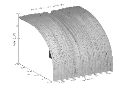
Figure 3.— Results for MCG–6-30-15: $\chi^{2}$ surfaces and confidence contours resulting from applying trial transfer function $\psi_{1}$ to the reconstructed continuum light curves and comparing with the line band light curve. Surfaces are plotted using $log_{10}(\chi^{2}-\chi^{2}_{\rm min}+1)$ as the ordinate in order to display the topography of the region near the minimum. Contours are shown the following levels: $\chi^{2}-\chi^{2}_{\rm min}=2.3,4.6,9.2,20,50,100,200$. The first three of these contours correspond to $1\sigma$, 90% and 95% for two interesting parameters and are shown in bold.

3.3. The overall time delays between bands

Figure 4.— The $f_{\rm tr}=1$ slice through the $\chi^{2}$ surface produced by folding the 2–4 keV light curve through the trial transfer function $\psi_{1}$ and comparing with the 8–15 keV light curve. Note the small (1 bin) delay between the two light curves (with the harder band lagging the softer).

By considering the $f_{\rm tr}=1$ slice through the $\chi^{2}$ surface produced with trial transfer function $\psi_{1}$, we can examine overall lags and leads between energy bands. Examining the 2–4 keV and 5–7 keV light curves for MCG–6-30-15 in this way, we find that the $\chi^{2}$ slice possesses a minimum at zero lag — i.e. we find no evidence for overall time lags or leads between the continuum and line bands down to 64 s, the bin size of the data. Performing the same procedure for the 2–4 keV and 8–15 keV light curves reveals a one bin offset in the position of the minimum (Fig. 4), indicating that the 8–15 keV light curve is delayed by $\sim$50–100 s as compared with the 2–4 keV light curve.

Figure 5.— Discrete Correlation Function (DCF; Edelson & Krolik 1988) between our 2–4 keV and 8–15 keV light curves. Note the asymmetry in the DCF which validates our detection of a $\sim 50-100{\rm\thinspace s}$ time lag between these two bands using the PRH92 method.

Lee et al. (1999b) have applied CCF methods to this RXTE dataset. By carefully comparing with simulations, they find evidence that the 7.5–10 keV band lags the lower energy bands with a phase delay of $\phi\sim 0.6$. They also find evidence that the hard band (10–20 keV) lags the softer bands with a time delay similar to that found in this work. Figure 5 shows the DCF for our 2–4 keV and 8–15 keV lightcurves (this is very similar to Fig. 17 of Lee et al. 1999b). A small time lag of 50–100 s between these two bands is evident. Thus, CCF methods and the optimal reconstruction method both suggest a time lag of 50–100 s between the 2–4 keV and 8–15 keV bands.

3.4. The meaning of an additive offset

Our fitting in Section 3.2 clearly reveals the need for an additive offset (i.e. non-zero $K$ value) between the line and continuum band light curves. In other words, the fractional variability about the mean level is less in the line band that it is in the continuum band.

The spectral analysis of Lee et al. (1999b) allows this behaviour to be understood in terms of the spectral phenomenology. Firstly, Lee et al. found that on timescales of ${\rm few}\times 10$ ksec, the iron line flux does not track the continuum flux and, instead, remains approximately constant. Secondly, it was found that there are flux correlated changes in the photon index by as much as $\Delta\Gamma\approx 0.2$ in the sense that higher flux states are softer. Both of these spectral changes will tend to reduce variability in the line band as compared with the (softer) continuum band.

4. Applications to simulations

4.1. Constructing the simulated light curves

Figure 6.— Panel (a) shows a portion of the simulated light curve described in Section 3 of the text. The simulated data possess 64 s bins, and noise is purely due to counting statistics. The squares in panel (b) show the results of applying the PRH92 reconstruction to the simulated data (using $N=3000$ simulated data points. The solid erratic line shows the ‘real’ simulated signal. Note how well the reconstruction reproduces the ‘real’ signal during times where data exists, and brackets the signal at other times.

In order to assess the significance and robustness of the above results, this section describes the application of this method to simulations. We tailor our simulation to match the RXTE observation MCG–6-30-15 as much as possible. EXOSAT showed that the high frequency fluctuations of MCG–6-30-15 possess a power spectrum of the form $f^{-1.36}$. We use this power spectrum with an additional low-frequency cutoff at $f_{c}=10^{-6}{\rm\thinspace Hz}$:

$$P(f)=\left(\frac{1}{1+(f/f_{c})}\right)^{\alpha}.$$ (23)

We then make a (noiseless) simulated continuum light curve, $F(t)$, by summing Fourier components of random phase between $f_{\rm min}=10^{-7}{\rm\thinspace Hz}$ and $f_{\rm max}=1{\rm\thinspace Hz}$, i.e.

$$F(t)=\int^{f_{\rm max}}_{f_{\rm min}}df\,P(f)\sin[2\pi\,f\,t-\phi(f)]$$ (24)

where $\phi(f)$ is a uniformly randomly distributed in the range $0$ to $2\pi$ for each distinct value of $f$.

Without loss of generality, we assume that the line band flux possesses the same mean normalization as the continuum band light curve. However, in order to mimic the situation found in Section 3 as closely as possible, we assume that there is an additive offset between the continuum band and line band light curves as well as the convolution a transfer function. In other words we compute a (noiseless) line-band light curve using the expression:

$$b(t)=(1-f)\Lambda\,a(t)+f\int_{-\infty}^{+\infty}d\tau\Psi_{1,nzl}(\tau)a(t-\tau)+K.$$ (25)

Here, $\Psi_{1,nzl}$ is the non-zero-lag component of our imposed simulated transfer function for which we use a Gaussian:

$$\Psi_{1,nzl}={\sigma}\sqrt{\frac{2}{\pi}}\exp\left(-\frac{(t-t_{0})^{2}}{2\sigma^{2}}\right)$$ (26)

where $f$ is the fraction of the continuum flux that is delayed, $t_{0}$ is the mean time delay, and $\sigma$ is the temporal standard-width of the smearing. For concreteness, we set

$$\Lambda = 0.75$$ (27)

$$f = 0.15$$ (28)

$$K = 0.85$$ (29)

$$t_{0} = 1.0\times 10^{4}{\rm\thinspace s}$$ (30)

$$\sigma = 2.0\times 10^{3}{\rm\thinspace s}.$$ (31)

This value of $f$ is approximately the fraction of the line-band flux which originates from the iron line, and hence this simulation crudely mimics the effect of iron line reverberation with a $10^{4}{\rm\thinspace s}$ time delay. Our value of $K$ is set to be similar that found for MCG–6-30-15 above.

From these ‘perfect’ noiseless light curves, we formed Possion sampled noisy light curves assuming a mean count rate of 4 cps in both the continuum and line bands, and using 64 s bins. The datagap structure of the real MCG–6-30-15 dataset was then imposed on the simulated light curves.

We now examine our realistic, simulated, data in order to assess how well we can detect the existence of the imposed lag and recover the properties of $\Psi_{1,nzl}$ using our method.

4.2. Extracting the lag from the simulations

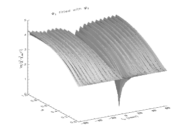
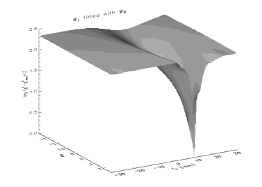
Figure 7.— Results for the simulated light curves: $\chi^{2}$ surfaces and confidence contours resulting from applying trial transfer functions $\psi_{1}$ and $\psi_{2}$ to the reconstructed continuum light curves and comparing with the line band light curve (allowing for an additive offset between the bands). Surfaces are plotted using $log_{10}(\chi^{2}-\chi^{2}_{\rm min}+1)$ as the ordinate in order to display the topography of the region near the minimum. Contours are shown the following levels: $\chi^{2}-\chi^{2}_{\rm min}=2.3,4.6,9.2,20,50,100,200$. The first three of these contours correspond to $1-\sigma$, 90% and 95% for two interesting parameters and are shown in bold. In both cases, the existence of a deep hole in $\chi^{2}$ space demonstrates that the imposed lag has been clearly detected and its parameters recovered.

We use the method of Section 2.1 and 2.2 to form an optimally reconstructed, evenly-sampled continuum lightcurve. The covariance model used is given by eqn (13) and (14) with

$$A = 2.5\,{\rm cps}$$ (32)

$$\tau_{0} = 6.23\times 10^{3}{\rm\thinspace s}$$ (33)

$$\alpha_{1} = 0.855$$ (34)

$$\alpha_{2} = 1$$ (35)

$$\langle s\rangle = 3.63\,{\rm cps}$$ (36)

A total of $N=3000$ simulated data points were used to form the reconstruction which spans a simulated observation time of 400 000 s. A portion of the simulated dataset and its reconstruction are presented in Fig. 6. Note how well the reconstruction algorithm recovers the real signal during the times with data, and brackets the real signal during other times.

Figure 7 presents the $\chi^{2}$ surfaces and confidence contours that result from passing the simulated light curves through the trial transfer functions $\psi_{1}$ and $\psi_{2}$, including minimization over any additive offset between the continuum and line band light curves. Both trial transfer functions clearly detect the imposed lag in so far as a a deep and isolated hole is present in the $\chi^{2}$ surface at approximately the right time delay, delay fraction and delay width. Note that the $f_{\rm tr}$ dimension, which has been suppressed in the $\psi_{2}$ plots, has a value of $f_{\rm tr}=0.16$ at the global minimum. This demonstrates the power of this technique for finding and characterizing subtle time lags or leads that are present in such data.

5. Discussion

In order to bring structure to the discussion that follows, we will summarize the pertinent results from this paper.

1. We clearly see reduced fractional variability in the iron line band (5–7 keV) as compared with the continuum band (2–4 keV). This is the origin of the additive offset, $K$, that was introduced in Section 3. The spectral fitting results of Lee et al. (1999b) suggests that this is due to a combination of a constant iron line flux and flux correlated changes in the photon index.

2. Our analysis finds no evidence for iron line reverberation effects. By running a number of simulations, we find that any reverberation time delays must be less than $\sim 500{\rm\thinspace s}$ or greater than $\sim 50$ ks. Together with the above result, this suggests an approximately constant iron line flux over these timescales. Thus, we can extend the work of Lee et al. (1999b) and infer a constant iron line on timescales down to $0.5$ ksec.

3. Any overall time lag between the 2–4 keV and 5–7 keV band is less than $\sim 50$ s. However, we do find that the 8–15 keV band is delayed with respect to the 2–4 keV band by 50–100 s. We can use this time delay to obtain a rough size scale for the Comptonizing cloud that is producing the hard X-rays. Assuming a coronal temperature of $\sim 100{\rm\thinspace keV}$, it takes approximately 3 inverse Compton scatterings for a photon to be boosted between the 2–4 keV and 8–15 keV bands. Thus, the mean free path of a photon is approximately 15–30 light seconds. This is a lower limit on the size of the Comptonizing region.

As we will see, this combination of facts presents problems for current models.

5.1. Simple reflection models

Initially, let us discuss these results in the light of simple X-ray reflection models (e.g. George & Fabian 1991). Assuming that variations in the primary flux are not accompanied by gross changes in geometry, we expect to observe one of two cases. Firstly, if the light crossing time of the fluorescing part of the disk is shorter than the timescale being probed by the observation, an iron line with constant equivalent width will result (i.e. the iron line flux will track the flux of the illuminating primary X-ray source). On the other hand, if the light crossing time of the fluorescing disk is greater than the timescale being probed, a constant flux line will result.

Within the context of these simple reflection models, we are forced to conclude that the light crossing time of the fluorescing region is larger than $\sim 50$ ks. Since the line is relativistically broad, most of the fluorescence occurs in the central $r\sim 20GM/c^{2}$ of the disk. Setting the light crossing time of this region to be greater than 50 ks gives a black hole mass of $M_{\rm BH}\sim 2\times 10^{8}\hbox{$\rm\thinspace M_{\odot}$}$. Given such a large black hole mass, the accretion rate must be less than 1% of the Eddington rate in order to produce the observed luminosity of $L_{\rm bol}\sim 10^{44}\hbox{${\rm\thinspace erg}{\rm\thinspace s}^{-1}\,$}$ (Reynolds et al. 1997). Furthermore, the size of the X-ray emitting blobs must be small, $r_{\rm blob}/r_{\rm disk}\sim 10^{-3}$, in order to produce the very small time delays seen between different bands. Despite being so small, these blobs must be at large distances above and below the accretion disk plane, or else one would still see iron line variability as a flaring blob illuminated the patch of disk directly beneath.

To date, there are no dynamical measurements of the black hole mass in MCG–6-30-15, and hence such a model does not explicitly contradict any data. However, there are several indirect arguments that lead us to reject the inference of a large black hole mass in MCG–6-30-15. An independent indicator of the black hole mass is possible by estimating the bulge mass of the host galaxy and then applying the bulge/hole mass relationship of Magorrian et al. (1998). The B-band luminosity of the S0-galaxy which hosts this Seyfert nucleus is approximately $m_{\rm B}=13.7$ (RC3 catalogue), and this is likely to be completely dominated by the bulge since the nucleus is heavily reddened in the B-band and the galactic disk is very weak. Using a Hubble constant of $H_{0}=65\hbox{$\hbox{${\rm\thinspace km}{\rm\thinspace s}^{-1}\,$}{\rm\thinspace Mpc}^{-1}$}$, the absolute B-band magnitude of the bulge is then $M_{\rm B}-19$. Using the standard relations (Faber et al. 1997), the bulge mass is then $M_{bulge}\sim 3\times 10^{9}\hbox{$\rm\thinspace M_{\odot}$}$. Finally, applying the Magorrian et al. (1998) scaling factor between bulge mass and black hole mass gives $M_{\rm BH}\sim 1-2\times 10^{7}\hbox{$\rm\thinspace M_{\odot}$}$, an order of magnitude smaller than the black hole mass estimate in the previous paragraph.

There are also X-ray constraints that suggest a black hole mass significantly smaller than $10^{8}\hbox{$\rm\thinspace M_{\odot}$}$. MCG–6-30-15 has exhibited large amplitude X-ray variability on timescales as short as 100 s. However, the dynamical timescale of the accretion disk where the bulk of the energy is released is $t_{\rm dyn}\sim 10^{5}(M/10^{8}\hbox{$\rm\thinspace M_{\odot}$}){\rm\thinspace s}$. Thus, if the black hole really is as massive as $M_{\rm BH}\sim 2\times 10^{8}\hbox{$\rm\thinspace M_{\odot}$}$, large amplitude variability would be occurring on timescales as short as $10^{-2}t_{\rm dyn}$. It is difficult to conceive of processes which would give such variability. The final X-ray argument against a $2\times 10^{8}\hbox{$\rm\thinspace M_{\odot}$}$ black hole in MCG–6-30-15 comes from the power spectrum derived by Lee at al. (1999b) and Nowak & Chiang (1999). By comparing the power spectral density (PSD) of MCG–6-30-15 with that of NGC 5548 and Cygnus X-1, they estimate that the black hole in MCG–6-30-15 has a mass of $M_{\rm BH}\sim 10^{6}\hbox{$\rm\thinspace M_{\odot}$}$.

5.2. More complex scenarios

Since the application of simple X-ray reflection arguments led us to deduce an unacceptably large black hole mass, we must examine alternative avenues. Indeed, the spectral fitting of Lee et al. (1999b) forces us to consider complications beyond the simple reflection picture — In their spectral fitting, they found that the Compton reflection continuum fails to show the expected correlation with the iron line equivalent width (in fact, they are anti-correlated; Lee et al. 1999b). Very similar behaviour is also seen in NGC 5548 (Chiang et al. 1999)

Ionization of the disk surface is one of the few physical phenomenon that can (partially) decouple the strength of the Compton reflection continuum from the strength of the iron line. Matt, Fabian & Ross (1993) demonstrated that the iron emission line is more sensitive to ionization effects than the general form of the Compton reflection continuum. In other words, patches of the disk with certain (surface) ionization parameters can produce a Compton reflection continuum without producing appreciable iron fluorescence.

We use this fact to construct the following simple model. Let the X-ray flux illuminating the surface layers of the accretion disk be

$$F(r)\propto F_{\rm X}r^{-\beta}.$$ (37)

A variety of X-ray source geometries give $\beta\approx 3$ at large radii, and $\beta<3$ as one approaches the innermost parts of the disk. Now, the ionization parameter of at the surface of the disk is given by

$$\xi=\frac{4\pi F(r)}{n(r)},$$ (38)

where $n(r)$ is the density of the surface layers of the disk. We suppose that $n(r)\propto r^{-\gamma}$. Hence, we have

$$\xi\propto F_{\rm X}r^{\gamma-\beta}$$ (39)

Standard disk models (Shakura & Sunyeav 1973) give $\gamma\approx 2$ at large radii, and $\gamma<2$ near the inner part of the disk. Now, suppose that there exists a critical ionization parameter $\xi_{\rm crit}$ above which there is no iron line produced. For reasonable values of $\beta$ and $\gamma$, this gives a critical radius $r_{\rm crit}$ within which no iron line is produced. The total iron line flux expected from the object is then given by

$$F_{\rm line}\propto\int^{\infty}_{r_{\rm crit}}F(r)dr,$$ (40)

which is readily manipulated to give

$$F_{\rm line}\propto F_{\rm X}^{(1-\gamma)/(\beta-\gamma)}.$$ (41)

For our canonical values of $\beta$ and $\gamma$, this gives $F_{\rm line}\propto F_{\rm X}^{-1}$. Thus, this simple model produces an iron line flux which is anti-correlated with the flux of the illuminating source. Provided a strong Compton reflection continuum can still originate from the ionized portions of the disk, this type of picture may explain the spectral behavior that we observe.

One simple prediction of this model is that the velocity width of the line profile gets smaller as the continuum flux increases (due to an outward migration in the inner radius of the line emitting region). Of course, the toy model presented above only captures the crudest aspects of the problem. Fully self-consistent ionized reflection models must be calculated (taking into account the vertical structure of the disk; e.g. see Nayakshin, Kazanas & Kallman 1999) and compared with the data in order to test whether the picture sketched here is reasonable or not.

Even if global, flux-correlated changes in the ionization of the disk surface are responsible for the observed spectral changes, we would still expect reverberation signatures on short timescales. We have set upper limits of $\sim 500$ s on the timescale of any reverberation delay. If the black hole mass is $M_{\rm BH}\sim 1\times 10^{7}\hbox{$\rm\thinspace M_{\odot}$}$, the light crossing time of the iron line producing region is $\sim 2000$ s, and hence we need to infer a disk-hugging corona (with $h/r\sim 0.3$) in order to be compatible with the reverberation limits. If, instead, the black hole is $M_{\rm BH}\sim 1\times 10^{6}\hbox{$\rm\thinspace M_{\odot}$}$, the light crossing time of the entire line producing region is only $200{\rm\thinspace s}$ and so the X-ray source geometry is unconstrained by our reverberation limits. The corresponding Eddington ratios are $\sim 10\%$ and $\sim 100\%$ for black hole masses of $10^{7}\hbox{$\rm\thinspace M_{\odot}$}$ and $10^{6}\hbox{$\rm\thinspace M_{\odot}$}$ respectively.

6. Conclusions

In this paper, we have used an interpolation method based upon that of PRH92 to search for temporal lags and leads between the 2–4 keV, 5–7 keV and 8–15 keV bands in a long RXTE observation of the bright Seyfert 1 galaxy MCG–6-30-15. In essence, we use the PRH92 method to compute an optimal reconstruction of the 2–4 keV light curve in which the datagaps are interpolated across. We then fold this reconstructed light curve through trial transfer functions and compare with data from the other bands in a $\chi^{2}$ sense.

Our search for lags and leads was tailored to find reverberation effects in the iron line which is thought to originate from the innermost regions of the black hole accretion disk. We find no evidence for any reverberation, and rule out reverberation delays in the range $0.5-50$ ksec. We can extend the conclusions of Lee et al. (1999b), and infer that the iron line possesses a constant flux on timescales on timescales as short as 500 s. We also find that the hard band (8–15 keV) is delayed by 50–100 s relative to the 2–4 keV band.

We attempt to put these various results together into a coherent picture for this object. The constancy of the iron line flux leads one to consider large black hole masses (in excess of $10^{8}\hbox{$\rm\thinspace M_{\odot}$}$). However, such a large mass is found to be unacceptable from the standpoint of both X-ray variability constraints, and constraints based on the mass of the galactic bulge. Indeed, using the bulge/hole scaling factor of Magorrian et al. (1998), we estimate that the hole has a mass of $M_{\rm BH}\sim 1-2\times 10^{7}\hbox{$\rm\thinspace M_{\odot}$}$. Given that this is a more reasonable mass estimate, some mechanism beyond the simple X-ray reflection model must be invoked to explain the temporal variability of the iron line and Compton reflection continuum. We suggest that flux correlated changes in the average ionization state of the surface layers of the accretion disk may be such a mechanism. While we support this suggestion with a toy model, the plausibility if this suggestion can only be assessed once detailed modeling has been performed.

References

- (1) Chiang J. et al., 1999, ApJ, submitted.
- (2) Dabrowski Y., Fabian A. C., Iwasawa K., Lasenby A. N., Reynolds C. S., 1997, MNRAS, 288, L11
- (3) Edelson R. A., Krolik J. H., 1988, ApJ, 333, 646
- (4) Faber S. M. et al., 1997, AJ, 114, 1771
- (5) Fabian A. C., Rees M. J., Stellar L., White N. E., 1989, MNRAS, 238, 729
- (6) Guilbert P. W., Rees M. J., 1988, MNRAS, 233, 475
- (7) Horne K., Welsh W. F., Peterson B. M., 1991, ApJ, 367, L5
- (8) Iwasawa I. et al.,1996, MNRAS, 282, 1038
- (9) Krolik J. H., Horne K., Kallman T. R., Malkan M. A., Edelson R. A., Kriss G. A., 1991, ApJ, 371, 541
- (10) Lee J. C., Fabian A. C., Brandt W. N., Reynolds C. S., Iwasawa K., 1999a, MNRAS, in press
- (11) Lee J. C. et al., 1999b, in preparation
- (12) Lee J. C., Fabian A. C., Reynolds C. S., Iwasawa K., Brandt W. N., 1998, MNRAS, 300, 583.
- (13) Lightman A. P., White T. R., 1988, ApJ, 335, 57
- (14) Magorrian J. et al., 1998, AJ, 115, 2285
- (15) Matsuoka M., Piro L., Yamauchi M., Murakami T., 1990, ApJ, 361, 440
- (16) Matt G., Fabian A. C., Ross R. R., 1993, MNRAS, 262, 179
- (17) Nandra K., Pounds K. A., Stewart G. C., 1990, MNRAS, 242, 660
- (18) Nandra K., Pounds K. A., Stewart G. C., Fabian A. C., Rees M. J., 1989, MNRAS, 236, L39
- (19) Nandra K., George I. M., Mushotzky R. F., Turner T. J., Yaqoob T., 1997, ApJ, 477, 602
- (20) Nayakshin S.,Kazanas D., Kallman T. R., 1999, ApJ submitted (astro-ph/9909359).
- (21) Nowak M. A., Chiang J., 1999, ApJL, subimtted
- (22) Nowak M. A., Vaughan B. A., Wilms J., Dove J., Begelman M. C., 1999, ApJ, 510, 874
- (23) Press W. H., Rybicki G. B., Hewitt J. N., 1992, ApJ, 385, 404 (PRH92)
- (24) Reynolds C. S., 1999, in High Energy Processes in Accreting Black Holes, eds J. Poutanen, R. Svennson, p.178, ASP Conf. Ser. vol. 161.
- (25) Reynolds C. S., Begelman M. C., 1997, ApJ, 488, 109
- (26) Reynolds C. S., Young A. J., Begelman M. C., Fabian A. C., 1999, ApJ, 514, 164
- (27) Reynolds C. S., Ward M. J., Fabian A. C., Celotti A., 1997, MNRAS, 291, 403
- (28) Reynolds C. S., Fabian A. C., Nandra K., Inoue H., Kunieda H., Iwasawa K., 1995, MNRAS, 277, 901
- (29) Shakura N. I., Sunyaev R. A., 1973, A&A, 24, 337
- (30) Stella L., 1990, Nat., 375, 659
- (31) Tanaka Y. et al., 1995, Nat, 375, 659
- (32) Young A. J., Ross R. R., Fabian A. C., 1998, MNRAS, 300, L11