Gravitational Waves from Long-Duration Simulations of the Dynamical Bar Instability

Abstract

Compact astrophysical objects that rotate rapidly may encounter the dynamical “bar instability.” The bar-like deformation induced by this rotational instability causes the object to become a potentially strong source of gravitational radiation. We have carried out a set of long-duration simulations of the bar instability with two Eulerian hydrodynamics codes. Our results indicate that the remnant of this instability is a persistent bar-like structure that emits a long-lived gravitational radiation signal.

PACS numbers: 04.30.Db, 04.40.Dg, 95.30.Lz, 97.60.-s

I Introduction

The direct detection of gravitational radiation presents one of the greatest scientific challenges of our day. With interferometers such as LIGO, VIRGO, GEO, and TAMA [2] expected to be operating in the next few years, and a new generation of spherical resonant mass detectors under study [3, 4], the calculation of the signals expected from various astrophysical sources has a high priority. Accurate calculations of the waveforms are needed to enable both the detection and identification of sources [5]. In particular, short duration bursts are expected to be more difficult to detect than longer-lived signals.

One interesting class of sources includes rapidly rotating compact objects that develop the rotationally-induced “bar instability”. This instability derives its name from the bar-like deformation it induces. The resultant object is potentially a strong source of gravitational radiation because of its highly nonaxisymmetric structure. Examples of compact astrophysical objects that may rotate rapidly enough to encounter this instability include stellar cores that have expended their nuclear fuel and are prevented from undergoing further collapse by centrifugal forces [6, 7, 8, 9, 10, 11]; a neutron star spun up by accretion from a binary companion [12, 13]; and the remnant of a compact binary merger [14, 15].

Such global rotational instabilities in fluids arise from nonaxisymmetric modes $e^{\pm im\varphi}$, where $m=2$ is known as the “bar mode”. It is convenient to parametrize them by

$$\beta=T_{\rm rot}/|W|,$$ (1)

where $T_{\rm rot}$ is the rotational kinetic energy and $W$ is the gravitational potential energy [16, 17, 18]. In this paper, we focus on the dynamical bar instability, which is driven by Newtonian hydrodynamics and gravity, and is expected to be the fastest growing mode. It operates for fairly large values of the stability parameter $\beta>\beta_{\rm d}$ and develops on a timescale on the order of the rotation period of the object. For the uniform density, incompressible, uniformly rotating Maclaurin spheroids, $\beta_{\rm d}\approx 0.27$. In the case of differentially rotating fluids with a polytropic equation of state, the $m=2$ dynamical stability limit $\beta_{\rm d}\approx 0.27$ has been numerically determined to be valid for initial angular momentum distributions that are similar to those of Maclaurin spheroids [17, 18, 19, 20]; see also [21, 22]. (We note that when $\beta$ is greater than some critical value $\beta_{\rm s}<\beta_{\rm d}$, a secular instability can arise from dissipative processes such as gravitational radiation reaction and viscosity. When this instability arises, it develops on the timescale of the relevant dissipative mechanism, which can be several rotation periods or longer [13]. In recent years, much work has also been carried out on various other modes in rotating relativistic stars as detectable sources of gravitational radiation; see [23] for a review and references.)

The first numerical simulations of the dynamical bar instability were carried out by Tohline, Durisen, and McCollough (TDM; [24]) in the context of star formation. Using a polytropic equation of state,

$$P=K\rho^{\Gamma}=K\rho^{1+1/N},$$ (2)

with polytropic index $N=1.5$, they evolved differentially rotating axisymmetric models with a 3-D Eulerian hydrodynamics code, or hydrocode, in Newtonian gravity. In all models with initial $\beta\geq 0.30$, the $m=2$ mode grew to nonlinear amplitudes and a two-armed spiral pattern was produced as mass and angular momentum were shed from the ends of the bar. Numerous other simulations have confirmed this basic scenario for the evolution of the bar mode into the nonlinear regime; see Sec. II for references and further discussion.

More recently, these techniques have been extended to the context of rapidly rotating, compact objects in the Newtonian regime, with the gravitational waves calculated in the quadrupole limit. This is a reasonable first approximation for an object, such as a centrifugally-hung stellar core with a density intermediate between that of white dwarfs and neutron stars, with initial mass $M=1.4{\rm M}_{\odot}$ and radius $R\mathrel{\hbox{\hbox to0.0pt{\hbox{\lower 4.0pt\hbox{$\sim$}}\hss}\hbox{$>$}}}100$ km, and hence $GM/Rc^{2}\mathrel{\hbox{\hbox to0.0pt{\hbox{\lower 4.0pt\hbox{$\sim$}}\hss}\hbox{$<$}}}0.02$. Centrella and collaborators used both smooth particle hydrodynamics (SPH) and Eulerian finite difference hydrodynamics to evolve the bar instability in a model with $N=1.5$ [25, 26]. In all of their runs the gravitational wave signal was a relatively short duration burst lasting for several bar rotation periods, and the system evolved to a nearly axisymmetric central core surrounded by a flattened, disk-like halo. New [27] carried out a similar study, with an improved version of Tohline’s Eulerian code [28]. Her simulation employed a symmetry condition that only permitted the growth of even modes $m$; see Sec. II. This simulation produced a final state with a persistent bar-like core, which yielded a gravitational wave signal of much longer duration than that found by Centrella and collaborators.

Given the requirements of reliable waveforms for the detection and identification of sources, it is important to resolve this issue of the late-time gravitational wave signal from the dynamical bar instability. To this end, we have carried out a set of long-duration runs using the two Eulerian codes employed by New and by Centrella in their earlier work, and have made a detailed study of the resulting models. In Section II we review previous numerical studies of the dynamical bar instability, highlighting the various assumptions and restrictions used by different authors. The numerical techniques we used are discussed in Sec. III. In Sec. IV we present our simulations and analyze the results. A discussion of these results follows in Sec. V. Finally, the Appendix contains additional information about the two hydrocodes used in this work.

II Previous Numerical Studies

As mentioned above, the work of TDM [24] set the stage for subsequent numerical calculations of the dynamical bar instability. Their initial models consisted of differentially rotating, axisymmetric equilibrium spheroids with a Maclaurin rotation law for the angular momentum distribution. The Maclaurin law produces rigid rotation when it is applied to an incompressible ($N=0$) fluid; when it is used in a polytrope, it produces differential rotation [16]. After small amplitude random perturbations were applied to the density, each model was evolved into the nonlinear regime using a 3-D Eulerian hydrocode with Newtonian gravity. This hydrocode solved the mass continuity and Euler equations in cylindrical coordinates $(\varpi,z,\varphi)$; the resulting evolutions were adiabatic and maintained the same polytropic equation of state, Eq. (2).

TDM used equatorial symmetry and “$\pi$-symmetry” in their simulations. Equatorial symmetry is a reflection symmetry through the equatorial plane $z=0$. The $\pi$-symmetry condition imposes periodic boundary conditions at angles $\varphi=\pi$ and $\varphi=2\pi$; thus, physical variables are the same in the interval $0\leq\varphi<\pi$ as they are in $\pi\leq\varphi<2\pi$. It is computationally advantageous to impose an equatorial- and/or $\pi-$ symmetry condition on such a simulation because, by doing so, half as many computational grid zones are required in order to achieve a given spatial resolution in the vertical and/or azimuthal coordinate directions, respectively. It was also physically reasonable for TDM to adopt both of these symmetry conditions because the eigenfunction (a pure, $m=2$ barmode) to which their models were expected to be initially unstable had both equatorial and $\pi-$symmetry [24, 29]. As we discuss more fully below, ultimately one would like to remove these computational constraints in order to test whether or not the physical outcome is sensitive to them.

The first work to address the late-time development of the bar instability was published by Durisen, Gingold, Tohline, and Boss [30], who ran simulations with $\beta=0.33$ and $\beta=0.38$ for $N=1.5$ polytropes. They used three different 3-D hydrocodes: Tohline’s Eulerian code as used in TDM, another Eulerian code developed in spherical coordinates by Boss, and an SPH code developed by Gingold. Boss’s code also enforced equatorial- and $\pi$-symmetries but, being gridless, Gingold’s SPH code imposed neither of these symmetries. However, the SPH simulations were limited to a very small number of particles, $N_{\rm p}=2000$. The results produced by these three separate simulation codes were qualitatively similar. For example, at early times all simulations showed evidence of the development of a bar-like pattern instability, consistent with the results of TDM and the predictions of linear perturbative analysis [16, 24, 29, 22]. Peturbative analysis says this instability is the result of the growth of a coherent bar-like wave that propagates around the system with a well-defined pattern speed, while material moves differentially through that pattern. At subsequent times in the simulations, the barmode distortion developed into a two-armed, trailing spiral pattern as described by TDM; when the spiral pattern reached a nonlinear amplitude, some relatively high specific angular momentum material was expelled in the equatorial plane of each system; and the primary structure that remained at the end of each simulation was a dynamically stable, centrally condensed object exhibiting a value of $\beta<\beta_{\rm d}$. But there were significant quantitative differences among the various evolutions presented by Durisen et al. For example, the simulations produced central remnants that had different total masses and exhibited different degrees of nonaxisymmetric distortion. This disagreement signified, in part, that the simulation techniques being used were rather primitive and, in part, that the available computing resources did not permit the simulations to be carried out with adequate spatial resolution.

Williams and Tohline subsequently carried out an investigation of the dynamical barmode instability in models with different polytropic indices. Using the TDM code with $\pi$-symmetry and an improved azimuthal grid resolution, they first considered models with initial $\beta=0.31$ and $N=0.8,1.0,1.3,1.5$, and $1.8$, and focused their analysis on the measurement of barmode growth rates and pattern speeds in the linear-amplitude growth regime [29]. The runs with $N=0.8$ and $N=1.8$ were then extended to later times through the development of nonlinear-amplitude nonaxisymmetric structures and yielded a rotating triaxial central remnant [31]. Williams and Tohline noted that such a configuration would be of interest when viewed in the context of compact stellar objects because “its existence would presumably be discernable from the spectrum of any emitted gravity wave radiation,” but they did not derive such a spectrum from their models.

Houser, Centrella, and Smith [25, 26] were the next to carry out 3-D simulations of the dynamical bar instability for the case $N=1.5$ and initial $\beta\approx.30$, this time in the context of rapidly rotating stellar cores. Using both an SPH and an Eulerian code, they considered the matter to be a perfect fluid with equation of state

$$P=(\Gamma-1)\rho\epsilon,$$ (3)

where $\epsilon$ is the specific internal energy, and solved an equation for the internal energy. Using artificial viscosity, they could account for the energy generation by shocks that occurs when the spiral arms form and deflect the streamlines of the supersonically moving fluid. Routines were added to calculate the gravitational waveforms and luminosities in the quadrupole approximation. The SPH code (developed from TREESPH; see [32]) imposed no symmetry restrictions and was run with up to $N_{\rm p}=32,914$ particles. Their Eulerian code, written in cylindrical coordinates, imposed symmetry through the equatorial plane but not $\pi$-symmetry [33]. Overall, their simulations produced nearly axisymmetric central remnants at late times.

Houser and Centrella [34] carried out additional SPH simulations with $N=1.5,1.0,$ and $0.5$, and initial $\beta\approx 0.30$ using improved initial models with $N_{\rm p}\approx 16,000$ particles. As before, the $N=1.5$ case resulted in an almost axisymmetric central remnant and a correspondingly short burst of gravitational radiation. The runs with $N=1.0$ and $N=0.5$ underwent additional episodes of spiral arm ejection, with the number of episodes increasing as $N$ decreased; such behavior was also observed by Williams and Tohline [31]. This resulted in longer-lived nonaxisymmetric structure in the central remnants, accompanied by longer duration gravitational waveforms as the models grew stiffer (i.e., as $N$ was decreased). Note that the relatively small number of particles present in the SPH simulations of Centrella and collaborators, accompanied by the velocity dispersion in their initial models, may make it difficult for models with softer equations of state (larger $N$) to maintain long-lived nonaxisymmetric structures.

New [27] used an improved version of Tohline’s code [28] to study the $N=1.5$, $\beta=0.30$ case. This code solves an energy equation and incorporates artificial viscosity to handle the shocks. She added a routine to calculate the gravitational radiation in the quadrupole limit. Her simulation, which imposed both equatorial and $\pi-$symmetries, produced a persistent bar structure and a long-duration gravitational waveform.

All of the studies mentioned above in this section started from initially axisymmetric models with the same radial distribution of specific angular momentum as in a Maclaurin spheroid. Pickett, Durisen, and Davis [21] studied the instabilities that result in an $N=1.5$ polytrope, when the angular momentum distribution is varied. They used a (different) updated version of Tohline’s code with neither equatorial plane symmetry nor $\pi$-symmetry imposed; all their evolutions were adiabatic. Using the Maclaurin rotation law, they evolved a model with initial $\beta=0.327$ to late times, and obtained a bar-shaped central remnant.

Recently Imamura, Durisen, and Pickett [35] have performed additional adiabatic simulations of dynamical instabilities in $N=1.5$ and $2.5$ polytropes with the Maclaurin rotation law, using the same hydrodynamics code used in [21]. They focused on comparing the early phases of nonlinear mode growth in their runs with the predictions of quasi-linear approximations. Their high resolution simulations of $N=1.5$ polytropes with $\beta=0.304$ and $0.327$ both resulted in bar-like endstates.

The properties and outcomes of the long duration bar mode runs with $N=1.5$ and $N=1.8$ are summarized in Table I for convenience. All of the times reported in Table I are given in units of $t_{\rm c}$, where $t_{\rm c}$ is defined as one central initial rotation period (cirp). When surveying the information catalogued in Table I, one should keep in mind that the identified “final” state has been reported at different evolutionary times in the various references. As this table emphasizes, over the fifteen years that have passed since the original Durisen et al. comparison paper [30], there remain significant quantitative differences among the results of various published simulations of the bar mode instability. In particular, as indicated by our comments under the “remarks” column, these previous simulations do not clearly indicate whether or not the end product of the evolution should be a central, steady-state structure that has a bar-like geometry.

III Numerical Techniques

A Initial Axisymmetric Equilibria

The new simulations of the dynamical bar instability presented here begin with rotating spheroidal models above the Maclaurin stability limit, $\beta>\beta_{d}$, constructed in hydrostatic equilibrium. For fluids rotating about the $z-$axis with angular velocity $\Omega=\Omega(\varpi)$, where $\varpi$ is the distance from the rotation axis, the equations of motion reduce to the equation of hydrostatic equilibrium,

$$\frac{1}{\rho}\nabla P+\nabla\Phi+h_{0}^{2}\nabla\Psi=0,$$ (4)

where $\Psi(\varpi)=-1/h_{0}^{2}\int\Omega^{2}(\varpi)\varpi\;d\varpi$ is the centrifugal potential and $h_{0}$ is a constant. The gravitational potential $\Phi$ is a solution to Poisson’s equation,

$$\nabla^{2}\Phi=4\pi G\rho.$$ (5)

The initial models for the runs discussed in this paper were constructed using Hachisu’s Self-Consistent Field (HSCF; [36]; see also [27]) technique, which is a grid-based iterative method. To facilitate treatment of the boundary conditions, it uses the integral form of the hydrostatic equilibrium condition, Eq. (4). This gives

$$H+\Phi+h_{0}^{2}\Psi=C,$$ (6)

where $H\equiv\int\rho^{-1}dP$ is the enthalpy of the fluid and $C$ is a constant determined by the boundary conditions. The models are computed on a uniformly-spaced $(\varpi,z)$ grid. The method requires an equation of state $P=P(\rho)$. For the polytropic relation in Eq. (2), the enthalpy takes the form

$$H=(1+N)K\rho^{1/N}.$$ (7)

For purposes of comparison with earlier work, we follow Bodenheimer and Ostriker [37] and adopt a specific angular momentum profile that is the same function of cylindrical mass as a Maclaurin spheroid, namely,

$$\Omega(\varpi)=h_{0}\left[1-(1-m(\varpi)/M)^{2/3}\right]\varpi^{-2},$$ (8)

where $M$ is the total mass of the system, $m(\varpi)$ is the mass interior to cylindrical radius $\varpi$, the constant $h_{0}\equiv 5J/2M$, and $J$ is the total angular momentum. Hence, the centrifugal potential is,

$$\Psi(\varpi)=-\int\left[1-(1-m(\varpi)/M)^{2/3}\right]^{2}\varpi^{-3}d\varpi.$$ (9)

Because the angular velocity is assumed initially to be only a function of $\varpi$, Lichtenstein’s theorem implies that the configuration will have reflection symmetry through the equatorial plane [16].

The HSCF method requires that two boundary points, $A$ and $B$, on the surface of the model be selected [36]. For spheroids, point $A$ is set along $\varpi$ at the equatorial radius, $\varpi(A)=\varpi_{\rm E}$, and point $B$ is set on the $z-$axis at the polar radius, $z(B)=z_{\rm P}$. The axis ratio $z_{\rm P}/\varpi_{\rm E}$ is given as an input parameter; varying it produces equilibrium models with different values of $\beta$. Points $A$ and $B$ set the boundary conditions for the solution of Eq. (6). Since $\rho$, $P$, and therefore $H$ vanish on the surface of the polytropic fluid, we have

$$H(A)=0=C-\Phi(A)-h_{0}^{2}\Psi(A),$$ (11)

$$H(B)=0=C-\Phi(B)-h_{0}^{2}\Psi(B).$$ (12)

Once $\Phi$ and $\Psi$ are known, Eqs. (III A) can be solved for the constants $C$ and $h_{0}^{2}$.

The HSCF iteration process begins with an initial guess for $\rho(\varpi,z)$, which also specifies the mass enclosed within each cylindrical radius $m(\varpi)$. Given $\rho$, the gravitational potential $\Phi(\varpi,z)$ is determined by solving Poisson’s equation, Eq. (5); see Ref.[38] for details. Given $m(\varpi)$, the centrifugal potential $\Psi(\varpi)$ is determined using Eq. (9). Then, $C$ and $h_{0}^{2}$ are found from the boundary conditions, Eqs. (III A), and the enthalpy $H$ is computed from Eq. (6). Finally, a new density distribution is calculated from $H$ by inverting Eq. (7); this is used as input for the next iteration cycle. The process is repeated until fractional changes in $C$ and $h_{0}^{2}$ and the maximum fractional change in $H$ between two successive iteration steps are less than some threshold (in this work, $10^{-8}$). The virial error $VE$ provides a measure of how well the energy is balanced, and thus is indicative of the quality of the resulting equilibrium configuration. It is defined by [36]

$$VE=2T+W+3\int PdV,$$ (13)

where $T$ is the total kinetic energy, and $V$ is the volume of the model. The $VE$s for the models used here are $\sim 10^{-3}$.

B 3-D Hydrodynamics Codes

The simulations presented in this paper were carried out using two hydrocodes that employ Eulerian finite-differencing techniques to solve the equations of hydrodynamics coupled to Newtonian gravity. The ${\cal D}$ (Drexel) hydrocode is the same one that was used by Smith, Houser, and Centrella [26] in their studies of the bar instability, whereas the ${\cal L}$ (LSU) hydrocode is the one that was used by New and Tohline [27, 39]. In this section we briefly describe these codes, highlighting differences between them that we believe to be most relevant to the analysis and discussion of our results. Further details on the ${\cal D}$ and ${\cal L}$ hydrocodes may be found in the Appendix.

Both 3-D hydrocodes are written on uniform grids in cylindrical coordinates $(\varpi,z,\varphi)$. The ${\cal D}$ code assumes equatorial plane symmetry. The ${\cal L}$ hydrocode allows the use of both equatorial and $\pi$-symmetries, as discussed in Sec. II. Both codes handle the transport terms using similar monotonic advection schemes that are second-order accurate in space, and impose the same outflow boundary conditions on the edges of the grid. The ${\cal D}$ and ${\cal L}$ codes both solve energy equations, using the perfect fluid relation of Eq. (3) to calculate the gas pressure and artificial viscosity to handle shocks. Finally, both codes solve Poisson’s equation, Eq. (5), for the Newtonian gravitational potential $\Phi$ with boundary conditions on the edges of the grid specified in terms of spherical harmonics.

Eulerian codes typically require that the mass density in a grid zone never be zero, and thus fill the “vacuum” regions with a fluid having some small density, $\rho_{\rm low}$. To facilitate the comparison of results in this paper, both codes impose essentially the same conditions in the “vaccum” regions. The density is set to $\rho=\rho_{\rm low}$ if the density drops below $\rho_{\rm low}$ in a zone. The specific internal energy is similarly limited by $\epsilon\geq\epsilon_{\rm low}$, where Eqs. (2) and (3) give $\epsilon_{\rm low}=K\rho_{\rm low}^{\Gamma-1}/(\Gamma-1)$ and $K$ is the polytropic constant of the initial model. In addition, the velocities in the low density zones must be limited to prevent them from becoming too large and thereby requiring very small timesteps through the Courant criterion [40]. The velocities are limited when $\rho\leq\rho_{lim}=10^{3}\rho_{low}$. Specifically, in cells where $\rho\leq\rho_{lim}$, $v_{\varpi}$ and $v_{z}$ are set to the value $0.5c_{s,max}$, if they exceed $c_{s,max}$. Here, $c_{s,max}$ is the globally maximum sound speed. Additionally, $v_{\varphi}$ is set to zero in cells where $\rho\leq\rho_{lim}$ and $v_{\varphi}/\varpi>\Omega_{lim}$. Here, $\Omega_{lim}=\Omega_{0}/4$, where $\Omega_{0}$ is the central rotation speed of the initial model.

The codes do have a number of differences. The most important of these is that, as discussed in the Appendix, the hydrodynamical equations in the ${\cal L}$ code are written in flux-conservative form whereas in the ${\cal D}$ code they are not. The accuracy of the ${\cal L}$ code is second-order in both space and time [61, 62, 63]. However, while the ${\cal D}$ code is spatially second-order accurate, the accuracy of its time evolution scheme is between first and second orders [53, 40]. Finally, the ${\cal D}$ code was written in Fortran 77 and optimized to run on Cray vector computers such as the C90 and T90 in single-processor mode. These machines use 64-bit words in single precision, which allows the use of very low densities in the vacuum region, typically $\rho_{\rm low}=10^{-10}$. The ${\cal L}$ code was developed for the parallel MasPar MP-1 computer, and was written in MasPar Fortran, which is MasPar’s version of Fortran 90. The MasPar computers use 32-bit words in single precision, and the ${\cal L}$ code uses $\rho_{\rm low}=10^{-7}$ in the vacuum regions.

IV Analysis of Results

A Properties of the Models

The initial axisymmetric equililbrium models used for the simulations presented in this paper were computed with the HSCF method [36] as described in Sec. III A. Specifying an axis ratio $z_{\rm P}/\varpi_{\rm E}=0.208$, polytropic index $N=1.5$, and the Maclaurin rotation law, Eq. (9), yields a model with $\beta=0.298>\beta_{\rm d}$. Models with two different resolutions were constructed for this work. The lower resolution model was computed on a grid with $N_{\varpi}=64$ radial and $N_{z}=64$ axial zones; its equatorial radius extends out to zone $j=26$ and its polar radius to zone $k=7$. The higher resolution model was computed on a grid with $N_{\varpi}=N_{z}=128$; its equatorial radius extending out to zone $j=50$ and its polar radius to zone $k=12$. (Note that $\varpi=0$ in radial zone $j=2$ and $z=0$ in vertical zone $k=2$.) The computations of both models required 21 iterations. The $64\times 64$ model had a virial error $VE=2.69\times 10^{-3}$, as defined in Eq. (13); for the $128\times 128$ model, $VE=7.52\times 10^{-4}$. Density contours of this model in the $x-z$ plane are shown in Fig. 1 and plots of the angular velocity $\Omega(\varpi)$ (cf. Eq. (8)) and equatorial plane density profile $\rho(\varpi,0)$ are given in Fig. 2. We have normalized the equatorial radius and central density to unity, $\varpi_{\rm E}=1$ and $\rho_{\rm C}=1$.

To prepare the initial data for evolution with a hydrocode, the 2-D model is swept around in the azimuthal direction to create a 3-D axisymmetric model. Random perturbations are then imposed on the density to trigger the instability when the evolutions are run. Following TDM [24], we set

$$\rho(\varpi,z,\varphi)=\rho_{\rm EQ}[1+a_{0}f(\varpi,z,\varphi)],$$ (14)

where $\rho_{\rm EQ}$ is the density calculated with the HSCF code, $a_{0}=10^{-2}$, and $-1\leq f\leq+1$ is a random number.

The perturbed initial models were then evolved with the hydrocode. Note that the models were initially centered on the origin. All calculations used equatorial plane symmetry. Two simulations were performed with the ${\cal D}$ code. Model D1 had $N_{\varpi}=N_{z}=N_{\varphi}=64$ zones while model D2 had twice the angular resolution, $N_{\varphi}=128$; neither model used $\pi$-symmetry. Models D1 and D2 both used the density $\rho_{\rm low}=10^{-10}$ in the “vacuum” regions. Three simulations were performed with the ${\cal L}$ code. Model L1 was run without $\pi$-symmetry and used the same resolution as model D2; for comparison, model L2 was run with $\pi$-symmetry and $N_{\varphi}=64$ and thus had the same angular zone size $\Delta\varphi$ as model L1. Finally, model L3 was run without $\pi$-symmetry and used twice the radial and axial resolution, $N_{\varpi}=N_{z}=N_{\varphi}=128$. The models run with the ${\cal L}$ code all used $\rho_{\rm low}=10^{-7}$. Some basic properties of these models are summarized in the first five columns of Table II for convenience.

B Dynamical Evolutions

All the models give similar results for the initial growth of the instability and its development into the nonlinear regime. An initially axisymmetric system develops bar-shaped structure as the $m=2$ mode grows to nonlinear amplitude (cf. Sec. IV C, [35]). A pattern of trailing spiral arms is formed as mass and angular momentum are shed from the ends of the rotating bar. After the bar reaches its maximum elongation, it recontracts somewhat towards a more axisymmetric shape. All the runs displayed these basic characteristics, which are illustrated in Fig. 3 using data from model L3. Time is measured in units of $t_{\rm D}$, where

$$t_{\rm D}\equiv\left(\frac{R_{\rm E}^{3}}{GM}\right)^{1/2}$$ (15)

is the dynamical time for a sphere of mass $M$ having the same radius as the initial equatorial radius of the model, $R_{\rm E}=\varpi_{\rm E}$.

Significant differences in the models arise in the next stage of the evolution, shown in Figs. 4 and 5. Since the models go unstable at slightly different times, they encounter the various phases of the instability at somewhat different intervals; the frames in these figures are labeled with the time measured from the initial moment in each model. Frames (a-c) of Fig. 4 show that the central regions of model D1 appear to undergo a very slight re-expansion to a weak bar. After another $\sim 1-2$ bar rotation periods this weak bar disappears, leaving behind a nearly axisymmetric remnant that is somewhat displaced from the center of the grid. In model D2 the central bar re-expands more strongly, although not to the extent of its previous maximum elongation. After another $\sim 1-2$ bar rotation periods, the model evolves toward a nearly axisymmetric remnant, which is offset from the center of the grid; see frames (d-f) of Fig. 4. Similar behavior is seen in model L1, although the second bar elongation phase is stronger and lasts somewhat longer; representative density contours are shown in frames (a-c) of Fig. 5. The higher resolution model L3, shown in frames (d-f) of Fig. 5, also re-expanded to a fairly strong bar, which underwent two additional episodes of contraction and expansion. The remnant in model L3 remained bar-like in shape for $>4$ bar rotation periods, but eventually it also decayed and settled into a nearly axisymmetric remnant as it moved off the center of the grid. In contrast, model L2 (which was run with $\pi$-symmetry) retained a fairly strong bar for many ($>8$) bar rotation periods. This model was run for a longer time than any of the others and experienced $\sim 5$ episodes of contraction and expansion. At the end of the simulation, model L2 still had a strong bar centered on the origin; see frames (g-i) of Fig. 5.

As is illustrated in Fig. 6, for all five model evolutions each episode of expansion and contraction of the bar is mirrored in the time-evolution of the stability parameter $\beta=T_{\rm rot}/|W|$. As the bar develops and expands, $\beta$ drops and reaches a local minimum when the bar is at its maximum elongation. Then $\beta$ rises to a local maximum as the central regions recontract. This behavior occurs because $T_{\rm rot}\propto I\omega^{2}\propto J^{2}/I$. Hence, as the bar elongates its moment of inertia $I$ increases which, assuming its angular momentum is approximately conserved, reduces the rotational kinetic energy $T_{\rm rot}$. Each subsequent episode of bar re-expansion can also be associated with a local minimum in the global parameter $\beta$.

As has been illustrated by Figs. 4 and 5, in each simulation except model L2, the “final” remnant appears to have moved off of the center of the grid. In each case this displacement is associated with measurable motion of the center-of-mass of the system (such center-of-mass motion was also seen in some of the simulations in [35]). Fig. 7 shows the position of the system center-of-mass $R_{\rm CM}=[X_{\rm CM}^{2}+Y_{\rm CM}^{2}]^{1/2}$ as a function of time for each of the four affected models. (Note that $Z_{\rm CM}=0$ at all times in all of our simulations since they all employ equatorial plane symmetry.) In runs D1 and D2, the center-of-mass begins to move rather abruptly at a time $t/t_{\rm D}\sim 20$, then after moving to a location $\log(R_{\rm CM})\sim-0.5$ (D1) and $\sim-0.7$ (D2), the center-of-mass motion slows considerably. Because both models have radial zones of size $\Delta\varpi\sim 0.04$, this location corresponds to approximately $8$ and $5$ radial grid zones, respectively, or in terms of the initial equatorial radius of the model, $\sim\frac{1}{3}\varpi_{\rm E}$ and $\sim\frac{1}{5}\varpi_{\rm E}$, respectively. For models L1 and L3, the center-of-mass motion does not appear to level off, as seen in Fig. 7(b). Notice that the center-of-mass moves farthest from the center of the grid in model L1, which has the same resolution as D2, and that the onset of this motion is significantly delayed when the radial resolution is doubled in model L3.

Since these simulations all have Newtonian gravitational fields and the systems are assumed to be isolated from the external environment, in each case the center-of-mass should remain fixed at the origin if the total mass of the system remains confined within the boundaries of the computational grid (i.e., if the system remains isolated from its environment) and if the equations governing the dynamics of an isolated system are being properly integrated forward in time. Although some ($<5\%$) mass (and associated linear and angular momentum) does flow radially off the grid, this mass loss does not appear to be large or asymmetric enough to account for the center-of-mass motion. We have verified this by running a simulation (not presented in detail in this manuscript) with the same resolution as model L1 but with an expanded grid ($N_{\varpi}=N_{z}=128$). The center of mass motion of the model evolved on the expanded grid was not significantly different from that present in the run on the smaller grid ($N_{\varpi}=N_{z}=64$); the mass lost from the expanded grid was less than $1\%$.

Instead, we suspect that the center of mass motion arises from numerical errors. In “flux-conservative” finite-differencing schemes, such as the one employed here in the ${\cal L}$ code (see the Appendix), the advection term is handled in such a way that, for example, momentum and mass are guaranteed to be globally conserved if the dynamical equations contain no source or sink terms. However, such algorithms are not explicitly designed to preserve the position of the center-of-mass of the system and source terms due to gradients in the pressure and gravitational potential do naturally arise (see, for example, the right-hand-sides of equations (B1)-(B3)). So discrepancies that inevitably will arise between the finite-difference representation of the dynamical equations and their exact differential counterparts can lead to center-of-mass motion that is unphysical. (An exception to this is the case where $\pi$-symmetry is explicitly enforced. With $\pi$-symmetry imposed, odd azimuthal modes cannot grow and, in particular, no center-of-mass motion can develop.) Once such motion begins in either the ${\cal D}$ or ${\cal L}$ code, it evidently has a tendency to amplify rather than to damp.

It is also instructive to examine the conservation of total angular momentum $J$. All models show some degree of angular momentum loss as the bar expands into the “vacuum” regions of the grid. To quantify this, we consider the loss of $J$ in each model at the time that $\beta$ reaches its first local minimum, and thus at the time the bar reaches its point of maximum expansion; see, for example, Fig. 6. (Shortly after this time, the models typically lose mass as the spiral arms expand and material flows off the grid.) In general, Table II shows that models run with the ${\cal D}$ code lose more angular momentum during this stage than those run with the ${\cal L}$ code. Additonal tests with the ${\cal D}$ code showed that this loss of angular momentum increases as $\rho_{\rm low}$ increases [26]. Overall, we attribute the better angular momentum conservation obtained with the ${\cal L}$ code to the fact that it is written in an explicitly flux-conservative form whereas the ${\cal D}$ code is not; see the Appendix.

C Analysis of Fourier Components

We can quantify the development of the dynamical instability shown in the previous section by examining various Fourier components in the density distribution. To this end, the density in a ring of fixed $\varpi$ and $z$ can be written using the complex azimuthal Fourier decomposition

$$\rho(\varpi,z,\varphi)=\sum_{m=-\infty}^{+\infty}C_{m}(\varpi,z)e^{im\varphi}\,,$$ (16)

where the amplitudes $C_{m}$ of the various components $m$ are defined by [24, 41]

$$C_{m}(\varpi,z)=\frac{1}{2\pi}\int_{0}^{2\pi}\rho(\varpi,z,\varphi)e^{-im\varphi}d\varphi.$$ (17)

We shall also find it useful to define the normalized amplitude

$$|A_{m}|=|C_{m}|/|C_{0}|,$$ (18)

where $C_{0}(\varpi,z)=\bar{\rho}(\varpi,z)$ is the mean density in the ring. The phase angle of the $m^{\rm th}$ component is defined by

$$\phi_{m}(\varpi,z)=\tan^{-1}\left[{\rm Im}(A_{m})/{\rm Re}(A_{m})\right].$$ (19)

When nonaxisymmetric structure propagating in the $\varphi$-direction develops into a global mode we can write the phase angle as

$$\phi_{m}=\sigma_{m}t,$$ (20)

where $\sigma_{m}$ is called the eigenfrequency of the $m^{\rm th}$ mode. The pattern speed is then

$$W_{m}(\varpi,z)=\frac{1}{m}\frac{d\phi}{dt}=\frac{\sigma_{m}}{m}$$ (21)

and the pattern period is $T_{m}=2\pi/W_{m}$ [29, 21]. For the $m=2$ mode, $\sigma_{2}$ is twice the angular velocity of the bar and, hence, the rotation period of the bar is $T_{2}=4\pi/\sigma_{2}$.

In practice, we implement Eq. (17) in the codes by summing up the contributions over the azimuthal coordinate ($0\leq\varphi<2\pi$) in rings of width $\Delta\varpi$ centered on the origin at various values of $\varpi$ in the equatorial plane $z=0$. By examining the amplitudes of the Fourier components $|A_{m}|$ at various distances from the rotation axis, we can determine when global modes arise in the models. Since the rings are always centered on the origin, care must be taken when interpreting the results once the center-of-mass motion becomes significant.

Figure 8 shows the growth of the amplitudes $|A_{m}|$ for the first four Fourier components, $m=1,2,3,4$. These amplitudes were calculated in the equatorial plane in a ring of radius $\varpi=0.354$, which corresponds to radial zone $j=10$, for models D1, D2, L1, and L2. For model L3, the amplitudes were calculated in a ring of radius $\varpi=0.344$, which is radial zone $j=18$. Similar plots were obtained for rings at other values of $\varpi$ within the central regions, indicating that these are all global modes.

Notice that the exponential growth of the $m=2$ bar mode (thick solid line) dominates all evolutions, as expected from visual inspection of the density contours shown in Figs. 3 - 5. In addition, all models show a clear $m=4$ mode (thin solid line) that begins growing exponentially once the bar mode is well into its exponential growth regime. The $m=2$ and $m=4$ modes both reach their peak amplitudes at about the same time in all runs. The odd modes appear at later times in all models except L2, in which $\pi$-symmetry was imposed (which prevents the development of odd modes; see Sec. II). The $m=1$, or translational, mode (dotted line) begins growing after the $m=4$ mode. Comparing Figs. 7 and 8 shows that the $m=1$ mode grows as the center of mass motion increases, as expected. The $m=3$, or pear, mode is shown by the dashed line. In models L1 and L3, the $m=3$ mode is the last one to grow. In models D1 and D2, the $m=3$ mode grows at early times, but then lags behind the $m=1$ mode.

As mentioned in Sec. II, analysis of Maclaurin spheriods suggests that models near the dynamical stability limit are only unstable to the $m=2$ mode (higher order, even harmonics of the $m=2$ mode may arise in the subsequent evolution). Models near this stability limit are not physically susceptible to the growth of odd modes. This has been confirmed again recently by the perturbative analysis of Toman et al. (TIPD; [22]). In fact, TIPD demonstrate that $N=1.5$ polytropes with the Maclaurin rotation law [Eq. (9] are only unstable to the $m=3$ mode when $\beta$ is $\mathrel{\hbox{\hbox to0.0pt{\hbox{\lower 4.0pt\hbox{$\sim$}}\hss}\hbox{$>$}}}0.32$. In general all our models (for which $\beta=0.298$, initially) conform to this expectation, with the odd modes (which here are numerical artifacts) growing earlier in the models with lower resolution. In the L3 simulation, which has the highest resolution, the $m=1$ and $m=3$ modes develop at late times and are cleanly separated from the $m=2$ and $m=4$ modes.

The growth rate $d\ln|A_{m}|/dt$ for the $m=2$ and $m=4$ modes can be determined by fitting a straight line through the data points in Fig. 8 during the time intervals in which $\ln|A_{m}|$ is growing linearly with time. We find that all models have approximately the same growth rate for these modes, as seen in Table III. To find $\sigma_{m}$ for these modes we plot $\cos\phi_{m}$ versus time and use a trigonometric fitting routine to get $\phi_{m}$; cf. [24]. The function $\cos\phi_{m}$ was used because $\phi_{m}$ itself is multi-valued due to the $\tan^{-1}$ in Eq. (19). The fit was performed over the same time interval, chosen “by eye”, used to calculate the corresponding mode growth rate. Table III shows that models D1 and D2 have smaller eigenfrequencies and pattern speeds than those run on the ${\cal L}$ code. However, in all models we find that the pattern speeds for the $m=2$ and $m=4$ modes are nearly the same, $W_{2}\sim W_{4}$. This confirms that the $m=4$ mode is a harmonic of the bar mode and not an independent mode, as mentioned above and first pointed out by Williams and Tohline [29].

It is interesting to compare the data from our runs with the results of TIPD, who used a perturbative, linearized Eulerian scheme to calculate mode growth rates and eigenfrequencies of differentially rotating polytropes. As discussed by TIPD, this method produces much more precise results than traditional Lagrangian normal mode analysis [42] (including the tensor virial approach [43], which has been demonstrated to be inappropriate for differentially rotating polytropes). TIPD calculated the bar mode growth rate and eigenfrequency for an axisymmetric $N=1.5$ polytrope with the Maclaurin rotation law, Eq. (9), and $\beta=0.300$ using their perturbative Eulerian method. They found $d\ln|A_{2}|/dt=0.532\;t_{\rm D}^{-1}$ and $\sigma_{2}=1.99\;t_{\rm D}^{-1}$, where we have converted from their units. TIPD state that the uncertainties in their results are on the order of a few percent (excluding any systematic errors that may be present). Comparison with the data in Table III shows that the numerical models all have growth rates in good agreement with that of TIPD. The eigenfrequencies $\sigma_{2}$ for the models run with the ${\cal L}$ code are also in very good agreement with the TIPD results, while those for D1 and D2 are $\sim 25\%$ smaller. The reason for the discrepancies in the eigenfrequencies of the $\cal D$ code runs is unknown.

D Gravitational Radiation

We use the quadrupole approximation, which is valid for nearly Newtonian sources [44], to calculate the gravitational radiation produced in our models. Since the gravitational field in both codes is strictly Newtonian, we compute only the gravitational radiation produced and do not include the effects of radiation reaction. The reduced or traceless quadrupole moment of the source is

$${{I\mkern-6.8mu\raise 1.29167pt\hbox{-}}}_{ij}=\int\rho\,(x_{i}x_{j}-{\textstyle{\frac{1}{3}}}\delta_{ij}r^{2})\>d^{3}r,$$ (22)

where $i,j=1,2,3$ are spatial indices and $r=(x^{2}+y^{2}+z^{2})^{1/2}$ is the distance to the source. For an observer located on the axis at $\theta=0,\varphi=0$ of a spherical coordinate system with its origin located at the center of mass of the source, the amplitude of the gravitational waves for the two polarization states becomes simply [26, 45]

$$h_{+} = \frac{G}{c^{4}}\frac{1}{r}({{\ddot{{I\mkern-6.8mu\raise 1.29167pt\hbox{-}}\mkern 6.0mu}\mkern-6.0mu}{}}_{xx}-{{\ddot{{I\mkern-6.8mu\raise 1.29167pt\hbox{-}}\mkern 6.0mu}\mkern-6.0mu}{}}_{yy}),$$ (23)

$$h_{\times} = \frac{G}{c^{4}}\frac{2}{r}{{\ddot{{I\mkern-6.8mu\raise 1.29167pt\hbox{-}}\mkern 6.0mu}\mkern-6.0mu}{}}_{xy},$$ (24)

where an overdot indicates a time derivative $d/dt$.

A straightforward application of Eqs. (22) - (23) in an Eulerian code involves calculating ${{I\mkern-6.8mu\raise 1.29167pt\hbox{-}}}_{ij}$ directly by summing over the grid, and then taking the time derivatives numerically. However, such successive application of numerical time derivatives generally introduces spurious noise into the waveforms, especially when the timestep is allowed to change from cycle to cycle. To reduce this problem, we have used the partially integrated versions of the standard quadrupole formula developed by Finn and Evans [46]. The ${\cal D}$ code uses the first moment of momentum formula, QF1, which allows the calculation of ${{\dot{{I\mkern-6.8mu\raise 1.29167pt\hbox{-}}\mkern 6.0mu}\mkern-6.0mu}{}}_{ij}$ directly from quantities available in the code [33]. This gives

$${\dot{I\mkern-6.8mu\raise 1.29167pt\hbox{-}\mkern 6.0mu}\mkern-6.0mu}{}_{ij}=2\int\rho\left[v_{(i}x_{j)}-\textstyle{\frac{1}{3}}\delta_{ij}(\vec{v}\cdot\vec{x})\right]d^{3}r,$$ (25)

where

$$v_{(i}x_{j)}=\frac{1}{2}\left(v_{i}x_{j}+v_{j}x_{i}\right).$$ (26)

Of course, another time derivative is still required to obtain ${{\ddot{{I\mkern-6.8mu\raise 1.29167pt\hbox{-}}\mkern 6.0mu}\mkern-6.0mu}{}}_{ij}$. When this is taken numerically, the resulting waveform amplitudes $h_{+}$ and $h_{\times}$ can still be dominated by noise. To cure this problem, we pass ${{\ddot{{I\mkern-6.8mu\raise 1.29167pt\hbox{-}}\mkern 6.0mu}\mkern-6.0mu}{}}_{ij}$ through a filter to smooth it before calculating the waveforms; see Ref. [33] for details.

The ${\cal L}$ code does not use numerical time derivatives to compute ${{\ddot{{I\mkern-6.8mu\raise 1.29167pt\hbox{-}}\mkern 6.0mu}\mkern-6.0mu}{}}_{ij}$. Instead, the equations of motion are used in conjuction with Eq. (25) to compute ${{\ddot{{I\mkern-6.8mu\raise 1.29167pt\hbox{-}}\mkern 6.0mu}\mkern-6.0mu}{}}_{ij}$ directly from quantities available in the code. This gives

$${\ddot{I\mkern-6.8mu\raise 1.29167pt\hbox{-}\mkern 6.0mu}\mkern-6.0mu}{}_{lm}=\int\rho[2v_{l}v_{m}-\frac{2}{3}\rho v^{i}v_{i}\delta_{lm}-x_{m}\nabla_{l}\Phi$$ (27)

$$-\frac{2}{3}x^{i}\nabla_{i}\Phi\delta_{lm}+{\rm(A.V.}\;{\rm terms)}]d^{3}x.$$ (28)

Here, the summation convention is implied on repeated up and down indices and the “A. V. terms” contain contributions to the stress tensor from the artificial viscosity; see Refs. [46] and [27] for details. The expression for ${\ddot{I\mkern-6.8mu\raise 1.29167pt\hbox{-}\mkern 6.0mu}\mkern-6.0mu}{}_{lm}$ in Eq. (28) yields smooth waveforms which do not require filtering. Note that both the ${\cal L}$ and ${\cal D}$ codes compute ${{\ddot{{I\mkern-6.8mu\raise 1.29167pt\hbox{-}}\mkern 6.0mu}\mkern-6.0mu}{}}_{ij}$ with respect to the origin of the coordinate system. Hence when the center-of-mass motion becomes significant, the waveforms computed are no longer precisely correct. However, the center-of-mass motion itself is a numerical artifact; thus, upon its development the simulation as a whole becomes physically unreliable.

Figure 9 shows the gravitational waveform $h_{+}$ given in Eq. (23) as a function of time for all models. At early times, the waveforms are all similar, as the initial expansion of the bar gives rise to gravitational radiation. Comparing Fig. 9 with Fig. 6, we see that the maximum amplitude of $h_{+}$ occurs at the same time as the first local minimim in $\beta$, which marks the maximum expansion of the bar. The amplitude of $h_{+}$ then dips as the central bar recontracts and $\beta$ rises again to a local maximum. When the bar re-expands, the amplitude of $h_{+}$ rises again; cf. Figs. 4 and 5. In models D1, D2, and L1, the central remnant soon becomes nearly axisymmetric and $h_{+}$ decays rapidly. In L3, the bar persists for $>4$ bar rotation periods and undergoes two additional episodes of expansion and contraction, producing a longer-lived gravitational wave signal. Model L2 maintains a strong bar with multiple expansions and contractions, and thus a strong gravitational wave signal, throughout its evolution.

In Fig. 10 we plot the quantity

$$h_{\rm norm}=(h_{+}^{2}+h_{\times}^{2})^{1/2}.$$ (29)

Note that the absolute scale of the $t$ axis in this figure is not labeled because the curves for the three runs have been shifted horizontally in order to line up their initial peaks. All models show a strong initial peak in $h_{\rm norm}$ that coincides with the maximum expansion of the bar. The secondary peaks in $h_{\rm norm}$ correspond to the secondary expansions of the bar and the additional local minima in $\beta$ shown in Fig. 6. A plot of $h_{\rm norm}$ is instructive because its time variation is not complicated by the periodic rotation of the bar. Thus $h_{\rm norm}(t)$ reflects how the “mean” properties of the system (e.g., the moment of inertia) change with time. The $h_{\rm norm}$ curve should be perfectly flat once (and if) the remnant settles down into a steady-state structure; any slight downward slope will provide a measure of long-term secular changes.

Ultimately, every hydrodynamics code should produce the same, correct, plot of $h_{\rm norm}(t)$ for this simulation. That is, the amplitude and frequencies present in $h_{\rm norm}(t)$ should be quantitatively reproduceable. Fig. 10 thus shows to what degree our (three best) simulations are converging toward the same answer and thereby begins to establish the nature of the “correct” result.

V Discussion and Conclusions

We have carried out simulations of dynamical instability in a rapidly rotating $N=1.5$ polytrope using two different Eulerian hydrocodes and several different resolutions. The rapidly rotating polytropic initial models used were constructed with the Maclaurin rotation law and had a ratio of kinetic to gravitational energy $\beta\sim 0.3$. All models evolved by both codes agree on the following basic properties of the early nonlinear development of the instability. (i) The $m=2$ mode dominates the evolutions, producing a central rotating bar which sheds mass and angular momentum at its ends to produce a spiral arm pattern. Once the bar reaches its point of maximum elongation, it contracts and then re-expands. (ii) The $m=4$ mode is the next one to reach nonlinear amplitudes. (iii) The growth rates for the $m=2$ and $m=4$ modes are $d\ln|A_{2}|/dt\approx 0.55t_{\rm D}^{-1}$ and $d\ln|A_{4}|/dt\approx 1.0t_{\rm D}^{-1}$, respectively. The pattern speeds $W_{2}\sim W_{4}$, indicating that the $m=4$ mode is a harmonic of the bar mode. (iv) The instability produces a gravitational wave signal with maximum amplitude [$R_{\rm E}(c^{2}/GM)^{2}]$ $r\,h\approx 0.6$ for an observer on the axis at $\theta=0$, $\varphi=0$ of a spherical coordinate system centered on the source.

The models also exhibit some differences. In particular, simulations run with the ${\cal D}$ code have smaller values of the eigenfrequencies $\sigma_{2}$ and $\sigma_{4}$, show weaker secondary bars, and lose more angular momentum during the initial bar expansion than those run with the ${\cal L}$ code. It appears that most of these differences can be attributed to the lower order time differencing and the lack of consistent flux-conservative differencing in the ${\cal D}$ code.

Overall the simulations presented here, and those carried out by previous authors, agree on the qualitative nature and many quantitative aspects of the initial development of the bar structure. However, as detailed in §I and §II, such agreement has not been universally present among simulations that follow the long duration evolution of this instability. Such lengthy evolutions are nontrivial for hydrodynamics codes as they may allow any numerical inaccuracies present to grow to the point where they signficantly influence the simulations. As described below, the late growth of odd modes in our bar mode evolutions is an example of the numerical difficulties that can arise in extended simulations.

Linear analysis indicates that the $N=1.5$, $\beta=0.3$ models used in our simulations are initially unstable to the $m=2$ bar mode only, and not to any odd modes [22] (even harmonics of the m=2 mode may subsequently develop). Thus the odd modes that develop in all but one (L2) of the simulations presented here are numerical artifacts arising from shortcomings in the finite-difference techniques utilized in the ${\cal D}$ and ${\cal L}$ hydrocodes (see Sec. IV.B and also [47]).

Once these artificial odd modes reach nonlinear amplitudes, the physical reliability of the simulations is degraded. In particular, the growth of the $m=1$ mode is tied to the development of center-of-mass motion in the simulations we ran without $\pi$-symmetry. As the center-of-mass moves away from the origin of the cylindrical grid, the finite-differencing of the curvilinear form of the hydrodynamics equations becomes asymmetric. This causes the accuracy of the evolution to deteriorate. The growth of the center-of-mass motion appears directly related to the decay of the bar-like structure of the system; the bar decays when the center-of-mass motion becomes significant.

Because the center-of-mass motion is unphysical, we believe the decay of the bar structure is unphysical as well. This conclusion is substantiated by run L3, which had twice the radial (and axial) resolution of run L1. The onset of the spurious center of mass motion was significantly delayed in L3 and the central remnant maintained its bar-like structure for a correspondingly longer time. The growth of odd modes was also delayed. Thus as the resolution is increased, the L code evolutions converge towards the predictions of linear analysis. (Unfortunately, we could not repeat this experiment with the ${\cal D}$ code due to a lack of computational resources.)

Thus it is our belief that a simulation of this instability that did not develop the nonphysical center of mass motion (e.g., one performed with very fine radial resolution), would produce a long-lived nonaxisymmetric structure. Recall that this is the result of the model L2 simulation, which was run with $\pi$-symmetry. That symmetry condition prevents the growth of odd modes and thus prohibits the development of center of mass motion. Hence, overall L2 is the most physically relevant of the simulations presented here.

We believe our results demonstrate that the physically acurate outcome of the rotational instability in the object studied here, is a persistent bar with an accompanying long-lived gravitational wave signal. This dynamically stable configuration can be viewed as a compressible analog of a Riemann ellipsoid; efforts to understand the detailed structural properties of such configurations are underway [47]. The nonaxisymmetric structure of the remnant will decay on a secular timescale due to viscous dissipation and/or gravitational radiation emission. The gravitational radiation timescale is likely to be shorter than the viscous timescale for sufficiently compact objects [48, 49]. Note that $\beta$ will also decrease as a result of this secular evolution. The system will continue to evolve until it reaches a configuration that is secularily stable.

A number of factors including the presence of an envelope surrounding the rotating object, the variation of the rotation law and the equation of state, and the influence of general relativity could potentially affect the outcome of the instability. Such effects should be the subject of future study.

A

The ${\cal D}$ and ${\cal L}$ codes solve the equations of hydrodynamics, which govern the structure and evolution of a fluid, in cylindrical coordinates. These equations include the continuity equation,

$$\frac{\partial\rho}{\partial t}+\nabla\cdot(\rho\vec{v})=0;$$ (A1)

the three components of Euler’s equation,

$$\frac{\partial\cal S}{\partial t}+\nabla\cdot({\cal S}\vec{v})=-\frac{\partial P}{\partial\varpi}-\rho\frac{\partial\Phi}{\partial\varpi}+\frac{{\cal A}^{2}}{\rho\varpi^{3}},$$ (A2)

$$\frac{\partial\cal T}{\partial t}+\nabla\cdot({\cal T}\vec{v})=-\frac{\partial P}{\partial z}-\rho\frac{\partial\Phi}{\partial z},$$ (A3)

$$\frac{\partial\cal A}{\partial t}+\nabla\cdot({\cal A}\vec{v})=-\frac{\partial P}{\partial\varphi}-\rho\frac{\partial\Phi}{\partial\varphi};$$ (A4)

and Poisson’s equation, Eq. (5). Here, $\vec{v}$ is the fluid velocity with components $(v_{\varpi},v_{z},v_{\varphi})$ in the $(\varpi,z,\varphi)$ directions. The quantities ${\cal S}=\rho v_{\varpi}$, ${\cal T}=\rho v_{z}$, ${\cal A}=\rho\varpi v_{\varphi}$ are the radial, vertical, and angular momentum densities, respectively.

The codes solve slightly different forms of the energy equation. The ${\cal D}$ code evolves the specific internal energy $\epsilon$:

$$\frac{\partial(\rho\epsilon)}{\partial t}=-\frac{1}{\varpi}\frac{\partial(\varpi\rho\epsilon v_{\varpi})}{\partial\varpi}-\frac{\partial(\rho\epsilon v_{z})}{\partial z}-\frac{1}{\varpi}\frac{\partial(\rho\epsilon v_{\varphi})}{\partial\varphi}$$ (A5)

$$-P\left(\frac{1}{\varpi}\frac{\partial(\varpi v_{\varpi})}{\partial\varpi}+\frac{\partial v_{z}}{\partial z}+\frac{1}{\varpi}\frac{\partial v_{\varphi}}{\partial\varphi}\right).$$ (A6)

The ${\cal L}$ code evolves the internal energy density $e$:

$$\frac{\partial e^{1/\Gamma}}{\partial t}+\nabla\cdot(e^{1/\Gamma}\vec{v})=0;$$ (A7)

In both codes, the pressure $P$ is obtained from the perfect fluid equation of state, Eq. (3).

Both the ${\cal D}$ and ${\cal L}$ codes use artificial viscosity to smooth out sharp discontinuities that may arise if shocks are present in a simulation. See [27, 33, 40] for details.

The following subsections contain further details about the ${\cal D}$ and ${\cal L}$ hydrocodes.

1 The ${\cal D}$ Hydrocode

The ${\cal D}$ hydrocode was developed by Clancy, Smith, and Centrella [50, 51, 33]. It is written in cylindrical coordinates $(\varpi,z,\varphi)$ with reflection symmetry through the equatorial plane $z=0$. The original version allowed nonuniform radial and axial grids and was used to carry out the Eulerian runs in Ref. [26]; for the simulations described in this paper, the code was restricted to uniform grids. This code was written in Fortran 77 and optimized for Cray vector computers; it currently runs on the Cray T90.

The actual form of the hydrodynamics equations (A1)-(A4) used in the ${\cal D}$ code is given in Ref. [33], with the exception that Eq. (A4) takes the form

$$\frac{\partial(\rho{\cal J})}{\partial t}=-\frac{1}{\varpi}\frac{\partial(\rho{\cal J}v_{\varpi}\varpi)}{\partial\varpi}-\frac{\partial(\rho{\cal J}v_{z})}{\partial z}-\frac{1}{\varpi}\frac{\partial(\rho{\cal J}v_{\varphi})}{\partial\varphi}$$ (A8)

$$-\frac{\partial P}{\partial\varphi}-\rho\frac{\partial\Phi}{\partial\varphi},$$ (A9)

where ${\cal J}=\varpi v_{\varphi}$ is the specific angular momentum. Note that the equations the ${\cal D}$ code solves are not written in flux-conservative form. In the discrete form of these equations, the scalar quantities $\rho$, $\epsilon$, $\Phi$, and $P$ are defined at cell centers and at integral timesteps. The ${\cal D}$ code actually evolves the velocities, which are defined on the faces between cells and at half-integral timesteps, located halfway between the integral timesteps. The velocities are face-centered in the coordinate along which they are directed; for example, $v_{z}$ is defined at the center of the grid zone faces normal to the $z-$axis [33].

The ${\cal D}$ code uses operator splitting to evolve the discrete versions of the hydrodynamical equations, Eqs. (A1) - (A6), forward in time [40, 53]. The accuracy of this time integration method is between first and second orders.

The source step is carried out first. This begins by holding $\rho$ constant and updating the velocities due to the pressure gradient, gravitational force, and centrifugal force terms in Eqs. (A2) - (A4) using centered differences; note that in the source step we advance the azimuthal velocity component $v_{\varphi}$ instead of the specific angular momentum ${\cal J}$ in Eq. (A9). Using these updated values, the artificial viscosity terms are applied to advance the velocities and $\epsilon$. These new values are then used to update the energy due to the compressional or “PdV” terms.

We next carry out the transport step to evolve $\rho$, $\rho\epsilon$, $v_{\varpi}$, $v_{z}$, and ${\cal J}$ due to the advection of fluid from one cell to the next. The transport step consists of three advection sweeps, one in each of the three coordinate directions. We use a monotonic advection scheme developed by LeBlanc [50, 40] that is second-order accurate in space to calculate the fluxes in each direction. On each cycle, we vary the order in which the advection sweeps are carried out to avoid setting up a preference for any one direction; the order changes on each successive cycle as all six permutations are exhausted. On each sweep, the same mass flux used to advect the density in Eq. (A1) is employed to advect $v_{\varpi}$, $v_{z}$, and ${\cal J}$ in Eqs. (A2) - (A4) [54, 55, 56]. During the transport step, the density is held constant; thus, $\partial(\rho v_{\varpi})/\partial t$ is written as $\rho\partial v_{\varpi}/\partial t$ in Eq. (A2), and similarly for Eqs. (A3) - (A6). After updating the advection terms on each cycle, a momentum conservation is applied with the new density to update the velocities. The equation of state, Eq. (3), is then used to calculate a new value of the pressure.

Once the hydrodynamical equations have been advanced, the Newtonian gravitational potential $\Phi$ is calculated by solving Poisson’s equation, Eq. (5), using the updated density. The boundary conditions at the edge of the grid are specified using a spherical multipole expansion. The discretization yields a large, sparse, banded matrix equation which we solve using a preconditioned conjugate gradient method with diagonal scaling [57, 58].

2 The $\cal L$ Hydrocode

The $\cal L$ hydrocode was originally developed by Tohline [38, 59], and has been refined and updated with collaborators and students. The modern version of the code is fully second order accurate in both space and time [28, 60]. The parallel version of the code that we use here was originally developed for the MasPar MP-1 computer and was written in MasPar Fortran, which is MasPar’s version of Fortran 90; see [27]. The $\cal L$ code uses uniformly spaced grids in cylindrical coordinates $(\varpi,z,\varphi)$. The code allows the use of reflection symmetry through the equatorial plane $z=0$ and $\pi-$symmetry in the azimuthal direction; cf. Sec. II.

The fluid equations, Eqs. (A1)-(A4) and (A7), are written in flux-conservative form [56]. When they are discretized on the uniform cylindrical grid, the density $\rho$, the angular momentum density ${\cal A}$, and the gravitational potential $\Phi$ are defined at cell centers. The radial and vertical velocities $(v_{\varpi},v_{z})$ and momentum densities $({\cal S},{\cal T})$ are defined at cell vertices or nodes. The source terms on the right-hand sides of Eqs. (A2) - (A4) are approximated using standard second-order centered differences. The flux or divergence terms are written as a summation over the six faces of a cylindrical grid zone [28],

$$\nabla\cdot(X\vec{v})=\frac{1}{V}\sum_{i=1}^{6}(Xv)_{i}A_{i}.$$ (A10)

Here $V$ is the volume of the cylindrical grid cell, $A_{i}$ is the area of a particular face, and $(Xv)_{i}$ is the product of the quantity $X\in(\rho,{\cal S},{\cal T},{\cal A},e^{1/\Gamma})$ and the corresponding velocity component at the face $i$ (i.e., $v$ is the velocity normal to the $i^{th}$ face). These terms are updated using a monotonic interpolation scheme developed by van Leer [61] that is second-order accurate in space.

When the system is evolved forward in time, the physical variables $X\in(\rho,{\cal S},{\cal T},{\cal A},e^{1/\Gamma})$ are updated by applying the source terms and the flux terms in different steps. Second-order accuracy in time is obtained via a Lax-Wendroff scheme that uses velocity values in the flux terms (A10) that are centered at time $t+\Delta t/2$ [62, 63]. To accomplish this, the source terms are applied for a half timestep $\Delta t/2$ and the updated values $X^{\prime}$ are saved. The flux terms are then applied for $\Delta t/2$ with the updated values $X$ to obtain velocities at time $t+\Delta t/2$. With these new velocities, fluxing is performed for a full timestep on the saved quantities $X^{\prime}$. An additional half timestep of sourcing is then performed.

Poisson’s equation, Eq. (5), is solved for the gravitational potential $\Phi$ using the ADI method [64], after the fluxes have been applied for the whole timestep $\Delta t$.

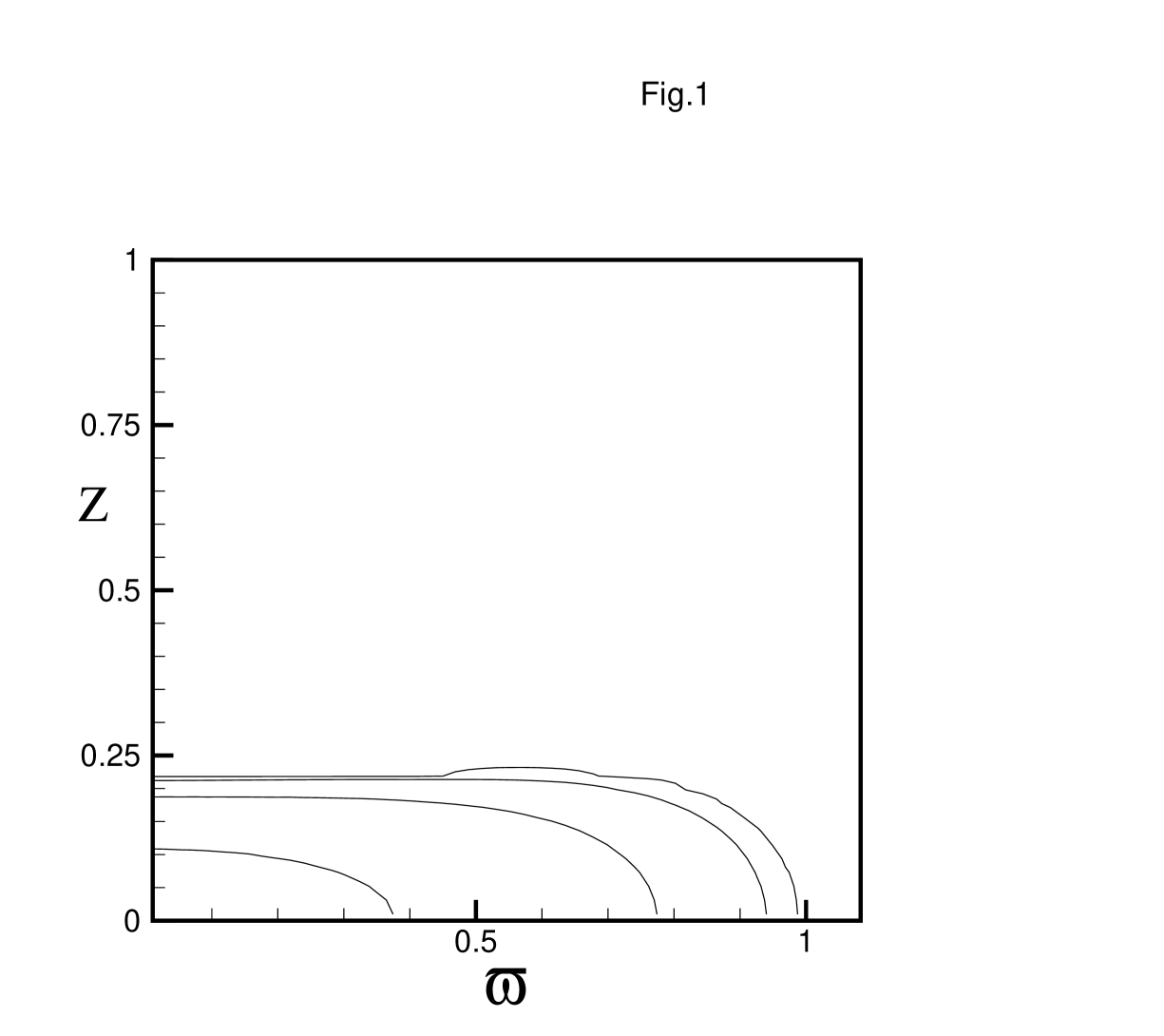
FIG. 1.: Density contours of the initial model with resolution $N_{\varpi}=N_{z}=128$ are shown in the $x-z$ plane. The maximum density is located at the center and is normalized to unity. The density contours are at levels of 0.5, 0.05, 0.005, and 0.0005.

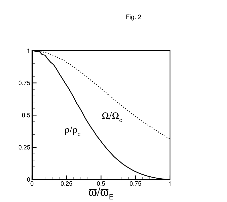
FIG. 2.: The normalized angular velocity $\Omega(\varpi)/\Omega_{\rm C}$ and equatorial plane density $\rho(z=0)/\rho_{\rm C}$ in the initial model given in Fig. 1 are shown. Here, $\Omega_{\rm C}$ and $\rho_{\rm C}$ are, respectively, the angular velocity and density at the center of the model.

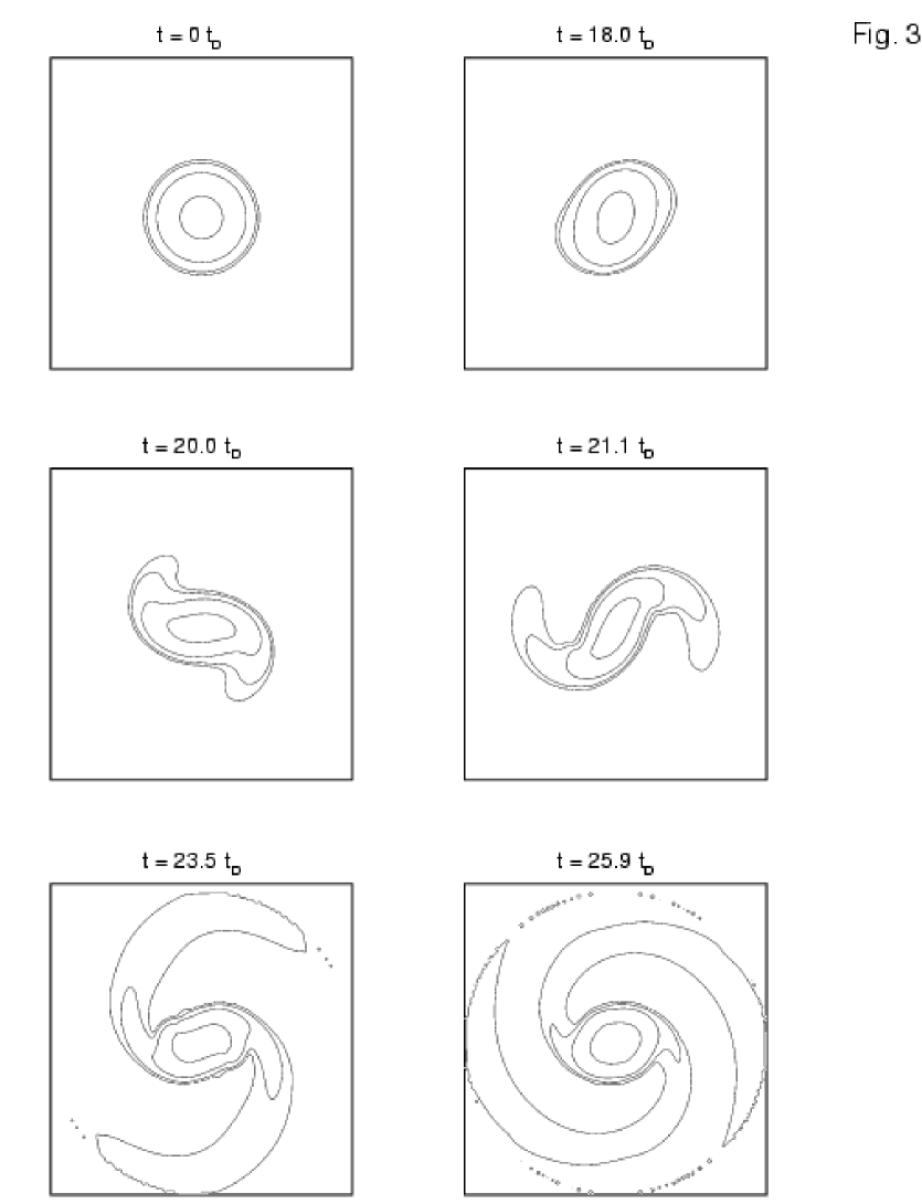
FIG. 3.: The development of the bar mode into the nonlinear regime is shown using 2-D density contours in the equatorial plane for model L3. The maximum (central) density has been normalized to unity at the initial time, and the contour levels are at 0.5, 0.05, 0.005, and 0.005. The model rotates in the counterclockwise direction.

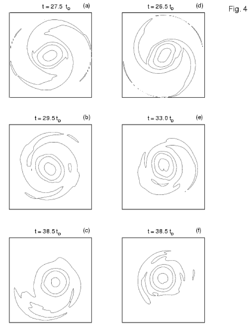
FIG. 4.: Density contours in the equatorial plane for the later stages of models D1 (a-c) and D2 (d-f) are shown. The contour levels are the same as in Fig. 3, and time is measured from the initial moments in the respective simulations.

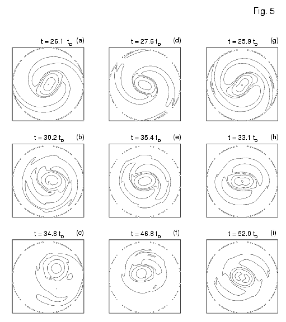
FIG. 5.: Same as Fig. 4 for models L1 (a-c), L3 (d-f), and L2 (g-i).

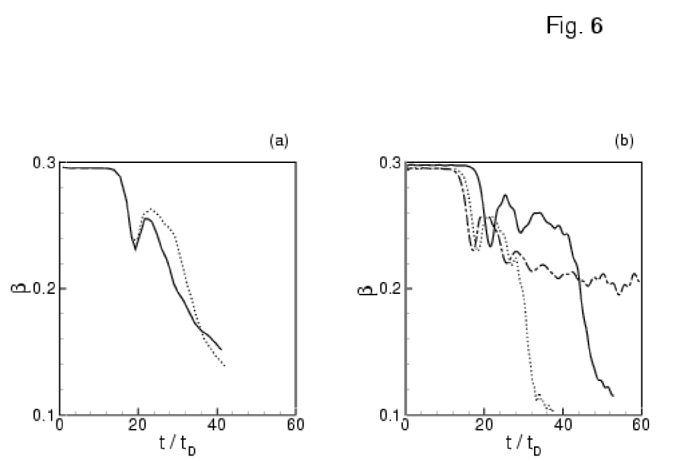
FIG. 6.: Plots of the stability parameter $\beta$ are shown for models D1 (dotted line) and D2 (solid line) in frame (a) and models L1 (dotted line), L3 (solid line) and L2 (dashed-dotted line) in frame (b).

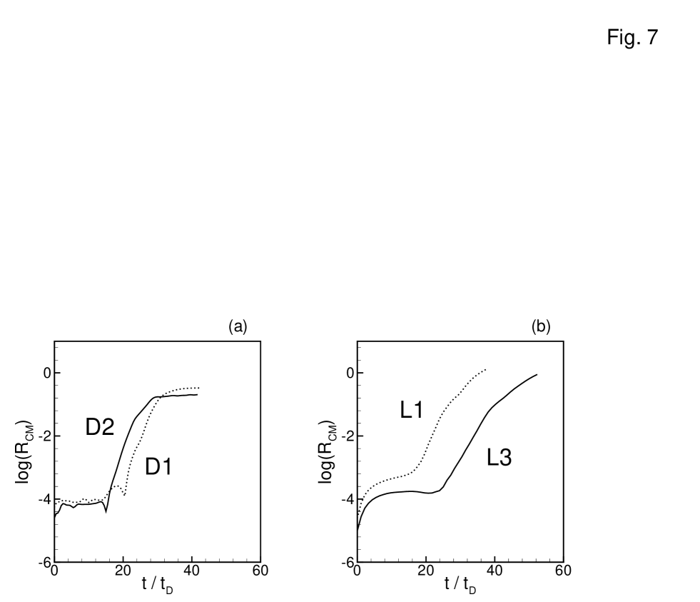
FIG. 7.: The position of the system center of mass is shown as a function of time. (a) Models D1 (dotted line) and D2 (solid line) (b) Models L1 (dotted line) and L3 (solid line). Note that the use of $\pi$-symmetry in model L2 prohibits the development of center of mass motion.

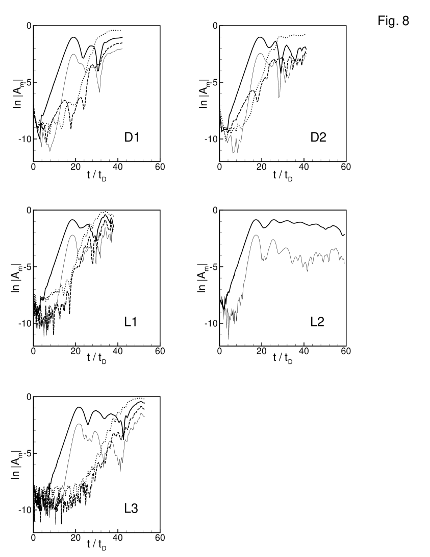
FIG. 8.: The growth of the amplitudes $|A_{m}|$ for $m=1$ (dotted line), $m=2$ (thick solid line), $m=3$ (dashed line), and $m=4$ (thin solid line) is shown. The amplitudes were calculated in the equatorial plane in a ring with radius $\varpi=0.354$ for runs D1, D2, L1, and L2, and radius $\varpi=0.344$ for run L3.

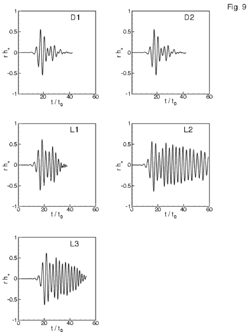
FIG. 9.: The gravitational waveform $h_{+}$ for an observer located on the axis at $\theta=0$, $\varphi=0$ of a spherical coordinate system centered on the source is shown as a function of time for all models. The quantity plotted is actually $r\,h_{+}$, where $r$ is the distance to the source. The quantities $h_{+}$ and $r$ have been normalized to $(GM/c^{2}R_{e})^{2}$ and $R_{e}$, respectively.

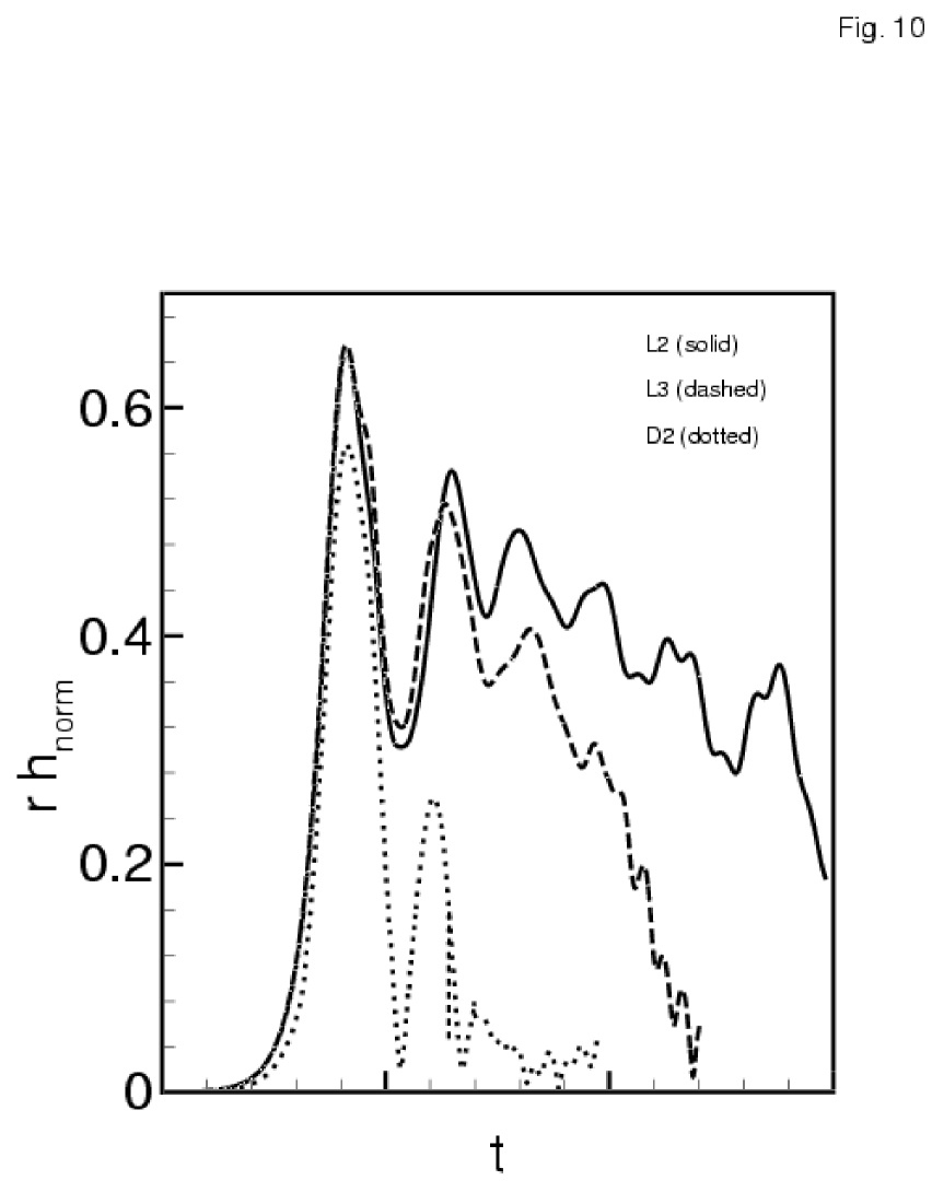
FIG. 10.: The quantity $r\,h_{\rm norm}=r\,(h_{+}^{2}+h_{\times}^{2})^{1/2}$ is shown as a function of time for all models. The normalization is the same as in Fig. 9. The absolute scale of the time axis is not labeled as the L3 and D2 curves have been horizontally shifted in order to align their intial peaks with that of the L2 curve.

Ref.	$N$	$\beta$	code	$\pi$-symm	$t_{{\rm bar}\;{\rm max}}$	$t_{\rm final}$	$\Delta t_{\rm bar}$	remarks
[30]	1.5	0.33	Eulerian	yes	2.5 $t_{\rm c}$	9.5 $t_{\rm c}$	$>7.0$ $t_{\rm c}$	central bar at $t_{\rm final}$
[30]	1.5	0.33	SPH	no	2.0 $t_{\rm c}$	9.5 $t_{\rm c}$	$>7.5$ $t_{\rm c}$	central bar at $t_{\rm final}$
[31]	1.8	0.31	Eulerian	yes	11.3 $t_{\rm c}$	19.4 $t_{\rm c}$	$>8.1$ $t_{\rm c}$	central bar at $t_{\rm final}$
[26]	1.5	0.30	Eulerian	no	10 $t_{\rm c}$	15.5 $t_{\rm c}$	$\sim 5.5$ $t_{\rm c}$	no bar at $t_{\rm final}$
[26]	1.5	0.30	SPH	no	8.2 $t_{\rm c}$	16 $t_{\rm c}$	$\sim 7.8$ $t_{\rm c}$	no bar at $t_{\rm final}$
[34]	1.5	0.30	SPH	no	5.7 $t_{\rm c}$	15.9 $t_{\rm c}$	$\sim 7.9$ $t_{\rm c}$	bar gone by $t\sim 13.6\;t_{\rm c}$
[27]	1.5	0.30	Eulerian	yes	6.8 $t_{\rm c}$	24.3 $t_{\rm c}$	$>17.5$ $t_{\rm c}$	central bar at $t_{\rm final}$
[21]	1.5	0.327	Eulerian	no	6.8 $t_{\rm c}$	12.3 $t_{\rm c}$	$>5.5$ $t_{\rm c}$	central bar at $t_{\rm final}$
[35]	1.5	0.304	Eulerian	no	10.1 $t_{\rm c}$	14.4 $t_{\rm c}$	$>4.3$ $t_{\rm c}$	central bar at $t_{\rm final}$
[35]	1.5	0.327	Eulerian	no	n/a	11.2 $t_{\rm c}$	n/a	central bar at $t_{\rm final}$

TABLE I.: Properties of long-duration simulations of the bar mode instability. $t_{{\rm bar}\;{\rm max}}$ is the time at which the bar reaches its maximum elongation and $t_{\rm final}$ is the end of the simulation. The length of time the bar persists is $\Delta t_{\rm bar}$. In this table, time is measured in units of $t_{\rm c}$, where $1\;t_{\rm c}$ = 1 central initial rotation period (cirp).

model	code	grid size	$\pi$-symmetry	$\rho_{\rm low}$	persistent	$|J_{{\rm bar}\;{\rm max}}-J_{o}|/J_{o}$
		$N_{\varpi}\times N_{z}\times N_{\varphi}$			bar
D1	${\cal D}$	$64\times 64\times 64$	no	$10^{-10}$	no	$2.6\times 10^{-2}$
D2	${\cal D}$	$64\times 64\times 128$	no	$10^{-10}$	no	$5.1\times 10^{-2}$
L1	${\cal L}$	$64\times 64\times 128$	no	$10^{-7}$	no	$5.0\times 10^{-3}$
L2	${\cal L}$	$64\times 64\times 64$	yes	$10^{-7}$	yes	$5.0\times 10^{-3}$
L3	${\cal L}$	$128\times 128\times 128$	no	$10^{-7}$	yes	$5.2\times 10^{-3}$

TABLE II.: Basic properties of the models run on the ${\cal D}$ and ${\cal L}$ codes are shown. Note that model L2 was actually run with $\pi$-symmetry, giving an effective resolution of 128 zones in the angular direction. $\rho_{\rm low}$ is the minimum density in the “vacuum” regions; see Sec. III B. The last column shows the loss of total angular momentum $J$ at the time that $\beta$ reaches its first local minimum and the bar reaches it maximum elongation for each model; cf. Fig. 6. $J_{o}$ is the initial total angular momentum in the model.

model	$d\ln|A_{2}|/dt$	$d\ln|A_{4}|/dt$	$\sigma_{2}$	$\sigma_{4}$	$W_{2}$	$W_{4}$
	[$t_{\rm D}^{-1}$]	[$t_{\rm D}^{-1}$]	[$t_{\rm D}^{-1}$]	[$t_{\rm D}^{-1}$]	[$t_{\rm D}^{-1}$]	[$t_{\rm D}^{-1}$]
D1	0.54	0.98	1.5	3.2	0.75	0.80
D2	0.55	1.1	1.5	3.0	0.75	0.75
L1	0.55	0.94	2.0	3.9	1.0	0.98
L2	0.55	1.0	2.0	4.0	1.0	1.0
L3	0.55	1.1	2.0	4.0	1.0	1.0

TABLE III.: The growth rates, eigenfrequencies, and pattern speeds for the $m=2$ and $m=4$ modes are given for all runs. Notice that the pattern speeds $W_{2}\sim W_{4}$ for all models, indicating that the $m=4$ mode is a harmonic of the bar mode.

REFERENCES

- [1] Currently at Los Alamos National Laboratory, Los Alamos, NM 87545
- [2] See, e.g., articles in Gravitational Wave Detection, eds. K. Tsubono, M.-K. Fugimoto, and K. Kuroda (Universal Academic Press, Tokyo, 1996) for recent articles describing these interferometers.
- [3] W. Johnson and S. Merkowitz, Phys. Rev. Lett. 70, 2367 (1993)
- [4] G. Harry, T. Stevenson, and H. Paik, Phys. Rev. D, 54, 2409 (1996).
- [5] K.S. Thorne, in Black Holes and Relativistic Stars, Proceedings of a Conference in Memory of S. Chandrasekhar, ed. R. M. Wald (University of Chicago Press, Chicago, 1998)
- [6] S. Shapiro and A. Lightman, Astrophys. J. 207, 263 (1976).
- [7] B. Schutz, in Dynamical Spacetimes and Numerical Relativity, edited by J. Centrella (Cambridge University Press, New York, 1986).
- [8] D. Lai and S. L. Shapiro, Astrophys. J. 442, 259 (1995).
- [9] K. Thorne, in Proceedings of IAU Symposium 165, Compact Stars in Binaries, edited by J. van Paradijs, E. van den Heuvel, and E. Kuulkers (Kluwer, Dordrecht, 1996).
- [10] K. Thorne, in Proceedings of the Snowmass 95 Summer Study on Particle and Nuclear Astrophyiscs and Cosmology, edited by E. W. Kolb and R. Peccei (World Scientific, Singapore, 1996).
- [11] A. Hayashi, Y. Eriguchi, and M. Hashimoto, Astrophys. J. 492, 286 (1998).
- [12] R. Wagoner, Astrophys. J. 278, 345 (1984).
- [13] B. Schutz, Class. Quantum Gravity 6, 1761 (1989).
- [14] F. Rasio and S. Shapiro, Astrophys. J. 401, 226 (1992); Astrophys. J. 432, 242 (1994).
- [15] X. Zhuge, J. Centrella, and S. McMillan, Phys. Rev. D, 50, 6247 (1994); Phys. Rev. D, 54, 7261 (1996).
- [16] J. Tassoul, Theory of Rotating Stars (Princeton University Press, Princeton, 1978).
- [17] S. Shapiro and S. Teukolsky, Black Holes, White Dwarfs, and Neutron Stars (Wiley, New York, 1983).
- [18] R. Durisen and J. Tohline, in Protostars and Planets II, edited by D. Black and M. Matthews (Univ. of Arizona Press, Tucson, 1985).
- [19] R. Managan, R. Astrophys. J. 294, 463 (1985).
- [20] J. Imamura, J. Friedman, and R. Durisen, Astrophys. J. 294, 474 (1985).
- [21] B. Pickett, R. Durisen, and G. Davis, Astrophys. J. 458, 714 (1996).
- [22] J. Toman, J. N. Imamura, B. K. Pickett, and R. H. Durisen, Astrophys. J. 497, 370 (1998).
-
[23]
N. Stergioulas, 1998, in Living Reviews in Relativity,
http://www.livingreviews.org/Articles/Volume1/1998-8stergio/. - [24] J. Tohline, R. Durisen, and M. McCollough, Astrophys. J. 298, 220 (1985) [TDM].
- [25] J. Houser, J. Centrella, and S. Smith, Phys. Rev. Lett. 72, 1314 (1994).
- [26] S. Smith, J. Houser, and J. Centrella, Astrophys. J. 458, 236 (1996).
- [27] K. C. B. New, Ph.D. Thesis, Louisiana State University (1996).
- [28] J. Woodward, Ph.D. Thesis, Louisiana State University (1992).
- [29] H. Williams and J. Tohline, Astrophys. J. 315, 594 (1987).
- [30] R. Durisen, R. Gingold, J. Tohline, and A. Boss, Astrophys. J. 305, 281 (1986).
- [31] H. Williams and J. Tohline, Astrophys. J. 334, 449 (1988).
- [32] L. Hernquist and N. Katz, Astrophys. J. Suppl. 70, 419 (1989).
- [33] S. Smith, J. Centrella, and S. Clancy, Astrophys. J. Suppl. 94, 789 (1994).
- [34] J. Houser and J. Centrella, Phys. Rev. D, 54, 7278 (1996).
- [35] J. N. Imamura, R. H. Durisen, and B. K. Pickett, Astrophys. J., in press (1999).
- [36] I. Hachisu, Astrophys. J. Suppl. 61, 479 (1986).
- [37] P. Bodenheimer and J. Ostriker, Astrophys. J. 180, 159 (1973).
- [38] J. Tohline, Ph.D. Thesis, University of California at Santa Cruz (1978).
- [39] K. C. B. New and J. E. Tohline, Astrophys. J. 490, 311 (1997).
- [40] R. Bowers and J. Wilson, Numerical Modeling in Applied Physics and Astrophysics (Boston, Jones and Bartlett, 1991).
- [41] D. L. Powers, Boundary Value Problems, 3rd Edition, (Harcourt, Brace, and Jovanovich, Florida, 1987).
- [42] D. Lynden-Bell and J. P. Ostriker, Mon. Not. R. Astron. Soc. 136, 293 (1967).
- [43] S. Chandrasekhar, Ellipsoidal Figures of Equilibrium (New Haven, Yale University Press, 1969).
- [44] C. Misner, K. Thorne, and J. Wheeler Gravitation (Freeman, New York, 1973).
- [45] C. Kochanek, S. Shapiro, S. Teukolsky, and D. Chernoff, Astrophys. J. 358, 81 (1990).
- [46] L. S. Finn and C. Evans, Astrophys. J. 351, 588 (1990).
- [47] J. E. Cazes and J. E. Tohline, Astrophys. J., in press (April 2000).
- [48] L. Bildsten and C. Cutler, Astrophys. J. 400, 175 (1992).
- [49] C. S. Kochanek, Astrophys. J. 398, 234 (1992).
- [50] S. P. Clancy, Ph.D. Thesis, University of Texas at Austin (1989).
- [51] S. C. Smith, Ph.D. Thesis, Drexel University (1993).
- [52] D. Mihalas and B. Mihalas, Foundations of Radiation Hydrodynamics (Oxford University Press, 1984).
- [53] J. Wilson, in Sources of Gravitational Radiation, ed. L. Smarr (Cambridge University Press, 1979).
- [54] J. Hawley, L. Smarr, and J. Wilson, Astrophys. J. Suppl. 55, 211 (1984).
- [55] M. Norman, J. Wilson, and R. Barton, Astrophys. J. 239, 968 (1980).
- [56] J. M. Stone and M. L. Norman, Astrophys. J., Suppl. Ser. 80, 753 (1992).
- [57] W. Press, B. Flannery, S. Teukolsky, and W. Vetterling, Numerical Recipies, 2d. ed. (Cambridge University Press, 1992).
- [58] J. Meijerink and H. van der Vorst, J. Computat. Phys. 44, 134 (1981).
- [59] J. Tohline, Astrophys. J. 253, 866.
- [60] J. Woodward, J. Tohline, and I. Hachisu, Astrophys. J. 420, 247 (1994).
- [61] B. van Leer, J. Computat. Phys. 23, 276 (1976).
- [62] G. van Albada, B. van Leer, and W. Roberts, Jr. Astron. Astrophys. 108, 76 (1982).
- [63] G. van Albada, Astron. Astrophys. 142, 491 (1985).
- [64] H. S. Cohl, X.-H. Sun, and J. E. Tohline, in Proc. 8th SIAM Conference on Parallel Processing for Scientifc Computing, eds. M. Heath et al. (SIAM, Philadelphia, 1997) .