Total intensity and polarized emission of the parsec-scale jet in 3C 345

Abstract

We have studied the parsec-scale structure of the quasar 3C 345 at $\lambda\lambda$ 1.3, 2, 3.6, and 6 cm, using total intensity and linear polarization images from 3 epochs of VLBA observations made in 1995.84, 1996.41, and 1996.81. The images show an unresolved “core” and a radio jet extending over distances up to 25 milliarcseconds. At 1.3 and 2 cm, images of the linearly polarized emission reveal an alignment of the electric vector with the extremely curved inner section of the jet. At 6 cm, the jet shows strong fractional polarization ($m$$\sim$15%), with the electric vector being oriented perpendicular to the jet. This is consistent with the existence of a transition from the shock-dominated to the plasma interaction-dominated emission regimes in the jet, occurring at a distance of $\sim$1.5 milliarcseconds from the “core”.

1 Introduction

The QSO 3C 345 (V$\sim$16; $z$=0.5928, Marziani et al. mar96 (1996)) presents one of the best examples of apparent superluminal motion in a core-dominated extragalactic radio source, with components traveling in the parsec-scale jet along curved trajectories at apparent speeds of up to 10$c$ (Zensus et al. 1995a ).

3C 345 has been monitored using the Very Long Baseline Interferometry (VLBI) technique since 1979 (Unwin et al. unw83 (1983), Biretta et al. bir86 (1986), Brown et al. bro94 (1994), Wardle et al. war94 (1994), Rantakyrö et al. ran95 (1995), Zensus et al. 1995a , 1995b , Lobanov lob96 (1996), Taylor tay98 (1998), Lobanov & Zensus lob99 (1999)). On arcsecond scales the source contains a compact region at the base of a 4^′′ jet that is embedded in a diffuse steep-spectrum halo (Kollgaard et al. kol89 (1989)).

From astrometric measurements, the parsec-scale core has been shown to be stationary within uncertainties of 20 $\mu$as/yr (Bartel et al. bar86 (1986)). The parsec-scale jet consists of several prominent enhanced emission regions (jet components) apparently ejected at different position angles (P.A. ranging from 240^∘ to 290^∘) with respect to the jet core. The components move along curved trajectories that can be approximated by a simple helical geometry (Steffen et al. ste95 (1995), Qian et al. qia96 (1996)). The curvature of the trajectories may be caused by some periodic process at the jet origin, e.g. orbital motion in a binary black hole system (Lobanov lob96 (1996)) or Kelvin-Helmholtz instabilities. At lower frequencies, the jet extends to the NW direction, turning northwards at $\geq$20 milliarcseconds (mas) distance from the core.

VLBI polarimetry of nonthermal radio sources can provide stringent information about the physical conditions in the parsec-scale jets. Since the early works of Cotton et al. (cot84 (1984)), substantial progress has been achieved in this area, particularly benefiting from the enhanced observing capabilities of the VLBA. The VLBA antennas have standardized feeds with low instrumental polarization, and use high-performance receivers. A new method of self-calibration of the polarimetric VLBI observations (Leppänen et al. lep95 (1995)) has made it feasible to measure the fractional polarization with an accuracy of 0.15%, by using the target source itself as a calibrator. The technique is non-iterative and insensitive to the structure of the polarization calibrator.

In 1979–1993, 3C 345 was monitored using VLBI at several frequencies. These observations have allowed the determination of the trajectories and kinematic properties of the jet components (cf. Zensus et al. 1995a ). In this paper we extend this effort, and present three epochs of multi-frequency VLBA observations which also include polarization information. The observations were made in 1995.84, 1996.41, and 1996.81 at observing frequencies of 22, 15, 8.4, and 5 GHz. We describe the observations and data reduction in Sect. 2. In Sect. 3, we present the total intensity, polarization, and spectral index images of the parsec-scale jet in 3C 345, and discuss the properties of the jet emission.

Throughout this paper, we use a Hubble constant $H_{0}$=100$h$ km s^-1 Mpc^-1 and the deceleration parameter $q_{0}$=0.5. For 3C 345, this results in a linear scale of 3.79 $h^{-1}$ pc mas^-1. A proper motion of 1 mas yr^-1, then, translates into an apparent speed of $\beta_{\rm app}$=19.7 $h^{-1}$$c$. We use the positive definition of spectral index, $\alpha$ ($S\propto\nu^{+\alpha}$).

2 VLBA observations

We carried out multi-frequency observations of 3C 345 at three epochs, 1995.84, 1996.41, and 1996.81, using all 10 VLBA antennas. The observations are summarized in Table 1. 3C 345 was observed at each frequency with a 5 min scan every 20 min for a total period of almost 14 h. The bandwidth achieved in all cases was 16 MHz. The data were registered in VLBA format, with an aggregate data rate of 64 Mbits/s, recording 4 channels with 1-bit sampling (mode 64-4-1, see Romney rom85 (1985)). Some calibrator scans (the calibrator sources are listed in Table 1) were inserted during the observations.

Table 1: 3C 345 observation and map parameters

			3C 345 image parameters
	Freq.				Beam
Epoch	$\nu$	Calibrators	Beam size		P.A.	$S_{\rm tot}$a		$S_{\rm peak}$b		Contours in Fig. 1
	[GHz]		[mas]			[Jy]		[Jy/beam]		[(mJy/beam)$\times$(levels)]
1995.84	22	3C 279	0.480$\times$	0.326	–15$\hbox to0.0pt{.\hss}^{\circ}$0	6.98$\pm$	0.14	2.56$\pm$	0.05	5.1$\times$(	–1,1,1.4,$\cdots$,256,362)
	15	3C 279	0.690$\times$	0.453	–0$\hbox to0.0pt{.\hss}^{\circ}$7	7.98$\pm$	0.16	3.66$\pm$	0.07	7.2$\times$(	–1,1,1.4,$\cdots$,256,362)
	8.4	3C 84	1.254$\times$	0.731	2$\hbox to0.0pt{.\hss}^{\circ}$9	9.32$\pm$	0.18	4.46$\pm$	0.09	6.7$\times$(	–1,1,1.4,$\cdots$,362,512)
	5	3C 84	2.443$\times$	1.348	–21$\hbox to0.0pt{.\hss}^{\circ}$0	7.51$\pm$	0.15	4.41$\pm$	0.09	4.4$\times$(	–1,1,1.4,$\cdots$,512,724.1)
1996.41	22	NRAO 91	0.433$\times$	0.316	–3$\hbox to0.0pt{.\hss}^{\circ}$1	4.51$\pm$	0.09	1.80$\pm$	0.04	3.7$\times$(	–1,1,1.4,$\cdots$,256,362)
	15	NRAO 91	0.624$\times$	0.457	–7$\hbox to0.0pt{.\hss}^{\circ}$3	6.70$\pm$	0.13	2.67$\pm$	0.05	5.3$\times$(	–1,1,1.4,$\cdots$,256,362)
	8.4	OQ 208	1.136$\times$	0.810	–7$\hbox to0.0pt{.\hss}^{\circ}$9	7.49$\pm$	0.15	3.55$\pm$	0.07	5.3$\times$(	–1,1,1.4,$\cdots$,362,512)
	5	OQ 208	1.967$\times$	1.318	–9$\hbox to0.0pt{.\hss}^{\circ}$5	7.21$\pm$	0.14	3.91$\pm$	0.08	3.9$\times$(	–1,1,1.4,$\cdots$,512,724.1)
1996.81	22	–	0.451$\times$	0.322	–15$\hbox to0.0pt{.\hss}^{\circ}$5	4.61$\pm$	0.09	2.09$\pm$	0.04	4.2$\times$(	–1,1,1.4,$\cdots$,256,362)
	15	3C 286	0.614$\times$	0.474	–6$\hbox to0.0pt{.\hss}^{\circ}$1	5.98$\pm$	0.12	2.72$\pm$	0.05	5.4$\times$(	–1,1,1.4,$\cdots$,256,362)
	8.4	3C 286	1.132$\times$	0.887	–16$\hbox to0.0pt{.\hss}^{\circ}$8	7.52$\pm$	0.15	3.59$\pm$	0.07	5.4$\times$(	–1,1,1.4,$\cdots$,362,512)
	5	3C 286	1.861$\times$	1.532	–15$\hbox to0.0pt{.\hss}^{\circ}$3	7.26$\pm$	0.15	4.29$\pm$	0.09	4.3$\times$(	–1,1,1.4,$\cdots$,512,724.1)

• Total flux density recovered in the map model. The calibration errors are always smaller than a 2%, which translates into the tabulated values for the uncertainties in $S_{\rm tot}$ and $S_{\rm peak}$.

• Peak of brightness in the map.

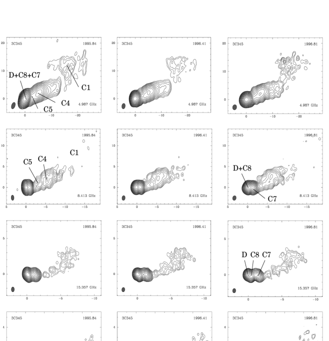
Figure 1: VLBA total intensity flux images of 3C 345 for the three epochs and the four frequencies. The map parameters are given on Table 1. The synthesized interferometric beams are represented at the bottom left of each image. Notice that the scales are not the same at different frequencies.

The data were correlated at the NRAO VLBA Array Operations Center in Socorro, NM, US. A 2-s correlator pre-averaging time was used. Interferometer fringes were detected on all baselines for the target source and the calibrators. The data were processed using aips. The visibility amplitudes were calibrated using antenna gains and system temperatures measured at each antenna. The fringe fitting of the residual delays and fringe rates was performed independently for both parallel hands of the correlated data, and the solutions obtained were then referenced to a common reference antenna (Los Alamos for all cases). After the fringe fitting, the data were averaged in frequency and exported into difmap (Shepherd et al. she94 (1994)) for self-calibration and imaging. The data were further time-averaged, with the averaging times selected individually at each frequency so as not to exceed the respective coherence times. We applied the clean algorithm and self-calibration in several cycles to produce the total intensity images.

2.1 Data analysis of the total intensity data

In order to quantify the source structure, we fitted models consisting of elliptical Gaussian components to each of the self-calibrated data sets, using the tasks modelfit and modfit of the Caltech Package (Pearson & Readhead pea88 (1988)). For the purpose of studying the spectral properties of the jet, we reproduced all images in a consistent fashion, by selecting matching $uv$-ranges at all frequencies and by restoring the final images with the same circular beam.

2.2 Imaging the polarized emission

Images of the linearly polarized intensity were obtained. The instrumental polarization was determined using the feed solution algorithm developed by Leppänen et al. (lep95 (1995)). The average accuracy of the antenna D-terms was better than 1%. For some antennas, larger values of the D-terms were found at higher frequencies: Brewster—4% at 22 GHz; OVRO—6–8% at 22 GHz and up to 4% at 15 GHz; Saint Croix—5% in 1996.81 at 22 GHz.

We transferred the clean component models from the total intensity ($I$) images back into aips and then used the task imagr to produce the Stokes $U$ and $Q$ images of 3C 345. The distribution of the polarized flux $p$ and the position angle of the polarized emission was obtained from the combination of the $U$ and $Q$ images. The registration of the $I$ and $P$ maps to within a small fraction of a fringe spacing was assured by using the same set of antenna phases in the $U$ and $Q$ imaging.

The final step in the polarization calibration was to determine the absolute offset between the right and left hand phases at the reference station. This can be done in one of three possible ways: a) by observing a radio source with a known electric vector position angle $\chi$, b) by comparing the VLBI maps with VLA maps (that should account for the total polarized intensity), and/or c) by comparing the values of leakage of RCP into the left feed and LCP into the right feed in the receivers (quantified as “D-terms”) of the antennas with values from neighbor epochs (relying in their time stability). We have applied the approaches b) & c) in our data reduction. For the epochs and frequencies without such information, the right- and left- hand offsets were introduced ad hoc, based on the consistency with the calibration at other frequencies and epochs (for instance, we were assuming that the outer, extended components cannot change their $\chi$ very rapidly from one epoch to another). We summarize the polarization calibration for all epochs and frequencies in Table 2.

Table 2: Polarization calibration summary

	22 GHz	15 GHz	8.4 GHz	5 GHz
1995.84	D-terma/VLAb	D-term.a/VLAb	VLAb	VLAb
1996.41	VLAb	Man.c	VLAb	Man.c
1996.81	D-termd	D-termd	Man.c	Man.c

• Calibrated comparing with the D-terms at epoch 1995.83 (Alberdi, priv. comm.).

• Calibrated using VLA images.

• The right/left hand offsets were introduced manually, based on the consistency with the calibration at other frequencies and epochs.

• Calibrated comparing with the D-Terms at epoch 1996.85 (Gómez, priv. comm.).

At frequencies $\geq$5 GHz, the ionospheric effects are negligible and can be safely ignored. We also do not apply Faraday rotation corrections to the observed electric vector position angles, relying on the results of Taylor (tay98 (1998)), who reports small rotation measurements ($RM=-130$ rad m^-2 at the core and –70 rad m^-2 at the parsec-scale jet, derived from a least-squares fit to the polarization angle measurements between 8.1 and 15.2 GHz) at frequencies higher than 5 GHz.

3 Results and discussion

3.1 Total intensity images and model fits

The total intensity images of 3C 345 are shown in Fig. 1. The parameters of the images are given in Table 1. The quality of the data and the performance of the VLBA antennas and correlator were excellent. The model fits for all images are presented in Table 3.

The errors in component position determined at each epoch are typically smaller than a tenth of a beamwidth, but to be conservative we have assumed a magnitude of a fifth of beamwidth. That means, approximatively, 0.08 mas for the 22 GHz results, 0.11 mas for 15 GHz, 0.19 mas for 8.4 GHz, and 0.32 mas for 5 GHz. The errors for the other parameters were determined combining the statistical standard errors provided by the task erfit (revised and improved version of errfit) from the Caltech Package, and some statistical and empirical considerations.

3.1.1 The models at 22 GHz

Table 3: Model fitting results

		$S^{\rm a}$		$r^{\rm b}$		$\theta^{\rm c}$		$a^{\rm d}$		$b/a^{\rm e}$		$\phi^{\rm f}$
		[Jy]		[mas]		[∘]		[mas]				[∘]
		——————— 22 GHz ———————
1995.84	Core (D)	2.730$\pm$	0.140	—		—		0.13$\pm$	0.01	1.0		—
	C8	2.252$\pm$	0.110	0.40$\pm$	0.08	-122$\pm$	11	0.25$\pm$	0.01	0.66$\pm$	0.01	47$\pm$	1
	C7	1.214$\pm$	0.060	1.20$\pm$	0.08	-95$\pm$	4	0.51$\pm$	0.01	0.55$\pm$	0.01	71$\pm$	1
	Jet	0.400$\pm$	0.020	6.20$\pm$	0.14	-68$\pm$	1	4.03$\pm$	0.14	0.61$\pm$	0.03	58$\pm$	3
1996.41	Core (D)	2.168$\pm$	0.110	—		—		0.16$\pm$	0.01	1.0		—
	C8	1.184$\pm$	0.060	0.48$\pm$	0.08	-118$\pm$	9	0.30$\pm$	0.01	0.60$\pm$	0.01	-23$\pm$	1
	C7	0.884$\pm$	0.050	1.36$\pm$	0.08	-93$\pm$	3	0.53$\pm$	0.01	0.60$\pm$	0.01	66$\pm$	1
	Jet	0.334$\pm$	0.017	5.21$\pm$	0.11	-73$\pm$	2	6.8$\pm$	0.2	0.33$\pm$	0.02	-64$\pm$	1
1996.81	Core (D)	1.618$\pm$	0.200	—		—		0.14$\pm$	0.01	1.00		—
	C9	1.082$\pm$	0.200	0.16$\pm$	0.08	-100$\pm$	26	0.07$\pm$	0.01	0.5$\pm$	0.1	119$\pm$	8
	C8	1.087$\pm$	0.050	0.67$\pm$	0.08	-108$\pm$	7	0.39$\pm$	0.01	0.67$\pm$	0.01	122$\pm$	1
	C7	0.694$\pm$	0.040	1.55$\pm$	0.08	-93$\pm$	3	0.70$\pm$	0.01	0.52$\pm$	0.01	59$\pm$	1
	Jet	0.230$\pm$	0.012	5.9$\pm$	0.1	-72$\pm$	4	5.0$\pm$	0.2	0.5$\pm$	0.2	-51$\pm$	2
		——————— 15 GHz ———————
1995.84	Core (D)	2.616$\pm$	0.200	—		—		0.15$\pm$	0.01	1.0		—
	C8	3.135$\pm$	0.200	0.38$\pm$	0.11	-120$\pm$	16	0.28$\pm$	0.01	0.45$\pm$	0.08	-129$\pm$	1
	C7	1.779$\pm$	0.090	1.19$\pm$	0.11	-95$\pm$	5	0.59$\pm$	0.02	0.46$\pm$	0.01	74$\pm$	1
	Jet	0.556$\pm$	0.028	5.8$\pm$	0.3	-74$\pm$	2	6.2$\pm$	0.1	0.30$\pm$	0.01	-56$\pm$	1
1996.41	Core (D)	2.501$\pm$	0.130	—		—		0.12$\pm$	0.01	1.0		—
	C8	2.227$\pm$	0.110	0.46$\pm$	0.11	-115$\pm$	13	0.32$\pm$	0.01	0.85$\pm$	0.01	7$\pm$	1
	C7	1.544$\pm$	0.080	1.36$\pm$	0.11	-93$\pm$	5	0.60$\pm$	0.01	0.58$\pm$	0.01	66$\pm$	1
	Jet	0.440$\pm$	0.022	6.0$\pm$	0.3	-72$\pm$	2	4.0$\pm$	1.0	0.5$\pm$	0.2	128$\pm$	1
1996.81	Core (D+C9)	2.844$\pm$	0.140	—		—		0.16$\pm$	0.01	1.0		—
	C8	1.762$\pm$	0.090	0.57$\pm$	0.11	-108$\pm$	11	0.38$\pm$	0.01	0.79$\pm$	0.01	97$\pm$	1
	C7	1.017$\pm$	0.050	1.48$\pm$	0.11	-93$\pm$	4	0.70$\pm$	0.01	0.50$\pm$	0.01	59$\pm$	1
	Jet	0.374$\pm$	0.020	5.89$\pm$	0.6	-73$\pm$	3	4.9$\pm$	0.1	0.39$\pm$	0.01	-55$\pm$	1
		——————— 8.4 GHz ———————
1995.84	Core (D)	2.746$\pm$	0.197	—		—		0.22$\pm$	0.10	1.0		—
	C8	2.337$\pm$	0.185	0.33$\pm$	0.19	-119$\pm$	30	0.21$\pm$	0.02	0.72$\pm$	0.08	106$\pm$	22
	C7	2.490$\pm$	0.195	1.09$\pm$	0.19	-93$\pm$	9	0.59$\pm$	0.01	0.57$\pm$	0.01	66$\pm$	1
	C5b	0.082$\pm$	0.020	2.35$\pm$	0.3	-92$\pm$	10	1.0$\pm$	0.2	0.5$\pm$	0.2	100$\pm$	9
	C5a	0.141$\pm$	0.010	3.76$\pm$	0.19	-79$\pm$	3	1.16$\pm$	0.07	0.77$\pm$	0.07	105$\pm$	11
	C4	0.552$\pm$	0.028	6.29$\pm$	0.3	-69$\pm$	7	3.0$\pm$	0.2	0.7$\pm$	0.1	132$\pm$	2
	C1	0.203$\pm$	0.010	11.0$\pm$	0.3	-72$\pm$	9	8.4$\pm$	1.0	0.5$\pm$	0.4	112$\pm$	4
1996.41	Core (D)	2.097$\pm$	0.205	—		—		0.24$\pm$	0.01	1.0		—
	C8	2.304$\pm$	0.115	0.43$\pm$	0.19	-115$\pm$	24	0.32$\pm$	0.01	0.59$\pm$	0.06	-27$\pm$	2
	C7	2.081$\pm$	0.105	1.28$\pm$	0.19	-93$\pm$	8	0.63$\pm$	0.01	0.57$\pm$	0.01	67$\pm$	1
	C5	0.124$\pm$	0.010	2.26$\pm$	0.19	-93$\pm$	5	1.5$\pm$	0.5	0.5$\pm$	0.3	117$\pm$	2
	C4	0.713$\pm$	0.036	6.07$\pm$	1.0	-71$\pm$	8	4.36$\pm$	0.03	0.50$\pm$	0.01	126$\pm$	1
	C1	0.108$\pm$	0.010	11.8$\pm$	0.19	-73$\pm$	6	6.3$\pm$	0.2	0.41$\pm$	0.03	141$\pm$	2
1996.81	Core (D)	2.154$\pm$	0.110	—		—		0.15$\pm$	0.01	1.0		—
	C8	2.870$\pm$	0.130	0.54$\pm$	0.19	-107$\pm$	20	0.4$\pm$	0.2	0.84$\pm$	0.01	127$\pm$	20
	C7	0.893$\pm$	0.050	1.31$\pm$	0.19	-90$\pm$	9	0.51$\pm$	0.01	0.60$\pm$	0.02	63$\pm$	2
	C5b	0.767$\pm$	0.038	1.66$\pm$	0.19	-97$\pm$	7	0.7$\pm$	0.2	0.76$\pm$	0.01	49$\pm$	4
	C5a	0.171$\pm$	0.015	3.75$\pm$	0.19	-84$\pm$	8	2.45$\pm$	0.04	0.5$\pm$	0.1	106$\pm$	1
	C4	0.556$\pm$	0.030	6.60$\pm$	0.19	-69$\pm$	6	3.4$\pm$	0.5	0.66$\pm$	0.01	119$\pm$	1
	C1	0.131$\pm$	0.010	12.17$\pm$	1.0	-72$\pm$	7	7.0$\pm$	2.0	0.6$\pm$	0.2	141$\pm$	5
		——————— 5 GHz ———————
1995.84	Core (D)	1.892$\pm$	0.345	—		—		0.15$\pm$	0.10	1.0		—
	C8	1.695$\pm$	0.328	0.37$\pm$	0.32	-112$\pm$	41	0.49$\pm$	0.01	0.4$\pm$	0.2	87$\pm$	3
	C7	2.394$\pm$	0.130	1.08$\pm$	0.32	-90$\pm$	17	0.63$\pm$	0.01	0.4$\pm$	0.2	64$\pm$	1
	C5	0.189$\pm$	0.010	3.20$\pm$	0.32	-82$\pm$	6	2.2$\pm$	0.1	0.4$\pm$	0.2	97$\pm$	4
	C4	0.800$\pm$	0.040	6.30$\pm$	0.32	-69$\pm$	3	3.58$\pm$	0.03	0.54$\pm$	0.01	120$\pm$	1
	C1	0.305$\pm$	0.020	17.6$\pm$	0.5	-59$\pm$	2	17.2$\pm$	0.6	0.26$\pm$	0.02	152$\pm$	2
1996.41	Core (D)	1.100$\pm$	0.153	—		—		0.15$\pm$	0.10	1.0		—
	C8	2.279$\pm$	0.150	0.39$\pm$	0.32	-115$\pm$	40	0.3$\pm$	0.1	0.5$\pm$	0.1	-68$\pm$	19
	C7	2.343$\pm$	0.150	1.26$\pm$	0.32	-93$\pm$	14	0.69$\pm$	0.05	0.43$\pm$	0.03	68$\pm$	3
	C5	0.420$\pm$	0.030	3.76$\pm$	0.32	-85$\pm$	5	3.8$\pm$	0.2	0.37$\pm$	0.01	108$\pm$	1
	C4	0.700$\pm$	0.040	6.65$\pm$	0.32	-68$\pm$	3	3.50$\pm$	0.03	0.60$\pm$	0.01	104$\pm$	1
	C1	0.356$\pm$	0.010	17.3$\pm$	0.4	-61$\pm$	2	15.0$\pm$	1.0	0.49$\pm$	0.02	142$\pm$	2
1996.81	Core (D)	0.948$\pm$	0.100	—		—		0.15$\pm$	0.03	1.0		—
	C8	2.929$\pm$	0.150	0.49$\pm$	0.32	-112$\pm$	33	0.49$\pm$	0.01	0.66$\pm$	0.01	93$\pm$	1
	C7	2.025$\pm$	0.100	1.42$\pm$	0.32	-94$\pm$	13	0.84$\pm$	0.01	0.47$\pm$	0.01	64$\pm$	1
	C5	0.347$\pm$	0.020	4.03$\pm$	0.32	-82$\pm$	5	3.44$\pm$	0.02	0.4$\pm$	0.2	104$\pm$	1
	C4	0.677$\pm$	0.040	6.79$\pm$	0.32	-68$\pm$	3	3.57$\pm$	0.02	0.49$\pm$	0.01	104$\pm$	1
	C1	0.368$\pm$	0.020	16.7$\pm$	0.5	-62$\pm$	2	17.7$\pm$	0.3	0.36$\pm$	0.01	141$\pm$	1

• $S$, flux density of the Gaussian component. ^b $r$, distance to the main component. ^c $\theta$, position angle (defined north to west) of the component. ^d $a$, major axis at the FWHM of the elliptical Gaussian. ^e $b$, minor axis; $b/a$ ratio. ^f $\phi$, position angle of the major axis.

Table 3 lists the Gaussian fits for the data at 22 GHz. We can model the radio source reliably with four components, that we associate with the core D, the components C8 and C7, and a more extended emission to the NW labeled as “jet” (which contains the components identified with C5 and C4 at lower frequencies). Components C8 and C7 move away from the core, at angular speeds of 0.27$\pm$0.12 mas/yr (estimated from our three observations, and corresponding to an apparent speed of 5.3$\pm$2.3 $h^{-1}\,c$, uncertainties shown here and in the next subsections are statistical standard errors from a weighted linear fit to the core distances) and 0.35$\pm$0.12 mas/yr (7.0$\pm$2.3 $h^{-1}\,c$), respectively. In Fig. 2, we represent their proper motions by the changes of $r$ (distance to component D) with time. The inner components of the jet of 3C 345 have displayed complex trajectories in previous epochs. We cannot associate C8 with previous components, since it is new, component C7 has been observed before and displays acceleration from 1991 to our observing epochs. With our time span of a year we linearize the behavior of the C7 and C8 components to compute their apparent velocities. The comparison of the positions reported here with later observing epochs at the same frequencies should constrain the parameters of their kinematics.

Figure 2: Core separations for the jet components C7, C8, and C9 obtained from the model fits to the data at 15 and 22 GHz.

A better fit is obtained at the epoch 1996.81, by introducing a new component between the core D and C8, labeled as C9, very close to D, at 0.16 mas (P.A. $\sim-100^{\circ}$). The model fitted fluxes at D and C9 are strongly correlated. Different values for the flux densities of D and C9 (preserving constant the sum of both) provide almost the same values for the agreement factor in the fit. To the first order of accuracy, the fluxes at the core and C9 are close to $S_{\rm D}\sim 1.6$ Jy and $S_{\rm C9}\sim 1.0$ Jy.

We show the flux density evolution of the different components in Fig. 3, comparing also the values with the total flux density from the maps (Table 1) and the single dish measurements obtained in Metsähovi (Teräsranta et al. ter98 (1998), and priv. comm.). Lobanov & Zensus (lob99 (1999)) have applied a flare model to the observed variations of the 22 GHz flux density of the core during our observations. In their description, the core is at the late stages of the decay after a flare in 1995.2. The new component C9 may therefore be related to the flare in 1995.2. Similarly, previous components have been associated to flares. The periods of emergence of components are related to the periods of variability (see, e.g., Zhang et al. zha98 (1998)). This behavior is extremely clear for 3C 273 (Türler et al. tue99 (1999)). Following the work of Villata & Raiteri (vil99 (1999)) on Mkn 501, the most enhanced emission regions in the jets (called “components”) would be the result of the boosting of helical features caused by the viewing angle. The helicity would be generated by the rotation of a binary black hole system. A similar model was discussed for QSO 1928+738 by Hummel et al. (hum92 (1992)). The periodicity in the helix would then be correlated with the light-curve periodicity in the optical and radio, in this scenario.

Figure 3: Evolution of the flux densities at 22 (Teräsranta et al. ter98 (1998)) and 15 GHz (Univ. of Michigan) for the single dish flux, the total VLBI flux (from Table 1), and the fluxes of the model fit components (from Table 3).

The labeling of components follows Lobanov (lob96 (1996)). To identify our components with the trajectories reported before, we have combined our component positions with previous ones. We show in Fig. 4 our data combined with those mentioned above. There we can track C7, see how C6 is not detected now, and also the presence of C8 and C9. The inspection of the flux density values for C7 in previous data and our data shows a continuity in the decay, from  6 Jy around 1992 to the values presented above. The identification, thus, is unambiguous.

Figure 4: Core separations of the jet components C6, C7, C8, and C9 at 22 GHz obtained from our model fits (last three epochs) and previous results (Lobanov lob96 (1996) and Leppänen et al. lep95 (1995)). The evolution and acceleration of C7 is obvious. The component C6 is not assigned in our model fitting, and C8 and C9 are new with respect to the previous data sets.

3.1.2 The models at 15 GHz

The model fitting of the source structure at 15 GHz follows the same procedure, and provides results similar to the models at 22 GHz. Here, we also identify the core component D, two jet components C8 and C7, and the extended component related to the faint emission of the outer components of the jet. We show the results in Table 3.

The introduction of a new component C9 at epoch 1996.81 between the core D and C8 does not improve the fit. We plot the flux density changes in the lower panel of Fig. 3, comparing them with the total mapped flux density and single dish measurements from the University of Michigan Radio Astronomy Observatory (hereafter UMRAO, see, e.g., Aller & Aller all96 (1996)).

The proper motions of C8 and C7 measured at 15 GHz (plotted in right panel of Fig. 2) are 0.19$\pm$0.16 mas/yr (3.8$\pm$3.1 $h^{-1}c$) and 0.30$\pm$0.16 mas/yr (5.9$\pm$3.1 $h^{-1}c$), respectively.

3.1.3 The models at 8.4 GHz

Model fitting of the source structure observed at 8.4 GHz (and also at 5 GHz) requires the inclusion of the inner components seen at the higher frequencies, and additionally of several more extended components at larger distances from the core. We present these resulting model fits in Table 3. Apart from the core D, C8 and C7, a strong component ($\sim$0.6 Jy) is found at $\sim$6.2 mas (P.A. $\sim-70^{\circ}$) away of the core for the three epochs. It is most plausibly identified with the C4 component discussed by, e.g., Lobanov (lob96 (1996)). The models are not robust for the region between C7 and C4, and provide one or two components for different epochs. For consistency with other frequencies, we labeled it as C5 or C5a and C5b (if double).

A new component is needed to fit also the emission at larger distances. The extended emission to the NW at $\geq$10 mas can be also reproduced with an extended component (FWHM of $\sim$7 mas), labeled as C1. The extended nature of these jet components makes proper motion determinations very uncertain. Tentative values would be, for C8, 0.21$\pm$0.28 mas/yr (4.2$\pm$5.4 $h^{-1}c$), C7: 0.23$\pm$0.28 mas/yr (4.6$\pm$5.4 $h^{-1}c$), and C4 with 0.33$\pm$0.37 mas/yr (6.5$\pm$7.2 $h^{-1}c$). We display these proper motions in Fig. 5.

Figure 5: Distance to core of components C8, C7, C5, and C4 at 8.4 and 5 GHz from our model fit. C5 splits into C5a and C5b in two epochs at 8.4 GHz, where the modeling does not provide robust fits to discern between one or two components.

3.1.4 The models at 5 GHz

We modeled the visibility data at 5 GHz with the same set of Gaussian components as in the models for 8.4 GHz. The results are presented in Table 3. The components in the core region D/C8/C7 are strongly correlated in flux density with each other, which limits the accuracy of the flux densities. However, their positions can be derived accurately. The component C4 is evident at $\sim$6.5 mas (P.A. $\sim-70^{\circ}$). The emission between the core region and C4 can be reproduced with a component at about 3.5 mas out of the core. Also, the most extended emission of the jet, is reproduced with the component labeled C1, located at $\sim$15 mas (P.A. $\sim-60^{\circ}$). We show the evolution of the core separations of C8, C7, C5 and C4 in Fig. 5. Values for the proper motions are C8: 0.12$\pm$0.46 mas/yr (2.3$\pm$9.1 $h^{-1}c$), C7: 0.35$\pm$0.46 mas/yr (6.8$\pm$9.1 $h^{-1}c$), C5: 0.86$\pm$0.46 mas/yr (17.0$\pm$9.1 $h^{-1}c$), and C4: 0.51$\pm$0.46 mas/yr (10.0$\pm$9.1 $h^{-1}c$). (Note that the uncertainties presented are formal statistical standard deviations from a weighted linear fit to the three points for every component.)

3.2 Radio spectra

Lobanov (1998b ) showed that it is possible to map the synchrotron turnover frequency distribution using nearly simultaneous, multi-frequency VLBI observations. The turnover frequency is defined as the location of maxima $(S_{\rm m},\nu_{\rm m})$, in the spectrum of the synchrotron radiation from a relativistic jet (spectral shape $S(\nu)\propto\nu^{\alpha}$). The spectrum is characterized by this maximum and the two spectral indices, $\alpha_{\rm thick}$ ($\nu\ll\nu_{\rm m}$) and $\alpha_{\rm thin}$ ($\nu\gg\nu_{\rm m}$). Lobanov (1998b ) showed the first results from the imaging of the turnover frequency distribution of 3C 345 from observations at 1995.48, at the same frequencies as those reported in the present paper.

We produced special renditions of our maps at all frequencies with a circular convolving beam of 1.2 mas in diameter (see Fig. 6), in order to produce spectral index maps of 3C 345 (Fig. 7). We display only the images for epoch 1996.41. In Fig. 7 we also show cuts through the spectral index maps along a line with a P.A. of 117^∘. Epochs 1995.84 and 1996.81, which are not represented for brevity, show very similar features.

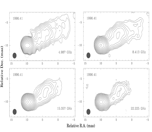
Figure 6: Special renditions of the maps of 3C 345 for epoch 1996.41 with a circular restoring beam of 1.2 mas diameter used to produce the spectral index maps shown in figure 7. The contours are 3 mJy$\times$(-1,1,1.73,3,…,). The peaks of brightness are of 3.69, 4.24, 4.30, and 3.05 Jy/beam respectively at 5, 8.4, 15, and 22 GHz. The shift of (10,-10 mas) with respect to the maps of Fig. 1 was made to reduce map sizes by computing reasons (the shift is unimportant as relative right ascension and declination are shown). Epochs 1995.84 and 1996.81 show similar features.

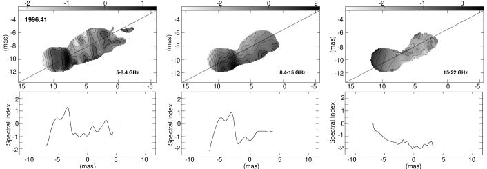
Figure 7: Spectral index maps (top in every subimage) and profiles (bottom) among the maps convolved with a 1.2 mas circular restoring beam (Fig. 6) from our multifrequency data set at 1996.41. The profile line follows the diagonal line over the maps, with a P.A. of 117^∘.

The registration of the images was done by considering the relative separations of the model fit components from the core (assuming that the components are optically thin), the theoretical predictions for the core registration (see Lobanov 1998a ), and the alignment of the jet components directly in the images.

In the spectral index maps, two different regions in the parsec-scale structure of 3C 345 are evident. The D/C8/C7 region is optically thick. The region of the more extended jet from about $\geq 1.5$ mas out of the core to the NW (P.A. $\sim-70^{\circ}$) is optically thin. The transition between both areas is located to the west of the component C7.

The core region displays spectral indices that allow one to deduce that the turnover frequency at this region is above 15 GHz, peaking between the core and C8, and decreasing to the west. The component trajectories obtained exhibit apparent proper motions of 0.2–0.3 mas/yr. The peaks of the spectral images are consistent with a shock evolution. This behavior and the shock parameters have been studied in detail by Lobanov & Zensus (lob99 (1999)) for previous observing epochs.

In the comparison of data sets of 5/8.4 and 15/22 GHz we find a gradient of the spectral index, increasing to the south: the southern edge of the jet is optically thicker than the northern edge. This has been observed at all three epochs, and we reject the possibility of a registration error after a careful test of different shift values. In the maps at 22 GHz, we observe a steeper fall in the flux density from the components to the south than to the north. There is some extended emission in this northern region. These gradients can be interpreted as an effect arising from changes in the speeds across the jet flow. The curved trajectories of the components can also be related to this effect.

At larger distances along the parsec-scale jet ($>$1.5mas), the spectrum shows an optically thin region, with the spectral index decreasing, becoming as steep as $\alpha_{\rm 22\,GHz}^{\rm 15\,GHz}\sim-2$. The peaks in the maps that include 5 GHz information can also be affected by beam overresolution. A similar gradient to the south is also evident in this region in most of the cases. There seems to be an intrinsic asymmetry in the jet, as we will also see in the polarization analysis, in Sect. 3.3. For a helical jet geometry (e.g., Villata & Raiteri vil99 (1999)) this intrinsic asymmetry can be explained by the beaming of emission towards the observer for one side of the helix —the southern in our case, and fainter emission in the other side.

In summary, the spectral behavior of the jet shows a scenario with a clear transition between two zones with different physical properties: the core region and the outer parsec-scale jet region. The components in the latter show a slower flux decrease than in the inner region (comparing the values in the model fit), and also higher speeds of the component proper motions.

3.3 Polarimetric imaging

Before discussing the VLBI results, we want to point out some facts observed in the single-dish monitoring results of the polarized emission of 3C 345. In Fig. 8, we plot the degree of polarization $m$ and the EVPA $\chi$ from the UMRAO data at epochs close to our observations.

Figure 8: Single dish $m$ and $\chi$ of 3C 345 (UMRAO).

The polarization angle of the total emission $\chi$ shows a value of $\sim 40^{\circ}$ close to 1995.84 and is constant around $\sim 20^{\circ}$ after early 1996. At higher frequencies, $\chi$ changes, showing a decrease and a further increase in its value. $\chi^{\rm UMRAO}_{\rm 15\,GHz}$ changes from values of $\sim 10^{\circ}$ at 1995.8 to $\sim-40^{\circ}$ in 1996.6, turning back to $\sim 20^{\circ}$ on early 1997. The degree of polarization remains between 1–2% during our three observing epochs. Interestingly, it increases up to 4% after our last VLBI observations in 1997.1, when the values $\chi$ at the three frequencies coincide again. This is the epoch where the C9 component appears in our model fitting, and also when the flux density begins to increase at the higher frequencies.

We can assume that the single dish polarization measurements of 3C 345 are almost equivalent to integrating all of the parsec-scale jet polarized components. The VLA polarized images mentioned above are consistent also with the single-dish measurements. At the epoch of 1995.8, $\chi^{\rm VLA}_{\rm 15\,GHz}\sim 5^{\circ}$, and $\chi^{\rm VLA}_{\rm 22\,GHz}\sim-10^{\circ}$.

In Fig. 9, we show the composition of the total intensity $I$ (contours), the polarized intensity $p$ (grey scale) and the electric vector orientation angle $\chi$ (segments, length proportional to $p$) for the observations in 1995.84 at 22 GHz. It is obvious that the electric vector is aligned with the extremely curved jet direction in the inner 3 mas.

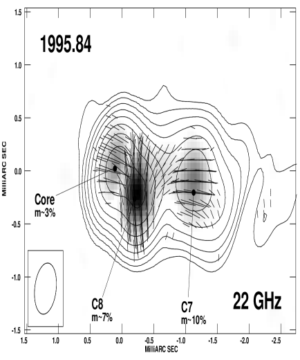
Figure 9: VLBA $I$, $p$ and $\chi$ images of 3C 345 at 22 GHz, epoch 1995.84. The total intensity $I$ is represented with contours (value of 6 mJy/beam$\times\,-1,1,2.24,5,11.18,25,\dots)$, superimposed over a grey scale polarized intensity map (peak of brightness of 112.4 mJy) and the superimposed electric vectors ($\chi$, length proportional to $p$, 1 mas in the map is equivalent to 100 mJy/beam).

Fig. 10 shows the total and polarized flux density for the three epochs along two cuts through the core, which are oriented at P.A. of 60^∘ and 90^∘, which cross, respectively, the components C8 and C7. The evolution of the total flux for the core D and components C8 and C7 is evident in the figure. The brightness peak of the polarized emission moves westwards, and a new component appears in 1996.81. The evolution of C8 is the most dramatic: in 1995.84, it dominates the $p$-map, then it becomes much weaker in 1996.41 and vanishes in 1996.81. The polarization angle of C8 rotates from the 1st to the 2nd epoch. The component C7 shows a westward motion, similar in total and polarized emission. The value of $\chi$ for this component is nearly constant throughout the period of observations. We can compare those results with the 22 GHz map from 3C 345 at epoch 1994.45 presented in Leppänen et al. (lep95 (1995)), 1.39 yr before our first epoch. Component C8 had emerged and was clearly visible in the polarization map, but not in the total intensity image. Its EVPA began to be oblique with respect to the values of D and C7, which were parallel to the jet, as it is observed also in our data. Our maps at 22 GHz represent a later stage in the evolution of the C8 component, which is rotating through its evolution.

Figure 10: Logarithmic slice profile of the total and polarized flux density maps of 3C 345 at 22 GHz through the core and the C8 (top) and C7 (bottom) components, crossing the center of the maps with a P.A. 60^∘and 90^∘, respectively (shown at the top left of each figure). The motion of the components in total intensity can be appreciated, and also the changes in the polarized flux density features.

Gómez et al. (gom94 (1994)) have modeled features similar to C8 from simulations of the emission in a bent shocked relativistic jet, reporting anticorrelation between the polarized and the total intensity emission, which is observed at early stages of evolution of a relativistic shock. We should point out that a possible superposition between components with different electric vector orientations may lead to cancellation of the polarized flux and can produce apparent gaps between polarized emission components. The brighter polarized emission in C8 might be explained by a shock wave in a curved jet. More generally, the features in Fig. 9 can be explained in terms of the shock model (Wardle et al. war94 (1994)) in the framework of a helical geometry for the motion of the components (Steffen et al. ste95 (1995), Villata & Raiteri vil99 (1999)). Lister et al. (lis98 (1998)) report similar vector alignment with the jet at 43 GHz, for the inner jet regions in several blazars.

In Fig. 11, we display the images of polarized emission in 3C 345 at 15 and 8.4 GHz, following the same scheme as in Fig. 9. The same features seen at 22 GHz are present here. At 8.4 GHz, weak polarized emission is also detected in the outer jet, at the northern edge, with $\chi\sim 0^{\circ}$. This change of the electric vector, roughly parallel to the jet direction at D and C7 contrasts with its value roughly perpendicular to it at the edge of the outer jet. The spectral analyses have shown that the jet at distances $>$1.5 mas of the core is an optically thin region, where also a north-south gradient in $\alpha$ was present.

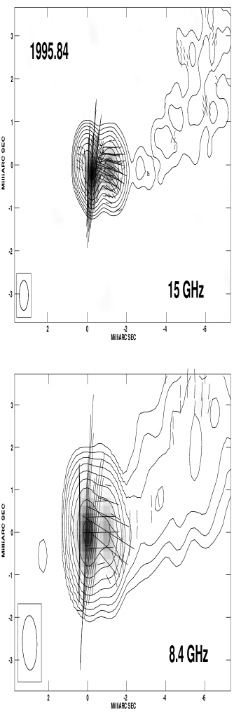
Figure 11: VLBA $I$, $p$ and $\chi$ images of 3C 345 at 15 and 8.4 GHz, epoch 1995.84. The total intensity $I$ is represented with contours (value of 6 mJy/beam$\times\,-1,1,2.24,5,11.18,25,\dots$), over a grey scale polarized intensity map (peaks of brightness of 169.3 and 141.4 mJy/beam, respectively, grey scale normalized to the common maximum polarized flux density –at 15 GHz–), and the electric vectors ($\chi$, length proportional to $p$, 1 mas in the map is equivalent to 50 mJy/beam).

At 5 GHz, the distribution of the polarized emission differs significantly from that seen at higher frequencies. In Fig. 12, we present the image obtained for the 3rd epoch of our monitoring. The two earlier epochs display very similar features in the jet. The core is less polarized ($m\sim 1\%$) than at higher frequencies, with its electric vector oblique to the jet direction. Both facts may be caused by the blending of two or more emission regions with different polarization angles. The degree of polarization at 5 GHz in the jet reaches $\sim$15%. The predominance of the polarized emission at the jet edges (especially at the northern one) is more obvious here than at 8.4 GHz.

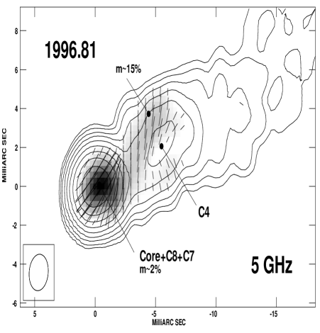
Figure 12: Polarized intensity electric vectors ($\chi$, length proportional to $p$, 1 mas in the map is equivalent to 10 mJy/beam) overlaid on total intensity ($I$) contours (3 mJy/beam$\times\,-1,1,2.24,5,11.18,25,...$) and grey scale polarized intensity ($p$, grey scale up to the peak of brightness, 40.5 mJy/beam) images for 3C 345 at 5 GHz, epoch 1996.81. It is obvious that the electric vector is almost perpendicular to the jet at core separations from 3 to 7 mas.

These findings seem to be consistent with the conclusions of Brown et al. (bro94 (1994)), who reported, at 5 GHz, a weakly polarized core in 3C 345 and a fractional polarization reaching 15% in the jet. The electric vector position angles were found to be variable in the core from one epoch to the other but perpendicular to the jet for all epochs. VLBA observations of 3C 345 at 8.4 GHz made in 1997.07 (Taylor tay98 (1998)) yield an image that is very similar to our image at 1996.81, and both images imply a magnetic field aligned with the jet direction at 3–10 mas distances from the core. Cawthorne et al. (caw93 (1993)) suggested that the longitudinal component of the magnetic field can increase with the distance from the core as a result of shear from the dense emission line gas near the nucleus. At larger distances from the core the shocks may become too weak to dominate the emission, resulting in the observed electric field perpendicular to the jet. This is possibly the physical mechanism that can explain the phenomena observed in our maps.

We also investigated the possible existence of a differential rotation measure (RM) at the edges of the outer jet, comparing cuts across the jet at 5 GHz and 8.4 GHz. Such a RM would be caused by a toroidal magnetic field (shear-like) in the jet (see Gabuzda gab99 (1999)). Owing to the uncertainties in $\chi$, the only reliable result is that the values of the EVPA are $\sim 40^{\circ}$ bigger in the southern than in the northern edge, both at 5 and at 8.4 GHz. No conclusions about the presence of this RM can be extracted.

4 Summary

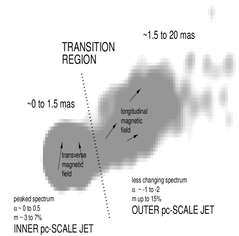
Figure 13: Summary of physical properties observed in the two regions of the parsec-scale jet of 3C 345. The values for $\alpha$ and $m$ refer to our four observing frequencies (5, 8.4, 15, and 22 GHz), in general.

We have observed the superluminal QSO 3C 345 with VLBI at three epochs within one year, observing with the VLBA at four frequencies. Our results quantify the superluminal motions of components C8 and C7 with respect to the core component D, and they show a remarkably complex polarization structure near the core, which provides evidence for emerging components and changing projected jet direction within 3 mas from the core. A comparison of our total intensity data at the four frequencies with previous model fitting results will provide a better understanding of the kinematical properties of the jet.

Spatial blending may be partly responsible for the low core polarization observed for quasars in centimeter VLBI polarimetry. Roberts et al. (rob87 (1987)) mention the possible interference between components with different $\chi$ in the polarized intensity for the case of OJ 287 at 5 GHz. Similar features can be present for the case of 3C 345, especially at 5 GHz, since different components have different values of $\chi$ at higher frequencies.

The polarized intensity images show alignment between the jet direction and the electric vector position angle in the inner regions of the jet at high frequencies, and orthogonality of the electric vector and the jet direction in the outer regions of the jet. These results are fully consistent with the previously reported observations of Brown et al. (bro94 (1994)), Leppänen et al. (lep95 (1995)), Taylor (tay98 (1998)), covering different frequencies and jet regions in 3C 345.

The interpretation of Lobanov & Zensus (lob96b (1996)) about a transition in the jet can be confirmed with the scenario provided by our observations (see Fig. 13). The core region (up to 1.5 mas), which presents magnetic field orientations predominantly transverse (Figs. 9 & 11), would be dominated by strong shocks (as components C8 and C7). This shock dominance is also consistent with the peaked spectrum (Fig. 7). At larger distances (beyond 1.5 mas), the trajectories of the components are less curved than in the inner jet and show faster speeds, the magnetic field is longitudinal (Fig. 12) and the spectrum is smoother (Fig. 7).

The jet in 3C 345, thus, apparently manifests different behaviors of the magnetic field, which can be explained in terms of different mechanisms: (i) magnetic field compression in the shocked, inner jet, (ii) ordering of the magnetic field in a shear layer and edge-brightened polarized emission in the outer jet, (iii) decoupling of two fluids within the jet with different properties, obliqueness of shocks interacting with the outer edge of the jet (C8), etc. To disentangle the different physical phenomena that are present in the jet, further observations are needed, with the goal of higher resolution, and including polarimetry. The VSOP facility and the use of mm-VLBI will provide important clues to the innermost structures of the radio source (Klare et al. in preparation). Continuing the multi-band monitoring of 3C 345 with VLBI, enhanced by regular polarimetric studies, and also observations at higher frequencies and with better resolution (like those provided by orbital VLBI results with HALCA) should help to better constrain the models of this QSO.

- (1) Aller H.D., Aller M.F., Hughes P.A., 1996, In: Miller R., Webb J.R., Noble J.C. (eds), Blazar Continuum Variability, ASP 110, San Francisco, CA, US, p. 208
- (2) Bartel N., Herring T.A., Ratner M.I., Shapiro I.I., Corey B.E., 1986, Nature 319, 733
- (3) Biretta J.A., Moore R.L., Cohen M.H., 1986, ApJ 308, 93
- (4) Brown L.F., Roberts D.H., Wardle J.F.C., 1994, ApJ 437, 108
- (5) Cawthorne T.V., Wardle J.F.C., Roberts D.H., Gabuzda D.C., 1993, ApJ 416, 519
- (6) Cotton W.D., Geldzahler B.J., Marcaide J.M., Shapiro I.I., Rius A., 1984, ApJ 286, 503
- (7) Gabuzda D.C., 1999, New Astronomy Reviews 43, 691
- (8) Gómez J.L., Alberdi A., Marcaide J.M., Marscher A.P., Travis J.P., 1994, A&A 292, 33
- (9) Hummel C.A., Schalinski C.J., Krichbaum T.P., et al., 1992, A&A 257, 489
- (10) Kollgaard R.I., Wardle J.F.C., Roberts D.H., 1989, AJ 97, 155
- (11) Leppänen K.J., Zensus J.A., Diamond P.J., 1995, AJ 110, 2479
- (12) Lister M.L., Marscher A.P., Gear W.R., 1998, ApJ 504, 702
- (13) Lobanov A.P., 1996, “Physics of the Parsec-Scale Structures in the Quasar 3C 345”, PhD Thesis, New Mexico Institute of Mining & Technology, Socorro, NM, US
- (14) Lobanov A.P., 1998a, A&A 330, 79
- (15) Lobanov A.P., 1998b, A&AS 132, 261
- (16) Lobanov A.P., Zensus J.A., 1996, In: Hardee P.E., Bridle A.H., Zensus J.A. (eds), Energy Transport in Radio Galaxies and Quasars, ASP 100, San Francisco, CA, US, p. 109
- (17) Lobanov A.P., Zensus J.A., 1999, ApJ 521, 509
- (18) Marziani P., Sulentic J.W., Dultzin-Hacyan D., Calvani M., Moles M., 1996, ApJS 104, 37
- (19) Pearson T.J., Readhead A.C.S., 1988, AJ 328, 114
- (20) Qian S.J., Krichbaum T.P., Zensus J.A., Steffen W., Witzel A., 1996, A&A 308, 395
- (21) Rantakyrö F.T., Bååth L.B., Matveenko L., 1995, A&A 293, 44
- (22) Roberts D.H., Gabuzda D.C., Wardle J.F.C., 1987, ApJ 323, 536
- (23) Romney J.D., 1985, VLBA Memo No. 452, NRAO, NM, US
- (24) Shepherd M.C., Pearson T.J., Taylor G.B., 1994, BAAS 26, 987
- (25) Steffen W., Zensus J.A., Krichbaum T.P., Witzel A., Qian S.J., 1995, A&A 302, 335
- (26) Taylor G.B., 1998, ApJ 506, 637
- (27) Teräsranta H., Tornikoski M., Mujunen A., et al., 1998, A&AS 132, 305
- (28) Türler M., Courvoisier T.J.-L., Paltani S., 1999, A&A 349, 45
- (29) Unwin S.C., Cohen M.H., Pearson T.J., et al., 1983, ApJ 271, 536
- (30) Villata M., Raiteri C.M., 1999, A&A 347, 30
- (31) Wardle J.F.C., Cawthorne T.V., Roberts D.H., Brown L.F., 1994, ApJ 437, 122
- (32) Zensus J.A., Cohen M.H., Unwin S.C., 1995a, ApJ 443, 35
- (33) Zensus J.A., Krichbaum T.P., Lobanov A.P., 1995b, Proc. Natl. Acad. Sci. USA 92, 11348
- (34) Zhang X., Xie G.Z., Bai J.M., 1998, A&A 330, 469