On the conversion of blast wave energy into radiation in active galactic nuclei and gamma-ray bursts

Abstract

It has been suggested that relativistic blast waves may power the jets of AGN and gamma-ray bursts (GRB). We address the important issue how the kinetic energy of collimated blast waves is converted into radiation. It is shown that swept-up ambient matter is quickly isotropised in the blast wave frame by a relativistic two-stream instability, which provides relativistic particles in the jet without invoking any acceleration process. The fate of the blast wave and the spectral evolution of the emission of the energetic particles is therefore solely determined by the initial conditions. We compare our model with existing multiwavelength data of AGN and find remarkable agreement.

1 Introduction

Shortly after the detection of more than 60 blazar-type active galaxies as emitters of MeV–GeV $\gamma$-rays by EGRET on board the Compton Gamma-Ray Observatory (CGRO) (von Montigny et al. cvm95 (1995), Mukherjee et al. muk97 (1997)), observations with ground-based Čerenkov telescopes have shown that at least for BL Lacertae objects the $\gamma$-ray spectrum can be traced to more than a TeV observed photon energy (Punch et al. pun92 (1992), Quinn et al. qui96 (1996), Catanese et al. cat98 (1998), Krennrich et al. kre97 (1997)). In these sources the bulk of luminosity is often emitted in the form of $\gamma$-rays. The typical $\gamma$-ray spectra of blazars are well described by power laws in the energy range between a few MeV and a few GeV (Mukherjee et al. muk97 (1997)), but display a break around an MeV (McNaron-Brown et al. mnb95 (1995)). At GeV energies the spectra show a tendency of getting harder during outbursts (Pohl et al. poh97 (1997)). The $\gamma$-ray emission of the typical blazar is highly variable on all timescales down to the observational limits of days at GeV energies and hours at TeV energies (e.g. Mattox et al. mat97 (1997), Gaidos et al. gai96 (1996)). Large amplitude variability at TeV energies is generally not associated with corresponding variability at GeV energies (Lin et al. lin94 (1994), Buckley et al. buc96 (1996)).

Correlated monitoring of the sources at lower frequencies has demonstrated that $\gamma$-ray outbursts are accompanied by activity in the optical and radio band (Reich et al. rei93 (1993), Mücke et al. mue96 (1996), Wagner wag96 (1996)). Emission constraints such as the compactness limit and the Elliot-Shapiro relation (Elliot & Shapiro es74 (1974)) are violated in some $\gamma$-ray blazars, even when these limits are calculated in the Klein-Nishina limit (Pohl et al. poh95 (1995), Dermer & Gehrels dg95 (1995)), which implies relativistic bulk motion within the sources. This conclusion is further supported by observations of apparent superluminal motion in many $\gamma$-ray blazars (e.g. Pohl et al. poh95 (1995), Barthel et al. bar95 (1995), Piner & Kingham 1997a ; 1997b ).

Published models for the $\gamma$-ray emission of blazars are usually based on inverse Compton scattering of soft target photons by highly relativistic electrons in the jets of these sources. The target photons may come directly from an accretion disk (Dermer et al. dsm92 (1992), Dermer & Schlickeiser ds93 (1993)), or may be rescattered accretions disk emission (Sikora et al. sbr94 (1994)), or may be produced in the jet itself via synchrotron radiation (e.g. Bloom & Marscher bm93 (1996) and references therein). In all the above models the jet and its environment is assumed to be optically thin for $\gamma$-rays in the MeV–GeV range. A common property of the inverse Compton models is the emphasis on the radiation process and the temporal evolution of the electron spectrum and the neglect of the problem of electron injection and acceleration (for an exception see Blandford & Levinson bl95 (1995)). The modeling of the multifrequency spectra of blazars often requires a low energy cut-off in the electron injection spectrum, but no high energy cut-off. The usual shock or stochastic electron acceleration processes would have to be very fast to compete efficiently with the radiative losses at high electron energies, and a high energy cut-off should occur under realistic conditions, but no low energy cut-off (e.g. Schlickeiser sch84 (1984)), in contrast to the requirements of the spectral modeling.

When efficient, but possibly slower, acceleration of protons is assumed, photomeson production on ambient target photons can provide many secondary electrons and positrons with a spectrum as required by the multifrequency modeling (Kazanas & Ellison ke86 (1986), Sikora et al. sik87 (1987), Mannheim & Biermann mb92 (1992)). Such systems are usually optically thick and a pair cascade develops. In these models multi-TeV $\gamma$-ray emission can be easily produced, but the observed short variability timescale places extreme constraints on the magnetic field strength, because the proton gyroradius has to be much smaller than the system itself, and on the Doppler factor, because the intrinsic timescale for switching off the cascade is linked to the observed soft photon flux via the energy loss rate for photomeson production. For the most rapid $\gamma$-ray outburst of Mrk 421 (Gaidos et al. gai96 (1996)) this leads to $B\gg 10\ {\rm G}$ and $D\gg 100$.

Another class of models features hadronic collisions of a collimated proton jet with BLR clouds entering the jet (e.g. Dar & Laor dl97 (1997); Beall & Bednarek bb99 (1999)). These models have two theoretical difficulties: the proton beam is weak compared with the background plasma and therefore quickly stopped by a two-stream instability. Also the BLR clouds are usually optically thick and thus the efficiency of the system is drastically reduced.

In this paper we consider a strong electron-proton beam that sweeps up ambient matter and thus becomes energized. The basic scenario is similar to the blast wave model for $\gamma$-ray bursts (GRBs) which successfuly explains the time dependence of the X-ray, optical and radio afterglows (e.g. Wijers et al. wmr97 (1997), Vietri 1997a , Waxman 1997a ). There the apparent release of $\simeq 10^{52}E_{52}$ erg of energy in a small volume leads to the formation of a relativistically expanding pair fireball that transforms most of the explosion energy into kinetic energy of baryons in a relativistic blast wave. We assume that a similar generation process also powers the relativistic outflows in active galactic nuclei (AGN), but that the outflow is not spherically symmetric and highly channelled along magnetic flux tubes into a small fraction of the full solid angle due to the structure of the medium surrounding the point of energy release.

We shall address the important issue how the kinetic energy of such channelled relativistic blast waves is converted into radiation. Existing radiation modelling of GRBs and AGNs (see e.g. Vietri 1997b ; Waxman 1997b ; Böttcher & Dermer bd98 (1998)) are very unspecific on this crucial point. Typically it is assumed that a fraction $\xi$ of the energy in nonthermal baryons in the blast wave region at position $x$ is transformed into a power-law distribution of ultrarelativistic cosmic ray protons with Lorentz factors $\Gamma(x)\leq\gamma_{\rm CR}\leq\gamma_{\rm max}$ in the fluid frame comoving with a small element of the blast wave region that travels with the bulk Lorentz factor $\Gamma(x)=\Gamma_{0}(x/x_{0})^{-g}$ after the deceleration radius $x_{0}=2.6\cdot 10^{16}(E_{52}/n_{0}\Gamma_{0,300}^{2})^{1/3}$ cm through the surrounding medium of density $n_{0}$. For electrons it is argued (Katz & Piran kp97 (1997), Panaitescu & Mészáros pm98 (1998)) that their minimum Lorentz factor is $\gamma_{\rm e,min}=(m_{\rm p}/m_{\rm e})\Gamma$ since they are in energy equilibrium with the protons. Here we investigate this transfer mechanism from the channelled blast wave to relativistic protons and electrons in more detail. In Sect. 2 we consider the penetration of a blast wave consisting of cold protons and electrons with density $n_{\rm b}$ with the surrounding ”interstellar” medium consisting also of cold protons and electrons on the basis of a two-stream instability. Viewed from the coordinate system comoving with the blast wave, the interstellar protons and electrons represent a proton-electron beam propagating with the relativistic speed $V(x)=-c(1-\Gamma^{-2}(x))^{1/2}$ antiparallel to the $x$-axis. We examine the stability of this beam assuming that the background magnetic field is uniform and directed along the x-axis. We demonstrate that very quickly the beam excites low-frequency magnetohydrodynamic plasma waves, mainly Alfvén-ion-cyclotron and Alfvén-Whistler waves. These plasma waves quasi-linearly isotropise the incoming interstellar protons and electrons in the blast wave plasma. In Sect. 3 we investigate the interaction processes of these isotropised protons and electrons (hereafter referred to as primary protons and electrons), which have the relativistic Lorentz factor $\Gamma(x)$, with the blast wave protons and electrons. Since the primary protons carry much more momentum than the primary electrons, inelastic collisions between primary protons and the blast wave protons generate neutral and charged pions which decay into gamma rays, secondary electrons, positrons and neutrinos. Both, the radiation products from these interactions, and the resulting cooling of the primary particles in the blast wave plasma, are calculated. By transforming to the laboratory frame we calculate the time evolution of the emitted multiwavelength spectrum for an outside observer under different viewing angles. Momentum conservation leads to a deceleration of the blast wave that is taken into account self-consistently. Since we do not consider any re-acceleration of particles in the blast wave, the evolution of particles and the blast wave is completely determined by the initial conditions.

2 Two-stream instability of a proton-electron beam

2.1 Physical model and basic equations

As sketched in Fig. 1 we consider in the laboratory frame (all physical quantities in this system are indexed with $*$) the cold blast wave electron-proton plasma of density $n^{*}_{\rm b}$ and thickness $d^{*}$ in $x$-direction running into the cold interstellar medium of density $n^{*}_{0}$, consisting also of electrons and protons, parallel to the uniform magnetic field of strength $B$. In the comoving frame the total phase space distribution function of the plasma in the blast wave region at the start thus is

$$f^{*}(\@vec{p}^{*},t=0)= {1\over 2\pi p_{\perp}^{*}}n^{*}_{0}\delta\bigl{(}p^{*}_{\perp}\bigr{)}\delta\bigl{(}p^{*}_{\parallel}\bigr{)}$$ (1)

$$+ {1\over 2\pi p_{\perp}^{*}}n^{*}_{\rm b}\delta\bigl{(}p^{*}_{\perp}\bigr{)}\delta\bigl{(}p^{*}_{\parallel}-P\bigr{)},$$

where

$$P=\Gamma mV=\Gamma m\beta c=mc\sqrt{\Gamma^{2}-1)}.$$

The Lorentz transformations (e.g. Hagedorn hag73 (1963), p.41) to the blast wave rest frame with momentum and energy variables $(p_{\perp},p_{\parallel},E)$ are

$$p^{*}_{\perp}=p_{\perp},\;\;\;p^{*}_{\parallel}=\Gamma(p_{\parallel}+\,\beta{E\over c}),\;\;\;E^{*}=\Gamma(E+\,\beta cp_{\parallel})\ .$$ (2)

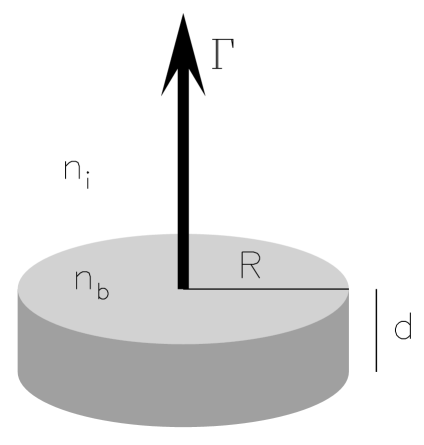
Figure 1: Sketch of the basic geometry. The thickness of the channeled blast wave $d$, measured in its rest frame, is much smaller than its halfdiameter. The blast wave moves with a bulk Lorentz factor $\Gamma$ through ambient matter of density $n_{\rm i}$.

Using the invariance of the phase space densities we obtain for the phase space density in the blast wave rest frame

$$f(\@vec{p},t=0) = f^{*}(\@vec{p}^{*}(\@vec{p}),t=0)$$ (3)

$$= {{n_{\rm i}\delta\bigl{(}p_{\perp}\bigr{)}\delta\bigl{(}p_{\parallel}-P\bigr{)}}\over{2\pi p_{\perp}}}+\;{{n_{\rm b}\delta\bigl{(}p_{\perp}\bigr{)}\delta\bigl{(}p_{\parallel}\bigr{)}}\over{2\pi p_{\perp}}}\ ,$$

where the number densities are

$$n_{\rm i}=\Gamma n_{0}^{*},\;\;\,n_{\rm b}=n_{\rm b}^{*}/\Gamma\ .$$

The blast wave density transformation is inverse to that for the density of interstellar matter because of the different rest systems.

In terms of spherical momentum coordinates $p_{\parallel}=p\mu$ and $p_{\perp}=p\sqrt{1-\mu^{2}}$ the distribution function (3) reads

$$f({p},t=0) = {1\over 2\pi p^{2}}n_{\rm i}\delta\bigl{(}\mu+1\bigr{)}\delta\bigl{(}p-P\bigr{)}+\;{1\over 4\pi p^{2}}n_{\rm b}\delta\bigl{(}p\bigr{)}$$ (4)

$$= n_{\rm b}f_{\rm b}(p,\mu,t=0)+\,n_{\rm i}f_{i}(p,\mu,t)\ ,$$

where $\mu=p_{\parallel}/p$ is the cosine of the pitch-angle of the particles in the magnetic field $B$ pointing to positive $z$-direction. Obviously, the incoming interstellar protons and electrons are a beam propagating antiparallel to the magnetic field direction in the blast wave plasma. For ease of exposition we assume that the blast wave plasma is cold, i.e. $f_{\rm b}\propto\delta(p)$.

The blast wave density $n^{*}_{\rm b}=10^{8}n^{*}_{\rm b,8}$ is much larger than the interstellar gas density $n^{*}_{0}=1n^{*}_{\rm i}$. We want to calculate the time $t_{\rm R}$ it takes to isotropise the incoming interstellar protons and electrons; if this relaxation time is much smaller than $d/c$ an isotropic distribution of primary protons and electrons is effectively generated.

If the beam distribution function $f_{i}$ in Eq. (4) is unstable in the blast wave plasma it will excite plasma waves. Therefore we have to find the dispersion relation $\omega=\omega(k)$ which are perturbations of the form

$$\delta\@vec{E}=\delta\@vec{E}_{0}\,\exp(\imath(\@vec{k}\cdot\@vec{x}-\omega t))\ .$$ (5)

It has been shown (Kennel & Wong kw67 (1967), Tademaru tad69 (1969)) that waves propagating obliquely to the magnetic field are thermally damped by the background (=blast wave) plasma, so that we concentrate on parallel ($\@vec{k}||\@vec{B}$) waves. One finds two implicit dispersion relations (Baldwin et al. bbw69 (1969); Achatz et al. asl90 (1990)), one for electrostatic waves $(\delta\@vec{E}||\@vec{B})$

$$0=\omega^{2}-\;\omega_{\rm p,p}^{2}-\;\omega_{\rm p,e}^{2}-\;{n_{\rm i}\over n_{\rm b}\Gamma^{3}}\left(1+{{m_{\rm e}}\over{m_{\rm p}}}\right){\omega_{\rm p,e}^{2}\omega^{2}\over[\omega+kV]^{2}}\ ,$$ (6)

and one for electromagnetic $(\delta\@vec{E}\perp\@vec{B})$

$${n_{\rm i}\omega_{\rm p,e}^{2}[\omega+kV]\over n_{\rm b}\Gamma}\,\bigl{[}[\omega+kV-{{\Omega_{\rm e}}\over{\Gamma}}]^{-1}+\;{{m_{\rm e}}\over{m_{\rm p}}}[\omega+kV-{{\Omega_{\rm p}}\over{\Gamma}}]^{-1}\bigr{]}\hfil$$

$$+\left[c^{2}k^{2}-\;\omega^{2}+\;{\omega\omega_{\rm p,p}^{2}\over\omega-\Omega_{\rm p}}+\;{\omega\omega_{\rm p,e}^{2}\over\omega-\Omega_{\rm e}}\right]=0\ ,\hfill$$ (7)

where $\omega_{\rm p,j}=\sqrt{4\pi n_{\rm b}q_{\rm j}^{2}/m_{\rm j}}$ denotes the plasma frequency and $\Omega_{\rm j}=q_{\rm j}B/m_{\rm j}c$ the nonrelativistic gyrofrequency of particle species $j$. In our notation negative (positive ) frequencies $\omega_{\rm R}$ refer to right-handed (left-handed) circularly polarised waves, respectively. Moreover, positive phase speeds $(\omega_{\rm R}/k>0)$ indicate forward propagating waves and negative phase speeds $(\omega_{\rm R}/k<0)$ backward propagating waves. Here we will concentrate on the excitation of the electromagnetic waves. The excitation of electrostatic turbulence and its backreaction on the particle distribution function will be discussed in a forthcoming publication. Because

$$n_{\rm i}/n_{\rm b}=\Gamma^{2}n^{*}_{0}/n^{*}_{\rm b}=10^{-4}\Gamma_{100}^{2}n_{\rm i}^{*}/n^{*}_{\rm b,8}<<1\ ,$$ (8)

the beam is weak and the contributions from the beam in Eq.(7) can be described as perturbations to the dispersion relation in a single component electron-proton plasma ($n_{\rm i}=0$). Its solutions

$$c^{2}k^{2}=J(\omega_{\rm R})\equiv\omega_{\rm R}^{2}\Bigl{(}1+\;{\omega_{\rm p,e}^{2}\over\Omega_{\rm e}^{2}}+\;{\omega_{\rm p,e}^{2}\over(\omega_{\rm R}-\Omega_{\rm p})\Omega_{\rm e}}\Bigr{)}\$$ (9)

are

(a) Alfvén waves

$$\omega_{R}^{2}=V_{\rm A}^{2}k^{2}\$$ (10)

at frequencies $|\omega_{\rm R}|<<\Omega_{\rm p}$, where $V_{\rm A}=B(4\pi m_{\rm p}n_{\rm b})^{-1/2}$ is the Alfvén speed and $\omega_{\rm R}=\Re(\omega)$. The dispersion relation (10) accounts for four types of Alfvén waves: forward and backward moving, right-handed and left-handed polarised;

(b) Whistler waves

$$\omega_{\rm R}=\Omega_{\rm e}k^{2}c^{2}/\omega_{\rm p,e}^{2}\$$ (11)

at frequencies between $\Omega_{\rm e}<\omega_{\rm R}<-\Omega_{\rm p}$. The dispersion relation (11) describes right-handed polarised waves (because $\Omega_{\rm e}<0$) that propagate forward for negative $k<0$ and backward for positive $k>0$.

All of these are stable ($\psi=\Im(\omega)=0$) if the beam particles are absent. As is explained in Achatz et al. (asl90 (1990)) the beam protons and electrons, which under the given weak-beam condition do not affect each other, are however able to trigger each its instability which occurs if the resonance conditions

$$\omega_{\rm R}=-kV+\;(\Omega_{\rm p}/\Gamma),\;\;\;\omega_{\rm R}=-kV+\;(\Omega_{\rm e}/\Gamma),\;\;\;$$ (12)

can be satisfied.

The time-dependent behaviour of the intensities $I(k,t)$ of the excited waves is given by (Lerche ler67 (1967), Lee & Ip li87 (1987))

$${\partial I_{\rm n}\over\partial t}=\psi_{\rm n}I_{\rm n}\ ,$$ (13)

where the growth rate $\psi$ is

$$\psi(k)\simeq\pi^{2}c^{3}[{\partial J(\omega_{\rm R})\over\partial\omega_{\rm R}}]^{-1}\rm{sgn}(k)\sum_{i}\omega_{p,i}^{2}(m_{i}c)^{3}\ \times$$

$$\int_{E_{i}}^{\infty}dE\ {{E^{2}-1-({E\over N}-x_{i})^{2}}\over\sqrt{E^{2}-1}}{\partial f_{i}\over\partial\mu}\delta(\mu+{{x_{i}}\over\sqrt{E^{2}-1}})\ ,$$ (14)

where $N=ck/\omega_{\rm R}$ is the index of refraction and further $E_{i}=\sqrt{1+x_{i}^{2}}$ whith $x_{i}=\Omega_{\rm i,0}/kc$.

To describe the influence of these excited waves on the beam particles we use the quasilinear Fokker-Planck equation (e.g. Schlickeiser sch89 (1989)) for the resonant wave-particle interaction. For Alfvén waves and for Whistler waves the index of refraction

$$|N_{\rm A}|={\sqrt{J(\omega_{\rm R})}\over|\omega_{\rm R}|}\simeq 1-{\omega_{\rm p,e}^{2}\over\Omega_{\rm e}\Omega_{\rm p}}\simeq(c/V_{\rm A})^{2}>>1$$ (15)

$$|N_{\rm W}|\simeq({\omega_{\rm p,e}\over\Omega_{\rm e}})^{2}>>1$$ (16)

is large compared to unity, so that the Lorentz force associated with the magnetic field of the waves is much larger than the force associated with the electric field, so that on the shortest time scale these waves scatter the particles in pitch angle $\mu$ but conserve their energy, i.e. they isotropise the beam particles. The Fokker-Planck equation for the phase space density then reads

$${\partial f_{i}\over\partial t}={\partial\over\partial\mu}\bigl{[}D_{\rm\mu\mu}{\partial f_{i}\over\partial\mu}\bigr{]}\ ,$$ (17)

where the pitch angle Fokker-Planck coefficient is determined by the wave intensities $I_{\rm n}$

$$D_{\rm\mu\mu}\simeq\sum_{n}{{\pi\,\Omega_{i}^{2}\,(1-\mu^{2})}\over{2\,B^{2}}}\int_{-\infty}^{\infty}dk\ I_{\rm n}(k)\,\delta(\omega_{\rm R}-kv\mu-\Omega_{i})$$

  (18)

Using the dispersion relation of Alfvén waves ($\omega_{\rm R}\simeq V_{\rm A}k$), Eq. (18) indicates that beam protons and electrons resonate with waves at wavenumbers given by the inverse of their Larmor radii times $\mu$, $k\simeq\Omega_{i}/\Gamma v\mu=(\mu R_{i})^{-1}$. For protons these wavenumbers correspond to Alfvén waves. For electrons these wavenumbers correspond to Alfvén waves if the bulk Lorentz factor is above $|\mu|(m_{\rm p}/m_{\rm e})=1836|\mu|$, and Whistler waves for smaller Lorentz factors. We concentrate here on the isotropisation by Alfvén waves mainly for two reasons:

(1) the bulk of the momentum of the inflowing interstellar particles is carried by the protons so that they are energetically more important than the electrons;

(2) for Lorentz factors $\Gamma>|\mu|m_{\rm p}/m_{\rm e}$ the isotropisation of electrons is also caused by scattering with Alfvén waves; for smaller Lorentzfactors the mistake one makes in representing the Whistler dispersion relation still by the Alfvén dispersion relation is relatively small.

2.2 Self excited Alfvén waves

For Alfvén waves (10) we obtain

$${\partial J(\omega_{\rm R})\over\partial\omega_{\rm R}}\simeq 2\omega_{\rm R}c^{2}/V_{\rm A}^{2}=2c^{2}k/V_{\rm A}$$ (19)

which is positive for forward ($k>0$) moving waves and negative for backward ($k<0$) moving waves. According to Eq. (14) we obtain for the growth rate of forward (+) and backward (-) moving Alfvén waves

$$\psi_{\rm\pm}=\pm\psi$$ (20)

with

$$\psi= {\pi^{2}V_{\rm A}\over c^{2}|k|}\sum_{i}\omega_{p,i}^{2}(m_{i}c)^{3}\ \times\$$ (21)

$$\int_{E_{i}}^{\infty}dE{E^{2}-E_{i}^{2}\over\sqrt{E^{2}-1}}{\partial f_{i}\over\partial\mu}\delta(\mu+x_{i}(E^{2}-1)^{-1/2})\$$

Now it is convenient to introduce the normalised phase space distribution function of the beam particles

$$f_{i}(p,\mu,t)={\delta(E-\Gamma)\over 2\pi(m_{i}c)^{3}\Gamma(\Gamma^{2}-1)^{1/2}}F_{i}(\mu,t)\ ,$$ (22)

where $E=\sqrt{1+(p/mc)^{2}}$, so that Eq. (21) reduces to

$$\psi= {\pi\over 2}{V_{\rm A}\over c^{2}|k|}\sum_{i}{\omega_{\rm p,i}^{2}\over\Gamma}H[\Gamma-\sqrt{1+x_{i}^{2}}][1-{x_{i}^{2}\over\Gamma^{2}-1}]\ \times\$$ (23)

$${\partial F_{i}\over\partial\mu}\delta(\mu-x_{i}(\Gamma^{2}-1)^{-1/2})\$$

where $H[x]=1(0)$ for $x>(<)0$ is the step function. Summing over protons and electrons separately, and introducing the proton and electron Larmor radii, $R_{\rm p}=c\sqrt{\Gamma^{2}-1}/\Omega_{\rm p}$, $R_{\rm e}=c\sqrt{\Gamma^{2}-1}/|\Omega_{\rm e}|$, respectively, Eq. (23) becomes

$$\psi=b(|k|)\sum_{\rm x=e,p}\$$

$${m_{\rm e}\over m_{x}}[1-(kR_{\rm x})^{-2}]H[|k|-R_{\rm x}^{-1}]{\partial F_{\rm x}\over\partial\mu}\delta(\mu+(R_{\rm x}k)^{-1})\qquad$$ (24)

with

$$b(|k|)\equiv{\pi\over 2}{V_{\rm A}\over c}{n_{\rm i}\over n_{\rm b}\Gamma}{\omega_{\rm p,e}^{2}\over c|k|}\ .$$ (25)

According to Eqs. (13) and (20) written in the form

$${\partial I_{+}(t)\over\partial t}=\psi I_{+}(t)\$$ (26)

$${\partial I_{-}(t)\over\partial t}=-\psi I_{-}(t)\$$ (27)

we derive

$${\partial(I_{+}(t)I_{-}(t))\over\partial t}=0\$$ (28)

and

$${\partial[I_{+}(t)-I_{-}(t)]\over\partial t}=\psi[I_{+}(t)+I_{-}(t)]\$$ (29)

or when integrated,

$$I_{+}(t)I_{-}(t)=I_{+}(t=0)I_{-}(t=0)\$$ (30)

and

$$[I_{+}(t)-I_{-}(t)]-[I_{+}(t=0)-I_{-}(t=0)]=Z(k)\$$ (31)

with

$$Z(k)\equiv b(|k|)\sum_{\rm x=e,p}{m_{\rm e}\over m_{\rm x}}[1-(kR_{\rm x})^{-2}]H[|k|-R_{\rm x}^{-1}]\ \times$$

$$\int_{0}^{t}dt^{{}^{\prime}}\,{\partial F_{\rm x}\over\partial\mu}\delta(\mu+(R_{\rm x}k)^{-1})\left(I_{+}(t^{{}^{\prime}})+I_{-}(t^{{}^{\prime}})\right)\quad$$ (32)

which relates the wave intensities of forward (+) and backward (-) moving waves at any time $t$ to the initial wave intensities at time $t=0$.

In terms of the normalised distribution functions (22) the proton and electron distribution functions evolve according to Eqs. (17)-(18),

$${\partial F_{\rm p}\over\partial t}={\partial\over\partial\mu}\bigl{[}a_{\rm p}(|\mu|)\sum_{\pm}I_{\pm}(|R_{\rm p}\mu|^{-1}){\partial F_{\rm p}\over\partial\mu}\bigr{]}\$$ (33)

$${\partial F_{\rm e}\over\partial t}={\partial\over\partial\mu}\bigl{[}a_{\rm e}(|\mu|)\sum_{\pm}I_{\pm}(|R_{\rm e}\mu|^{-1}){\partial F_{\rm e}\over\partial\mu}\bigr{]}\$$ (34)

with

$$a_{\rm p}(|\mu|)\equiv{\pi\over 2}{v(1-\mu^{2})\over B^{2}R_{\rm p}^{2}|\mu|},\;\;\;a_{\rm e}(|\mu|)\equiv{\pi\over 2}{v(1-\mu^{2})\over B^{2}R_{\rm e}^{2}|\mu|}\$$ (35)

Integrating Eqs. (33) and (34) over $t$ and $\mu$ gives because of $a_{\rm p,e}(\mu=-1)=0$

$$\int_{-1}^{\mu}d\mu^{{}^{\prime}}[F_{\rm p,e}(\mu^{{}^{\prime}},t)-F_{\rm p,e}(\mu^{{}^{\prime}},t=0)]$$

$$=a_{\rm p,e}(|\mu|)\sum_{\pm}\int_{0}^{t}dt^{{}^{\prime}}I_{\pm}(|R_{\rm p,e}\mu|^{-1},t^{{}^{\prime}}){\partial F_{\rm p,e}\over\partial\mu}\$$ (36)

respectively. Evaluating Eq. (36) at $\mu=-(R_{\rm p}k)^{-1}$ for protons and at $\mu=(R_{\rm e}k)^{-1}$ we obtain

$$\sum_{\pm}\int_{0}^{t}dt^{{}^{\prime}}I_{\pm}(|k|,t^{{}^{\prime}}){\partial F_{\rm p}\over\partial\mu}\delta(\mu+(R_{\rm p}k)^{-1})=$$

$$a_{\rm p}^{-1}(|R_{\rm p}k|^{-1})\int_{-1}^{-1/(R_{\rm p}k)}d\mu[F_{\rm p}(\mu,t)-F_{\rm p}(\mu,t=0)]\$$ (37)

and

$$\sum_{\pm}\int_{0}^{t}dt^{{}^{\prime}}I_{\pm}(|k|,t^{{}^{\prime}}){\partial F_{\rm e}\over\partial\mu}\delta(\mu-(R_{\rm e}k)^{-1})=$$

$$a_{\rm e}^{-1}(|R_{\rm e}k|^{-1})\int_{-1}^{1/R_{\rm e}k}d\mu[F_{\rm e}(\mu,t)-F_{\rm e}(\mu,t=0)]\$$ (38)

Eqs. (37) and (38) can be inserted in Eq. (32) yielding

$$Z(k)={m_{\rm e}\over m_{\rm p}}{b(|k|)\over a_{\rm p}(|R_{\rm p}k|^{-1})}[1-(kR_{\rm p})^{-2}]\ \times$$

$$\sum_{\rm x=e,p}H[|k|-R_{\rm x}^{-1}]\int_{-1}^{{-{\rm sgn}(\Omega_{\rm x,0})}\over{R_{\rm x}k}}d\mu\ [F_{\rm x}(\mu,t)-F_{\rm x}(\mu,0)]$$ (39)

The system of the coupled equations (30,31,32) and (39) describes the temporal development of the particle distribution functions $F_{\rm p}$ und $F_{\rm e}$ under the influence of self-excited Alfvén waves propagating either forward (+) or backward (-). Here the boundary conditions are as follows: in the beginning ($t=0$) there is the mono-energetic beam distribution (1), i.e. in terms of the normalised distribution (22)

$$F_{\rm p,e}(\mu,t=0)=\delta(\mu+1)\$$ (40)

The final state of the isotropisation phase is reached at time $T_{i}$ when both growth rate and temporal derivative of the distribution disappear, i.e. when $\partial F_{i}/\partial\mu=0$. Consequently

$$F_{\rm p,e}(\mu,t=T_{i})={1\over 2}$$ (41)

At this time the Alfvén waves have completely isotropised the beam distrution. In order to estimate this time scale $T_{i}$ or the associated isotropisation length $\lambda$ we consider the extreme case that the wave spectrum is constant and equals the wave intensity spectrum after the isotropisation. By this method an approximation of the pitch angle Fokker-Planck coefficient $D_{\rm\mu\mu}$ is possible so that one gets a strict lower limit to the isotropisation length $\lambda$. By demonstrating that this length is much smaller than the thickness $d$ of the blast wave region we will establish that the inflowing proton-electron-beam is effectively isotropised in the blast wave plasma.

Inserting Eqs. (40) and (41) we find with

$$\int_{-1}^{-1/R_{\rm p}k}d\mu[F_{\rm p}(\mu,T_{i})-F_{\rm p}(\mu,t=0)]=-{1\over 2}\bigl{(}1+{1\over R_{\rm p}k}\bigr{)}\$$ (42)

and

$$\int_{-1}^{1/R_{\rm e}k}d\mu[F_{\rm e}(\mu,T_{i})-F_{\rm e}(\mu,t=0)]=-{1\over 2}\bigl{(}1-{1\over R_{\rm e}k}\bigr{)}\$$ (43)

that Eq. (39) becomes

$$Z(k) = -{m_{\rm e}\over m_{\rm p}}{b(|k|)\over 2a_{\rm p}(|R_{\rm p}k|^{-1})}[1-(kR_{\rm p})^{-2}]\hfill\qquad$$ (44)

$$\times\sum_{\rm x=e,p}\,[1+(kR_{\rm x})^{-1}]H[|k|-R_{\rm x}^{-1}]\hfill\qquad$$

$$= -{m_{\rm e}\over m_{\rm p}}{V_{\rm A}\over 2v}{\omega_{\rm p,e}^{2}\over c^{2}k^{2}}B^{2}R_{\rm p}{n_{\rm i}\over n_{\rm b}\Gamma}\hfill\qquad$$

$$\times\sum_{\rm x=e,p}\,[1+(kR_{\rm x})^{-1}]H[|k|-R_{\rm x}^{-1}]\hfill\qquad$$

$$\simeq -Z_{0}k^{-2}$$

The general solution of Eqs. (30) and (31) at time $t=T_{i}$ is

$$I_{+}(T_{i})= \sqrt{Y+{1\over 4}(Z+I_{+}(0)-I_{-}(0))^{2}}$$ (45)

$$+0.5\,\left(Z+I_{+}(0)-I_{-}(0)\right)$$

$$I_{-}(T_{i})= \sqrt{Y+{1\over 4}(Z+I_{+}(0)-I_{-}(0))^{2}}$$ (46)

$$-0.5\,\left(Z+I_{+}(0)-I_{-}(0)\right)$$

where

$$Y\equiv I_{+}(0)I_{-}(0)$$ (47)

If the initial turbulence is much weaker than the self-generated turbulence $I(k,0)<<|Z(k)|$ and has a vanishing cross-helicity $I_{+}(k,0)=I_{-}(k,0)=I(k,0)$ we obtain for Eqs. (45,46,47) approximately

$$I_{\pm}(k,T_{i})\simeq{1\over 2}[|Z|\pm Z]+\;{I^{2}(k,0)\over|Z|}$$ (48)

According to Eq. (44) $Z(k)$ is negative so that Eq. (48) reduces to

$$I_{+}(k,T_{i})\simeq{I^{2}(k,0)\over|Z(k)|}$$ (49)

and

$$I_{-}(k,T_{i})\simeq|Z(k)|$$ (50)

i.e. the beam mainly generates backward moving Alfvén waves in the blast wave plasma.

2.3 Energy budget

The total enhancement in magnetic field fluctuation power due to proton and electron isotropisation is obtained by integrating Eq. (31) using Eq. (44)

$$(\delta B_{-})^{2} = \int_{-\infty}^{\infty}dk\bigl{[}I_{-}(k,T_{i})-I_{-}(k,0)]\ \hfil$$ (51)

$$= -\int_{-\infty}^{\infty}dk\,Z(|k|)\ \hfil$$

$$= {m_{\rm e}\over m_{\rm p}}{V_{\rm A}\omega_{\rm p,e}^{2}\over vc^{2}}B^{2}R_{\rm p}^{2}{n_{\rm i}\over n_{\rm b}\Gamma}[1+({m_{\rm e}\over m_{\rm p}})]\quad\hfill$$

$$\simeq 4\pi V_{\rm A}n_{\rm i}m_{\rm p}v\Gamma[1+({m_{\rm e}\over m_{\rm p}})]\qquad\hfill$$

so that the change in the magnetic field fluctuation energy density is

$$\Delta U_{\delta B}={(\delta B_{-})^{2}\over 8\pi}={1\over 2}V_{\rm A}n_{\rm i}m_{\rm p}v\Gamma[1+({m_{\rm e}\over m_{\rm p}})]\$$ (52)

Alfvén waves possess equipartition of wave energy density between magnetic and plasma velocity fluctuations, so that the total change in fluctuation energy density due to pitch angle isotropisation is

$$\Delta U=\Delta U_{\delta v}+\Delta U_{\delta B}=2\Delta U_{\delta B}=V_{\rm A}n_{\rm i}m_{\rm p}v\Gamma[1+{m_{\rm e}\over m_{\rm p}}]\$$ (53)

For consistency we show that this increase in the energy density of the fluctuations is balanced by a corresponding decrease in the energy density of the beam protons and electrons during their isotropization. We follow here the argument of Bogdan et al. (bls91 (1991)), made originally for pick-up ions in the solar wind, and generalise it to relativistic beam velocities.

As the beam particles scatter away from their initial pitch angle $\alpha=\pi$ and speed $V$, at each intermediate $\mu=p_{\parallel}/p$ they are confined to scatter approximately on a sphere centered on the average wave speed of waves which resonate with that pitch angle, given by (Skilling ski75 (1975), Schlickeiser sch89 (1989))

$$V_{\rm ph}=V_{\rm A}{I_{+}((R_{i}\mu)^{-1})-I_{-}((R_{i}\mu)^{-1})\over I_{+}((R_{i}\mu)^{-1})+I_{-}((R_{i}\mu)^{-1})}\simeq-V_{\rm A}\$$ (54)

because according to Eqs. (49,50) the intensity of backward moving waves is much larger than the intensity of forward moving waves. Thus the beam particles scatter in momentum space on average onto a surface axisymmetric about $\@vec{e}_{z}$ bounded by a sphere centered at $-V_{\rm A}$, and passing through the ring of beam particle injection. Once the beam particles are uniformly distributed over the surface $V_{\rm f}(\mu)$, their energy density $w_{T}$ is

$$w_{\rm T}=\sum_{i}\int d^{3}p\,f_{i}(p,\mu,t=t_{i})\ \gamma_{i}m_{i}c^{2}\$$ (55)

where the surface $V_{f}(\mu)$ is the relativistic sum of the initial velocity $V$ and

$$V_{2}=\int_{\cos(\alpha)}^{\mu}d\mu V_{\rm ph}(\mu)=-V_{\rm A}(\mu+1)\$$ (56)

We readily find

$$V_{\rm f}(\mu)={V+V_{2}\over 1+{VV_{2}\over c^{2}}}\$$ (57)

or in units of the speed of light $c\$ ($\beta=V/c$, $\beta_{\rm f}(\mu)=V_{\rm f}/c$, $\beta_{\rm A}=V_{\rm A}/c$) we obtain

$$\beta_{\rm f}(\mu)={\beta-\beta_{\rm A}(\mu+1)\over 1-\beta\beta_{\rm A}(\mu+1)}\$$ (58)

The phase space distribution function of the beam particles after isotropisation is

$$f_{i}(p,\mu,t=t_{I})={n_{\rm i}\over 4\pi p_{\rm f}^{2}}\delta\bigl{(}p-p_{\rm f}(\mu)\bigr{)}$$ (59)

with $p_{\rm f}=m_{i}c\beta_{\rm f}\gamma_{\rm f}$ and $\gamma_{\rm f}=(1-\beta_{\rm f}^{2})^{-1/2}$. Inserting Eq. (59) in Eq. (55) we obtain

$$w_{I} = \sum_{i}{n_{\rm i}m_{i}c^{2}\over 2}\int_{-1}^{1}d\mu\gamma_{\rm f}(\mu)\qquad\hfill$$ (60)

$$= \sum_{i}{n_{\rm i}m_{i}c^{2}\over 2}\int_{-1}^{1}d\mu\qquad\hfill$$

$${1-\,\beta\beta_{\rm A}(\mu+1)\over\sqrt{[1-\beta\beta_{\rm A}(\mu+1)^{2}-[\beta-\beta(\mu+1)]^{2}}}$$

Substituting $u=\mu+1$ we derive

$$w_{\rm I} = \sum_{i}{n_{\rm i}m_{i}c^{2}\over 2}\Gamma\int_{0}^{2}du{1-\beta\beta_{\rm A}\over\sqrt{1-\beta_{\rm A}^{2}u^{2}}}\qquad\hfill$$ (61)

$$= \sum_{i}{n_{\rm i}m_{i}c^{2}\Gamma\over{2\beta_{\rm A}}}\Bigl{[}\arcsin(2\beta_{\rm A})-\beta+\beta\sqrt{1-4\beta_{\rm A}^{2}}\Bigr{]}$$

For our magnetic field strength $B\simeq$1 G and blast wave densities $n_{\rm b}\simeq 10^{6}n^{*}_{\rm b,8}/\Gamma_{100}$ cm^-3, the Alfvén speed $\beta_{\rm A}\simeq 10^{-2}$ is much less than unity, so that we may expand Eq. (61) for small values of $\beta_{\rm A}$ yielding

$$w_{\rm I} \simeq \sum_{i}n_{\rm i}m_{i}c^{2}\Gamma\Bigl{[}1+{2\over 3}\beta_{\rm A}^{2}+{6\over 5}\beta_{\rm A}^{4}-\,\beta\beta_{\rm A}(1-\beta_{\rm A}^{2})\Bigr{]}\qquad\hfill$$ (62)

$$\simeq \sum_{i}n_{\rm i}m_{i}c^{2}\Gamma[1-\beta_{\rm A}\beta]$$

The initial energy density of the beam particles $w_{0}$ can be calculated using the initial beam distribution function (1), i.e.

$$f_{i}(p,\mu,t=0)={n_{\rm i}\over 2\pi p^{2}}\delta(\mu+1)\delta\bigl{(}p-P\bigr{)}$$ (63)

yielding

$$w_{0}=\sum_{i}\int d^{3}p\,f_{i}(p,\mu,t=0)\gamma_{i}m_{i}c^{2}=\sum_{i}n_{\rm i}m_{i}c^{2}\Gamma$$ (64)

Obviously the change in the energy density of the beam particles then is

$$\Delta w = w_{\rm I}-w_{0}=-\sum_{i}n_{\rm i}m_{i}c^{2}\Gamma\beta_{\rm A}\beta\qquad\hfill$$ (65)

$$= -n_{\rm i}m_{\rm p}vV_{\rm A}\Gamma[1+{m_{\rm e}\over m_{\rm p}}]$$

which is exactly $-\Delta U$ from Eq. (53). The plasma turbulence is generated at the expense of the beam particles which relax to a state of lower energy density; or with other words, the excess energy density in the non-isotropic beam distribution is transferred to magnetohydrodynamic plasma waves that scatter the beam particles to an isotropic distribution in the blast wave plasma. If this isotropisation is quick enough – which we will calculate next – the beam particles attain an almost perfect isotropic distribution function (59) in the blast wave plasma, because to lowest order in $\beta_{\rm A}$ the final particle momentum $p_{\rm f}\simeq\beta\Gamma m_{i}c$ is independent of $\mu$.

2.4 Isotropisation length

Using the fully-developed turbulence spectra (49,50) in Eq. (18) we obtain for the pitch angle Fokker-Planck coefficient of the beam particle $i$

$$D_{\rm\mu\mu}={\pi\Omega_{i}^{2}\over 2}{1-\mu^{2}\over B^{2}}\;d_{\rm\mu\mu}$$ (66)

where

$$d_{\rm\mu\mu} = \sum_{\pm}[1\mp{\mu V_{\rm A}\over v}]^{2}{I_{\pm}\bigl{(}{\Omega_{i}\over v\mu\mp V_{\rm A}}\Bigr{)}\over|\mu v\mp V_{\rm A}|}\qquad\hfill$$ (67)

$$\simeq [{I_{+}\bigl{(}{\Omega_{i}\over v\mu-V_{\rm A}}\Bigr{)}\over|\mu v-V_{\rm A}|}+\;{I_{-}\bigl{(}{\Omega_{i}\over v\mu+V_{\rm A}}\Bigr{)}\over|\mu v+V_{\rm A}|}]\qquad\hfill$$

$$= {|Z_{0}||v\mu+V_{\rm A}|\over\Omega_{i}^{2}}+\;{I^{2}(\Omega_{i}/(v\mu-V_{\rm A}),0)\Omega_{i}^{2}\over|Z_{0}||v\mu-V_{\rm A}|^{3}}$$

For ease of exposition we assume that the initial turbulence spectrum has the form $I(k,0)=I_{0}k^{-2}$, so that Eq. (67) becomes

$$d_{\rm\mu\mu}={|Z_{0}|\over\Omega_{i}^{2}}\Bigl{[}|v\mu+V_{\rm A}|+\Delta|v\mu-V_{\rm A}|\Bigr{]}$$ (68)

where $\Delta\equiv(I_{0}/|Z_{0}|)^{2}$.

According to quasilinear theory (e.g. Earl earl73 (1973), Schlickeiser sch89 (1989)) as a consequence of pitch-angle scattering the beam particles adjusts to the isotropic distribution (41) on a length scale given by the scattering length

$$\lambda={3v\over 8}\int_{-1}^{1}d\mu{(1-\mu^{2})^{2}\over D_{\rm\mu\mu}(\mu)}={3\over 4\pi}{B^{2}\over|Z_{0}|}J(\epsilon,\Delta)$$ (69)

with $\epsilon=V_{\rm A}/v$ and

$$J(\epsilon,\Delta)\equiv\int_{-1}^{1}d\mu(1-\mu^{2})\bigl{[}|\mu+\epsilon|+\Delta|\mu-\epsilon|\bigr{]}^{-1}$$ (70)

To obtain Eq. (69) we have inserted Eqs. (66) and (68). After staightforward but tedious integration the value of the integral (70) to lowest order in the small parameters $\epsilon<<1$ and $\Delta<<1$ is

$$J(\epsilon,\Delta)\simeq-2\ln(\sqrt{2}\epsilon\Delta)$$ (71)

so that the scattering length (59) becomes with Eq. (44)

$$\lambda \simeq {3\over 2\pi}{B^{2}\over|Z_{0}|}[-\ln(\sqrt{2}\epsilon\Delta)]\qquad\hfill$$ (72)

$$= {3\over\pi}{m_{\rm p}\over m_{\rm e}}{c^{2}\over\omega_{\rm p,e}^{2}R_{\rm p}}{v\over V_{\rm A}}{n_{\rm b}\Gamma\over n_{\rm i}}[-\ln(\sqrt{2}\epsilon\Delta)]\qquad\hfill$$

$$= {3\over\pi}{c\over\omega_{\mathrm{p},i}}{n_{\rm b}\over n_{\rm i}}\ln(\sqrt{2}\epsilon\Delta)^{-1}$$

Inserting our typical parameter values we obtain

$$\lambda=2.2\cdot 10^{11}{n_{\rm b,8}^{1/2}\over n_{\rm i}}\ln(\sqrt{2}\beta_{\rm A}\Delta)^{-1}\;\;\,\rm{cm}$$ (73)

Note that the ratio of initial to fully developed turbulence intensities enters only weakly via the logarithm. For turbulence intensity ratios from $10^{-1}$ to $10^{-5}$ implying values of $\Delta$ from $10^{-2}$ to $10^{-10}$ we find with $\beta_{\rm A}\simeq 10^{-2}$ that $\ln[\sqrt{2}\beta_{\rm A}\Delta]^{-1}$ varies between $8.9$ and $27.3$. Taking the larger value in Eq. (73) yields for the scattering length in the blast wave plasma

$$\lambda\simeq 6\cdot 10^{10}\;{n_{\rm b,8}^{1/2}\over\Gamma_{100}\,n^{*}_{\rm i}}\;\;\;\rm{cm}$$ (74)

which corresponds to an isotropisation time scale of

$$t_{\rm R}=\lambda/c=2\;{n_{\rm b,8}^{1/2}\over\Gamma_{100}\,n^{*}_{\rm i}}\;\;\;\rm{s}$$ (75)

If the thickness $d$ of the blast wave region is larger than the scattering length (75), indeed an isotropic distribution of the inflowing interstellar protons and electrons with Lorentz factor (see Eq. (62)) $<\Gamma>=\Gamma(1-\beta_{\rm A}\beta)\simeq\Gamma$ in the blast wave frame is effectively generated. In the following sections we investigate the radiation products resulting from the inelastic interactions of these primary particles with the cold blast wave plasma.

This discussion of particle isotropization on self-excited turbulence applies to both AGN and GRBs. The radiation modelling of GRBs often requires energy equipartition between electrons and protons (Katz ka94 (1994)), based on detailed plasma physics considerations (e.g. Beloborodov & Demiański be95 (1995); Smolsky & Usov su96 (1996); Smolsky & Usov su99 (1999)). However, the isotropization itself provides electrons with an energy roughly 2000 times smaller than that of the protons. Therefore a reacceleration of electrons would be required to reach equipartition. Since the energy density of the turbulence is only a fraction ($\propto\beta_{\rm A}$) of the energy density of the incoming beam, the turbulence is not energetic enough to reaccelerate electrons for $\beta_{\rm A}\ll 1$, and further studies may be required to understand the production of radiation in GRBs. The situation is different with AGN, for which equipartition is not required and for which the variability timescales are substantially longer. Here we will discuss the radiation modelling for AGN on the basis of the particle distributions resulting from the isotropization process alone.

3 Radiation modelling of the blast wave

Now we deal with isotropic particle distribution functions in the blast wave frame, which itself is not stationary because the blast wave sweeps up matter and thus momentum. Momentum conservation then requires a deceleration of the blast wave depending on whether or not the swept-up particles maintain their initial kinetic energy, and depending on possible momentum loss from anisotropic emission of electromagnetic radiation.

As we have sketched in Fig.1, the blast wave is assumed to have a disk-like geometry with constant radius $R$ and thickness $d$ that moves with bulk Lorentz factor $\Gamma$. The matter density in that disk $n_{\rm b}$ is supposed to be orders of magnitude higher than that of the ambient medium $n_{i}^{\ast}$.

In the blast wave frame the external density $n_{i}=\Gamma\,n_{\rm i}^{\ast}$ and sweep-up occurs at a rate

$$\dot{N}(\gamma)=\pi\,R^{2}\,c\,n_{\rm i}^{\ast}\,\sqrt{\Gamma^{2}-1}\ \delta(\gamma-\Gamma)\ .$$ (76)

As we have seen in the preceding section, the relativistic electrons and protons get very quickly isotropised and lose little energy in the process. This has two consequences: the sweep-up is a source of isotropic, quasi-monoenergetic protons and electrons with Lorentz factor $\Gamma$ in the blast wave frame. The isotropisation also provides a momentum transfer from the ambient medium to the blast wave.

3.1 The equation of motion of the blast wave

In a time interval $\delta t$ the blast wave sweeps up a momentum of

$$\delta\Pi=\pi\,R^{2}\,m_{\rm p}\,c^{2}\,n_{\rm i}^{\ast}\,(\Gamma^{2}-1)\,\delta t$$ (77)

which is transferred from the swept-up particles to the whole system with mass

$$M_{\rm BW}=\pi\,R^{2}\,d\,\left(n_{\rm b}\,m_{\rm p}+n_{\rm nth}\,m_{\rm nth}\right)$$ (78)

where the density and relativistic mass of the energetic particles

$$n_{\rm nth}\,m_{\rm nth}=m_{\rm p}\,\int_{1}^{\infty}\rm{d}\gamma\ \gamma\,n(\gamma)$$ (79)

have to be added to that of the thermal plasma. Therefore, the blast wave will tend to move backwards and its Lorentz factor relative to the ambient medium is reduced to

$$\Gamma^{\prime}=\Gamma\,\sqrt{1+\left({{\delta\Pi}\over{M_{\rm BW}\,c}}\right)^{2}}\,-\,\sqrt{\Gamma^{2}-1}\,{{\delta\Pi}\over{M_{\rm BW}\,c}}$$ (80)

which can easily be integrated numerically. For a highly relativistic blast wave we can expand the blast wave equation of motion and derive the timescale for slowing down

$$\tau_{\rm BW}=-\,{{\Gamma}\over{{{\delta\Gamma}\over{\delta t}}}}\simeq{{\Gamma\,d\,\left(n_{\rm b}\,m_{\rm p}+n_{\rm nth}\,m_{\rm nth}\right)}\over{n_{\rm i}^{\ast}\,m_{\rm p}\,c\,(\Gamma^{2}-1)^{3/2}}}\ .$$ (81)

In the laboratory frame this timescale is longer by a factor $\Gamma$.

We may also integrate the inverse of the slow-down rate to derive the observed time frame of the deceleration, that is the time at which the blast wave would be observed with a particular Lorentz factor. This may be interesting to compare with the results of VLBI observations of blazars. In the radiative regime, i.e. when the internal energy is radiated away quickly, we may neglect the mass loading for $\Gamma\gg 1$ and obtain

$$\tau^{\ast} = \int_{\Gamma_{0}}^{\Gamma}d\Gamma^{\prime}\ {{\Gamma^{\prime}\,(1-\beta^{\prime}\mu)}\over{{{\delta\Gamma}\over{\delta t}}}}$$ (82)

$$= {{n_{\rm b}\,d}\over{n_{\rm i}^{\ast}\,c}}\ \int_{\Gamma}^{\Gamma_{0}}d\Gamma^{\prime}\ {{\Gamma^{\prime}\,(1-\beta^{\prime}\mu^{\ast})}\over{(\Gamma^{2}-1)^{3/2}}}$$

where we have assumed an interstellar medium with a constant density $n_{\rm i}^{\ast}$. In Fig. 2 we show typical solutions of the integral Eq.(82). The observed time needed for a deceleration to Lorentz factors $\Gamma$ of a few is independent of the initial Lorentz factor $\Gamma_{0}\gg\Gamma$, and it varies much less strongly with the aspect angle than did the initial Doppler factor.

Figure 2: The observed time plotted versus the Lorentz factor of the blast wave. The solid line is calculated for an observer located in the direction of the jet, i.e. $\mu$=1, and initial Lorentz factor 300. The dotted line, derived for an initial Lorentz factor of 100, and the dashed line, calculated for an aspect cosine $\mu$=0.9, show that the observed time needed for the deceleration to semirelativistic velocities is independent of the initial Lorentz factor and varies little with the aspect angle.

We can also calculate the distance traveled by the blast wave. For this we replace the retardation factor in Eq.(82) by $\beta c$ and we obtain for $\Gamma_{0}\gg\Gamma$

$$L={{n_{\rm b}\,d}\over{2\,n_{\rm i}^{\ast}}}\ \ln{{\Gamma+1}\over{\Gamma-1}}$$ (83)

Comparing the swept-up mass with the initial mass of the blast wave we see that mass loading in the radiative regime is important only for $\Gamma\la 2$, and thus its neglect in the derivation of Eqs. 82 and 83 is justified. If the blast wave is strong enough, $L$ will be in the range of a few kpc and the blast wave may leave the host galaxy at relativistic speed. It may travel through the dilute intergalactic medium for several Mpc, before it eventually runs into a denser gas structure and converts its kinetic energy into radiation. Thus the power of the blast wave, i.e. the luminosity, is linked to the probability of escape from the host galaxy. When the systems are viewed from the side, they would fit into the morphological classification of Fanaroff-Riley I and Fanaroff-Riley II galaxies: while the former are less luminous, they are also core dominated, whereas the latter exhibit very luminous radio lobes.

3.2 The evolution of the particle spectra

Eq. (76) states the differential injection of relativistic particles in the blast wave. Here we concentrate on the protons because they receive a factor of $m_{\rm p}/m_{\rm e}$ more power than electrons, which also have a low radiation efficiency for $\gamma\ll 1000$. Electrons (and positrons) are supplied much more efficiently as secondary particles following inelastic collisions of the relativistic protons. Since no reacceleration is assumed, the continuity equations for protons and secondary electrons read

$${{\partial N_{\rm p}(\gamma)}\over{\partial t}}+{{\partial}\over{\partial\gamma}}\Big{(}\dot{\gamma}\,N_{\rm p}(\gamma)\Big{)}+{{N_{\rm p}(\gamma)}\over{T_{\rm E}}}+{{N_{\rm p}(\gamma)}\over{T_{\rm N}}}=\dot{N}_{\rm p}(\gamma)$$ (84)

$${{\partial N_{\rm e}(\gamma)}\over{\partial t}}+{{\partial}\over{\partial\gamma}}\Big{(}\dot{\gamma}\,N_{\rm e}(\gamma)\Big{)}+{{N_{\rm e}(\gamma)}\over{T_{\rm E}}}+{{N_{\rm e}(\gamma)}\over{T_{\rm ann}}}=\dot{N}_{\rm e}(\gamma)$$ (85)

where $T_{\rm E}$ is the timescale for diffusive escape, and $T_{\rm N}$ is the loss timescale associated with $(p\rightarrow n)$ reactions with neutron decay occurring outside the blast wave. For positrons catastrophic annihilation losses on a timescale $T_{\rm ann}$ are taken into account. The injection rate of secondary electron is related to the rate of inelastic collisions.

Energy losses arise from elastic scattering at a level of

$$-\dot{\gamma}_{\rm el,p}=3\cdot 10^{-16}\,n_{\rm b}\,{{\gamma}\over{\sqrt{\gamma^{2}-1}}}$$ (86)

where we have assumed the ambient medium as a mixture of 90 % hydrogen and 10 % helium. The energy losses caused by inelastic collisions can be determined by integration over the secondary particle yield. Here we use the Monte Carlo model DTUNUC (V2.2) (Möhring & Ranft MR91 (1991), Ranft et al. RCT94 (1994), Ferrari et al. 1996a , Engel et al. ERR97 (1997)), which is based on a dual parton model (Capella et al. Cap94 (1994)). This MC model for hadron-nucleus and nucleus-nucleus interactions includes various modern aspects of high-energy physics and has been successfully applied to the description of hadron production in high-energy collisions (Ferrari et al. 1996b , Ranft & Roesler RR94 (1994), Möhring et al. Moe93 (1993), Roesler et al. RER98 (1998)). The total energy losses from inelastic collisions are well approximated by

$$-\dot{\gamma}_{\rm inel}=7\cdot 10^{-16}\,n_{\rm b}\,{{(\gamma-1)^{2}}\over{\gamma+1}}$$ (87)

The timescale for neutron escape after $(p\rightarrow n)$ reactions at relativistic energies is approximately

$$T_{\rm N}\simeq 3\cdot 10^{15}\ n_{\rm b}^{-1}\ \left\langle\exp\left(-{L\over{\gamma\,2.7\cdot 10^{13}\ {\rm cm}}}\right)\right\rangle\quad{\rm sec}$$ (88)

where $L$ is the neutron path length through the blast wave and the brackets denote an average over the neutron emission angle. In all the examples discussed in this paper the exponential in Eq. (88) will be close to unity.

The Monte-Carlo code also provides the differential cross sections for the pion production, on which we base our calculation of the pion source functions. Neutral pions decay immediately into two $\gamma$-rays and the $\gamma$-ray source function

$$q_{\gamma}(\epsilon)=2\int_{\epsilon+{{m\pi^{2}}\over{4\epsilon}}}^{\infty}dE_{\pi}\ {{q_{\pi^{0}}}\over\sqrt{E_{\pi}^{2}-m_{\pi^{0}}^{2}}}$$ (89)

Charged pions decay into muons and finally into electrons or positrons. The secondary electron source functions are essentially determined by the kinematic of the two decay processes (Jones jon63 (1963), Pohl poh94 (1994)). The secondary electrons loose energy mainly by inverse Compton scattering, synchrotron emission, bremsstrahlung, and elastic scattering.

$$-\dot{\gamma}_{\rm IC} = 2.7\cdot 10^{-14}\,{{U_{\rm ph}}\over{m_{\rm e}c^{2}}}\ \left(\gamma^{2}-1\right)$$ (90)

$$-\dot{\gamma}_{\rm Sy} = 2.7\cdot 10^{-14}\,{{U_{\rm B}}\over{m_{\rm e}c^{2}}}\ \left(\gamma^{2}-1\right)$$ (91)

$$-\dot{\gamma}_{\rm Br} = 8\cdot 10^{-16}\ n_{\rm b}\,(\gamma-\gamma^{-1})$$ (92)

$$-\dot{\gamma}_{\rm el,e} = 6\cdot 10^{-13}\,n_{\rm b}\,{{\gamma}\over{\sqrt{\gamma^{2}-1}}}$$ (93)

where the energy densities $U_{\rm B}$ and $U_{\rm ph}$ are in units of ${\rm eV/cm^{3}}$. The probability of annihilation per time interval is (Jauch & Rohrlich jr76 (1976))

$$T_{\rm ann}^{-1} = {{3\,c\,\sigma_{\rm T}\,n_{\rm b}}\over{8\,(\gamma+1)\sqrt{\gamma^{2}-1}}}\ \times$$

$$\left[\left(\gamma+4+\gamma^{-1}\right)\ln\left(\gamma+\sqrt{\gamma^{2}-1}\right)-\beta\,(\gamma+3)\right]$$

where we have assumed that the temperature of the background plasmas is higher than about 100 eV, so that a Coulomb correction and contributions from radiative recombination can be neglected.

The diffusive escape of particles from the blast wave scales with the scattering length $\lambda$ as derived in Eq.(74). For the escape timescale we can write

$$T_{\rm E}={{d^{2}}\over D}={{3\,d^{2}}\over{\lambda\,\beta\,c}}\simeq 1.67\cdot 10^{-19}\ {{d^{2}\,\Gamma\,n_{\rm i}^{*}}\over{\beta\,\sqrt{n_{\rm b}}}}\quad{\rm sec}$$ (95)

If escape is more efficient than the energy losses via pion production, then the bolometric luminosity of the blast wave will be reduced by a factor $T_{\rm E}/\tau_{\pi}\simeq T_{\rm E}\,|\dot{\gamma}_{\rm inel}|/\gamma$.

The proton spectra evolve differently depending on the relative effect of the losses and the blast wave slow down. If there were no losses, the relativistic mass loading Eq. (79) would be trivial to calculate. Combining the mass loading equation with the deceleration equation Eq. (80) we obtain after some calculus in the limit $\Gamma\gg 1$

$$\dot{\Gamma}={{n_{\rm i}^{\ast}\,c}\over{n_{\rm b}\,d}}{{\Gamma^{4}}\over{\Gamma_{0}}}$$ (96)

where $\Gamma_{0}$ is the initial Lorentz factor of the blast wave. By comparison with the simple timescale Eq. (81) we see that the mass loading reduces the deceleration by a factor $\Gamma/\Gamma_{0}$. The proton continuity equation (84) can be trivially integrated in the absence of losses to

$$N(\gamma)=\int_{0}^{t}d\tau\ \dot{N}_{\rm p}(\gamma)=C\,\int_{\Gamma}^{\Gamma_{0}}d\Gamma^{\prime}\ {{\dot{N}_{\rm p}(\gamma)}\over{{\Gamma^{\prime}}^{-4}}}$$

$$\hphantom{N(\gamma)}\simeq C^{\prime}\,\gamma^{-3}\qquad{\rm for}\ \Gamma\leq\gamma\leq\Gamma_{0}$$ (97)

So if the energy losses can be neglected, the blast wave deceleration alone would cause approximately a $\gamma^{-3}$ spectrum in the relativistic range.

Figure 3: Scheme of the reaction and radiation channels of relativistic blast waves. Here the logical flow is from top to bottom. In each box we also note the approximate energy of the particles and the photons in the blast wave frame. Depending on the Doppler factor, i.e. on the aspect angle, the observed energy may be substantially higher. The channels displayed in solid line boxes will be discussed in detail in this paper, whereas those printed in dashed line boxes will be the subject of forthcoming publications.

3.3 Optical depth at $\gamma$-ray energies

Here we discuss a system of rather peculiar geometry, a very thin disk, and a strong angular variation of optical depth effects can be expected. While for photons traveling exactly in the blast wave plane the line-of-sight through the system has an average length $R$, and the system may appear optically thick, the angle-averaged line-of sight has a length

$${\bar{L}}={{d}\over 2}\ \ln\left(1+{{2\,R}\over d}\right)$$ (98)

which is approximately equal to $d$. Therefore the total optical depth may be small because the photons would interact only in a very small solid angle element. In all the cases presented here this is true for the Thompson optical depth $\tau=\sigma_{\rm T}\,n_{\rm e}\,{\bar{L}}$, so that Compton scattering will not effectively influence the emission, though $\sigma_{\rm T}\,n_{\rm e}\,R$ may be of the order of 1.

At photon energies above 511 keV in the blast wave frame photon-photon pair production may occur and inhibit the escape of $\gamma$-rays from the system. This process is not important in our model, because very high apparent luminosities can be produced with moderate photon densities in the source as a result of the highly relativistic motion of the blast wave and the associated high Doppler factors. For example, given a system radius $R=10^{15}$ cm and a Doppler factor $D=100$, an apparent luminosity $L=10^{48}\ {\rm erg\,sec^{-1}}$ at MeV energies in the blast wave rest frame corresponds to an optical depth of $\tau_{\gamma\gamma}\simeq 10^{-4}$.

4 High energy emission from the blast wave

In Fig. 3 we show the reaction and radiation channels of the swept-up particles together with the approximate photon energies for the emission processes. Since the source power of secondary electrons and the power emitted in the form of $\pi^{0}$-decay $\gamma$-rays is the same, the bulk of the bolometric luminosity will be emitted in the GeV to TeV energy range, independent of the choice of parameters. Thus the unexpected finding, that $\gamma$-ray emission of blazars generally provides a major part of the bolometric luminosity, would find a natural explanation if as in this model pion production in inelastic collisions were the main source of energetic electrons.

In this paper we concentrate on the high-energy $\gamma$-ray emission, and especially on the processes of $\pi^{0}$ decay, bremsstrahlung, and pair annihilation, for they scale only with internal parameters like the gas density $n_{\rm b}$. A discussion of inverse Compton scattering and neutrino emission will be presented elsewhere. The inverse Compton process must inevitably occur, but its rate, the spectral and angular distribution depend on the actual choice of target photon field. If this scattering provides significant energy losses for electrons and positrons, the solution of Eq. (85) will be particularly arduous.

The $\pi^{0}$ production spectrum is calculated using the Monte-Carlo code DTUNUC described earlier in this paper.

The bremsstrahlung spectrum is determined using the relativistic limit of the differential cross section (Blumenthal & Gould bg70 (1970))

$${{d\sigma}\over{d\epsilon}}\Big{\arrowvert}_{BS}={{\alpha\,r_{\rm e}^{2}}\over{\epsilon}}\,\phi_{\rm u}\left[{4\over 3}-{4\over 3}{\epsilon\over\gamma}+{{\epsilon^{2}}\over{\gamma^{2}}}\right]$$ (99)

where

$$\phi_{\rm u}=4\,\ln\left[2\gamma\left({{\gamma}\over\epsilon}-1\right)\right]\,-\,2$$

and the photon energy $\epsilon$ is in units of $m_{\rm e}\,c^{2}$. The annihilation spectrum is obtained from the differential cross section (Jauch & Rohrlich jr76 (1976))

$${{d\sigma}\over{d\epsilon}}\Big{\arrowvert}_{\rm AN}={{\pi\,r_{\rm e}^{2}}\over{\beta^{2}\gamma^{2}}}\left[{\epsilon\over{\epsilon_{1}}}+{{\epsilon_{1}}\over{\epsilon}}+{{2(1+\gamma)}\over{\epsilon\epsilon_{1}}}-\left({{1+\gamma}\over{\epsilon\epsilon_{1}}}\right)^{2}\right]$$ (100)

with

$$\epsilon+\epsilon_{1}=1+\gamma\ \ {\rm and}\ \ {1\over{\gamma(1+\beta)}}\leq{\epsilon\over{\epsilon_{1}}}\leq\gamma(1+\beta)$$

We follow the evolution of the electron and positron spectra to Lorentz factors of 3, below which the bremsstrahlung emissivity is not calculated and the annihilation spectrum is derived in the non-relativistic limit.

Synchrotron emission can be expected in the optical to X-ray frequency range. For head-on jets synchotron emission may be observable at X-ray energies. The peak of the observed synchrotron spectra in $\nu F_{\nu}$ representation scales roughly as

$$E_{\rm Sy,max}\simeq\left({{B}\over{\rm Gauss}}\right)\left({{\Gamma}\over{200}}\right)^{2}\left({{D}\over{200}}\right)\quad{\rm keV}$$ (101)

with $D$ denoting the Doppler factor, but free-free absorption and the Razin-Tsytovich effect, in addition to synchrotron self-absorption, would inhibit strong synchrotron emission in the near infrared and at lower frequencies. Radio emission may become observable at later phases, when the blast wave has decelerated and the Doppler factor is reduced, or when the blast wave medium is diluted, e.g. as a result of imperfect collimation.

The peak of the observed $\pi^{0}$-decay spectrum in $\nu F_{\nu}$ representation scales as

$$E_{\pi^{0},max}\simeq\left({{\Gamma}\over{100}}\right)\left({{D}\over{100}}\right)\quad{\rm TeV}$$ (102)

Comparing Eqs.(1019 and (102) we see that hard X-ray synchrotron emission as apparently observed from the BL Lacertae object Mkn 501 (Pian et al. pia98 (1998)) implies that the $\nu F_{\nu}$ peak of the high energy emission is located far in the TeV range of the spectrum. At this point we like to issue a warning to the reader, that one has to be careful when comparing the model spectra to actual data. The TeV $\gamma$-ray spectra of real sources, even the closeby ones, are modulated during the passage through the intergalactic medium, for the $\gamma$-ray photons undergo pair production in collision with infrared background photons. Unfortunately the intergalactic infrared background spectra, and thus the magnitude and the energy dependence of the optical depth, are not well known. The current limits are compatible with severe absorption at all energies above 1 TeV even for Mkn 421 and Mkn 501. Therefore, model spectra which display a $\nu F_{\nu}$ peak at 10 TeV are not incompatible with the observed peak energies in the range of $\sim$ 0.5 TeV for Mkn 421 and Mkn 501.

Figure 4: Spectral evolution of a relativistic blast wave in an environment of constant density. The top row displays $F_{\nu}$ spectra of the $\gamma$-ray emission, whereas the bottom row shows $\nu F_{\nu}$ spectra from the optical to high energy $\gamma$-rays including also the synchrotron emission. The solid lines display $\pi^{0}$-decay $\gamma$-rays, the dot-dashed lines bremsstrahlung, the dashed lines annihilation emission, and the dotted lines represent the synchrotron emission. From left to right the panels show the spectra after one hour, 10 hours, and 100 hours observed time. The parameters are: $\Gamma_{0}$=300, d=$3\cdot 10^{13}$cm, R=$10^{14}$cm, B= 2.0 G, $n_{\rm i}^{\ast}$=0.2 cm^-3, $n_{\rm b}$=$5\cdot 10^{8}$ cm^-3, for an AGN at z=0.5 viewed at an angle $\theta_{\rm obs}=0.1^{\circ}$. After 100 hours the blast wave has decelerated to $\Gamma\simeq 106$.

Figure 5: The same system as in Fig. 4 viewed by an observer located $\theta=2\degr$ off the blast wave direction of motion ($\mu$=0.99939). Note that now the panels show the spectra after 10 hours, 100 hours, and 1000 hours of observed time. Here also d=$10^{14}$ cm, R=$2\cdot 10^{15}$ cm, $n_{\rm i}^{\ast}$=1.5 cm^-3, and $n_{\rm b}$=$10^{8}$ cm^-3 to make the source appear as bright as before. The system appears to evolve much slower than for $\theta=0.1\degr$. Note that the left column here represents the same observed time as the middle column in Fig. 4. The spectral evolution differs also qualitatively from that for $\theta=0.1\degr$, for the blast wave deceleration causes an increase of the Doppler factor as long as $\mu<\beta$, which in this example holds as long as the observed time t$\leq 7\cdot 10^{6}$ sec.

Figure 6: Spectral evolution of a relativistic blast wave having traversed a gas cloud of density $n_{\rm i}^{\ast}$=0.2 cm^-3 and thickness $5\cdot 10^{16}$ cm. The other parameters are: $\Gamma_{0}$=300, d=$10^{14}$ cm, R=$3\cdot 10^{14}$ cm, B= 2.0 G, $n_{\rm b}$=$10^{9}$ cm^-3, for an AGN at z=0.5 viewed at an angle $\theta=0.1\degr$. The panels show from left to right the spectra after 0.05 hours, 0.5 hours, and 5 hours observed time. The Lorentz factor of the blast wave did virtually not change, hence repeated cloud crossings would produce multiple outbursts with the same spectral evolution.

Figure 7: The same system as in Fig. 6 viewed by an observer located 2°off the blast wave direction of motion ($\mu$=0.99939). Note that now the panels show the spectra after 0.5 hours, 5 hours, and 50 hours of observed time. Here also d=$3\cdot 10^{14}$ cm, R=$4\cdot 10^{15}$ cm, $n_{\rm i}^{\ast}$=1 cm^-3, and $\Gamma$=30 to make the source appear as bright as before. The choice of the initial Lorentz factor was done to maximize the observable flux.

In Fig. 4 we show the spectral evolution of high energy emission from a collimated blast wave for a homogeneous external medium. Even for very moderate ambient gas densities the high energy emission will be very intense. Some general characteristics of our model are visible in this figure. The $\pi^{0}$-decay component dominates the bolometric luminosity. This is a direct consequence of the hadronic origin of emission, as the source power available to the leptonic emission processes is always less than the pion source power, for the neutrinos carry away part of the energy.

The energy loss time scale of the high energy electrons is always smaller than that of the protons, and therefore the X-ray synchrotron intensity will follow dlosely variations in the TeV $\pi^{0}$-decay emission. Thus there should be a general relation between the X-ray and the TeV appearance of sources with jets pointing towards us. Note, however, that an observer may see an imperfect correlation if a) the synchrotron and the $\pi^{0}$-decay spectra are not observed near their $\nu F_{\nu}$-peaks, or b) inverse Compton scattering contributes significantly to the X-ray emission, or c) strong absorption shifts the apparent $\nu F_{\nu}$-peak of the $\pi^{0}$-decay emission. Correlations between the X-ray and TeV $\gamma$-ray emission of BL Lacertae objects have indeed been observed in case of Mkn 421 (Buckley et al. buc96 (1996)) and Mkn 501 (Catanese et al. cat97 (1997), Aharonian et al. aha99 (1999), and Djannati-Ataï et al. dja99 (1999)), but at least for Mkn 421 recent data show that there is no one-to-one correlation during flares (Catanese et al. cat99 (1999)).

The high Lorentz factors in our model imply that the observed emission depends more strongly on the aspect angle than in conventional jet models with $\Gamma\simeq$10. This is shown in Fig. 5, which displays the spectral evolution of a source viewed at an aspect angle of 2^∘ ($\mu$=0.99939). The model parameters have been changed slightly compared with those used for the head-on case (Fig. 4), mostly to make the source brighter. The fundamental difference to the $\theta\simeq 0\degr$ case is, however, that the Doppler factor D increases with decreasing $\Gamma$ when $\mu>\beta$. In contrast to Fig. 4, where always $D>\Gamma$, here D increases from an initial value of $\sim 5$ to a maximum of $D_{\rm max}=(1-\mu^{2})^{-0.5}\simeq 29$. As a consequence the apparent evolution of the source spectrum is much slower, and the peak energies are smaller and don’t change much during the evolution. The synchrotron peaks are located in the optical, and the x-ray luminosity is small.

Strong TeV emission implies that the systems need to be observed head-on. Even for $\Gamma=200$ an aspect angle $\theta\leq 1^{\circ}$ is required. Viewed at aspect angles of a few degrees the sources look like the typical hard spectrum EGRET sources: the spectrum peaks somewhere in the GeV region, the sources reach their maximum luminosity when the blast wave has decelerated to Lorentz factors around $\sim\sin^{-1}\theta$, the luminosity spectrum displays a minimum in the keV to MeV range, and the temporal evolution is slower.

The dependence of the $\nu F_{\nu}$ peak of the high energy $\gamma$-ray emission on the aspect angle Eq. (102) also implies a general relation between the observed $E_{\rm\pi^{0},max}$ and the apparent superluminal velocities in VLBI images. Using Eq. (102) we may write

$$E_{\rm max,TeV}\,10^{4}\simeq{1\over{1-\beta\mu}}$$

$$\Rightarrow\qquad \mu\simeq\left(1-{1\over{10^{4}\,E_{\rm max,TeV}}}\right)\left(1-{1\over{2\,\Gamma_{0}^{2}}}\right)^{-1}$$

$$\Rightarrow\qquad \mu>1-{1\over{10^{4}\,E_{\rm max,TeV}}}\hfill$$ (103)

From this limit we derive for the apparent velocity

$$\beta_{\rm SL}(t)\simeq{{0.014}\over{E_{\rm max,TeV}}}\left({{1\over{10^{4}\,E_{\rm max,TeV}}}+{1\over{2\,\Gamma(t)^{2}}}}\right)^{-1}$$

$$\ \simeq 0.028\,{{\Gamma(t)^{2}}\over{E_{\rm max,TeV}}}\qquad{\rm for}\ \Gamma(t)\la 70\,\sqrt{E_{\rm max,TeV}}$$ (104)

This is in accord with the observation that detected EGRET sources, i.e. primarily MeV – GeV peaked emitters, often show rapid superluminal motion, whereas the only TeV peaked $\gamma$-ray source with good VLBI coverage, namely Mkn 421, displayed subluminal motion in the time range of 1994 to 1997 (Piner et al. pin99 (1999)).

All spectra exhibit a strong annihilation line at an energy of $D\cdot 511\,$keV. The copiously produced positrons cool down to thermal energies before annihilating, and a relatively narrow line is produced at a given time. However, since the Doppler factor may vary during the integration time of current $\gamma$-ray detectors (typically three weeks (!) in case of COMPTEL), the line may look like a broad hump in the data.

The spectra shown so far illustrate the effect of the blast wave deceleration and the thus modulated injection rate. To this we oppose in Fig. 6 and Fig. 7 the case of the blast wave interacting with an isolated gas cloud. The light curves of high energy $\gamma$-ray sources often display phases of activity lasting for months or years, on which rapid fluctuations are superimposed (e.g. Quinn et al. qui99 (1999)). We propose that the secular variability is related to the existence or non-existence of a relativistic blast wave in the sources, and thus to the availability of free energy in the system. Strong emission on the other hand requires that the available kinetic energy of the blast wave is converted into radiation. Depending on the distribution of the interstellar matter the kinetic energy of the blast wave may be tapped only every now and then. The observed fast variability of high-energy $\gamma$-ray sources would thus be caused by density inhomogeneities in the interstellar medium of the sources. The situation displayed in Fig. 6 would then correspond to one of the rapid outbursts in the $\gamma$-ray light curves of AGN, which would generally follow the gas density variations in the volume traversed by the blast wave.

Figure 8: Evolution of the TeV spectra for a single outburst with similar parameters as in Fig.6. The curves represent the spectra at different times after the beginning of the cloud crossing. The labels refer to observed time.

Figure 9: Evolution of the TeV spectra for multiple outbursts resulting from clouds embedded in the interstellar medium. The interstellar density $n_{\rm i}^{\ast}$ was assumed as $10^{-2}\ {\rm cm^{-3}}$ in the intercloud medium and $0.5\ {\rm cm^{-3}}$ in the clouds, which were supposed to be 1 pc in size with a cloud-to-cloud distance of 10 pc. Here also $\Gamma$=100, d=$10^{14}\ {\rm cm}$, R=$3\cdot 10^{14}\ {\rm cm}$, $n_{\rm b}=3\cdot 10^{9}\ {\rm cm^{-3}}$, $\theta=0.1\degr$, B=2.0 G, and z=0.5. The modeled data have been divided into two groups according to the flux above 0.3 TeV: the flare spectra, here shown as solid line, and the quiet spectra, plotted as a dotted line. The top panel show the ratio of the two, which is compatible with a constant for energies above 0.3 TeV, thus reproducing the HEGRA result for Mkn 501 (Aharonian et al. aha99 (1999)).

The large collection area of currently operating Čerenkov telescopes permits studies of spectral variability on very short timescales. The observational situation is disturbing, however, since data taken with different telescopes can be seemingly inconsistent. As an example, both the CAT team and the HEGRA group performed observation of Mkn 501 in the time of March 1997 to October 1997. The CAT data show a statistically significant correlation between the spectral hardness and flux in the energy range between 0.33 TeV and 13 TeV. The HEGRA data on the other hand give no evidence in favor of a correlation in the energy range between 1 TeV and 10 TeV.

Both behaviours could be reproduced with our model. In Fig. 8 we show the spectral variability at TeV energies only. This plot is essentially a blow-up of Fig. 6. It is obvious that the rise time of an outburst is much smaller than the fall time. Also in the declining phase the source undergoes strong spectral evolution, a consequence of the proton energy loss timescale being smaller than the escape timescale in this example. Would the source repeat the outbursts every, say, five hours, we would definitely observe hard flare spectra and softer quiet phase spectra.

Were the clouds bigger, so that the cloud crossing time in the blast wave frame is longer than the proton energy loss timescale, and would we allow for a dilute intercloud medium, both during the passage through the cloud and while traversing the intercloud medium the TeV spectra would approach a steady-state. If we further chose the parameters such that the blast wave deceleration is small, we would reproduce the HEGRA result of variability without spectral evolution in the TeV emission from Mkn 501. This is shown in Fig. 9, where the modeled data have been divided into two groups according to the flux above 0.3 TeV: the flare spectra and the quiet spectra. This is the same classification that was used in the HEGRA data analysis, except their use of five groups instead of two. It is obvious that the spectra in both groups are virtually identical in the energy range that was used for the classification.

5 Conclusions

We have shown that a relativistic blast wave can sweep-up ambient matter via a two-stream instability which provides relativistic particles in the blast wave without requiring any acceleration process. We further have demonstrated that the blast waves can have a deceleration timescale that allows escape from the host galaxy, and hence allows the formation of giant radio lobes without invoking additional energisation. While the relativistic blast wave is rather long-lived, the swept-up relativistic particles in it have short radiation lifetimes. The abundance of such particle, and hence the intensity of $\gamma$-ray emission, traces the density profile of the traversed interstellar gas. We imagine that the secular variability of the $\gamma$-ray emission of AGN is related to the existence or non-existence of a relativistic blast wave in the sources, and thus to the availability of free energy in the system. The observed fast variability on the other hand would be caused by density inhomogeneities in the interstellar medium of the sources. Since we do not consider any re-acceleration of particles in the blast wave, the evolution of particles and the blast wave is completely determined by the initial conditions.

The high energy emission of a relativistic blast wave moving approximately towards the observer has characteristics typical of BL Lacertae objects. In particular,

– the high energy spectra are very hard with photon indices $<2$, in accord with the unspectacular appearance of TeV-bright sources at GeV energies (Buckley et al. buc96 (1996))

– as can be seen in Fig. 6, observable increase and decrease of intensity at TeV energies can be produced on sub-hour time scales, in accord with the observed variability time scales of Mkn 421 (Gaidos et al. gai96 (1996))

– for multiple outbursts the intensity can follow the variation of the ambient gas density with little spectral variation, similar to the observed behaviour of Mkn 501 (Aharonian et al. aha99 (1999))

– x-ray synchrotron emission is produced in parallel to the $\gamma$-rays as was observed from Mkn 501 (Pian et al. pia98 (1998)).

- (1) Achatz U., Schlickeiser R., Lesch H., 1990, A&A 233, 391
- (2) Aharonian F.A., Akhperjanian A.G., Barrio J.A. et al., 1999, A&A 342, 69
- (3) Baldwin D.E., Bernstein I.P., Weenink M.P.H., 1969, in: Advances in Plasma Physics, Vol.3, A. Simon, W.B. Thompson (eds), Wiley, New York, p.1
- (4) Barthel P.D., Conway J.E., Myers S.T. et al., 1995, ApJ 444, L21
- (5) Beall J.H., Bednarek W., 1999, ApJ 510, 188
- (6) Beloborodov A.M., Demiański M., 1995, Phys. Rev. Lett. 74, 2232
- (7) Blandford R.D., Levinson A., 1995, ApJ 441, 79
- (8) Bloom S.D., Marscher A.P., 1996, ApJ 461, 657
- (9) Blumenthal G.R., Gould R.J., 1970, Rev. Mod. Phys. 42-2, 237
- (10) Bogdan T.J., Lee M.A., Schneider P., 1991, Jour. Geoph. Res. 96, 161
- (11) Böttcher M., Dermer C.D., 1998, ApJ 499, L131
- (12) Buckley J.H., Akerlof C.W., Biller S., et al., 1996, ApJ 472, L9
- (13) Capella A., Sukhatme U., Tan C.-I., Trân Thanh Vân J., 1994, Phys. Rep. 236, 227
- (14) Catanese M., Bradbury S.M., Breslin A.C. et al., 1997, ApJ 487, L143
- (15) Catanese M., Akerlof C.W., Badran H.M. et al., 1998, ApJ 501, 616
- (16) Catanese M., Bond I.H., Bradbury S.M. et al., 1999, Proceedings of the 26th ICRC, OG 2.1.03, Vol.3, p.305
- (17) Dar A., Laor A., 1997, ApJ 478, L5
- (18) Dermer C.D., Gehrels N., 1995, ApJ 447, 103
- (19) Dermer C.D., Schlickeiser R., 1993, ApJ 416, 458
- (20) Dermer C.D., Schlickeiser R., Mastichiadis A., 1992, A&A 256, L27
- (21) Djannati-Ataï A., Piron F., Barrau A. et al., 1999, A&A 350, 17
- (22) Earl J.A., 1973, ApJ 180, 227
- (23) Elliot J.D., Shapiro S.L., 1974, ApJ 192, L3
- (24) Engel R., Ranft J., Roesler S., 1997, Phys. Rev. D 55, 6957
- (25) Ferrari A., Sala P.R., Ranft J., Roesler S., 1996a, Z. Phys. C 70, 413
- (26) Ferrari A., Sala P.R., Ranft J., Roesler S., 1996b, Z. Phys. C 71, 75
- (27) Gaidos J.A., Akerlof C.W., Biller S. et al., 1996, Nature 383, 319
- (28) Hagedorn R., 1963, Relativistic kinematics, W.A. Benjamin Inc., New York
- (29) Jauch J.M., Rohrlich F., 1976, The theory of photons and electrons, 2nd Edition, Springer-Verlag, Texts and monographs in Physics
- (30) Jones F.C., 1963, Jour. Geoph. Res. 68, 4399
- (31) Katz J.I., 1994, ApJ 432, L107
- (32) Katz J.I., Piran T., 1997, ApJ 490, 772
- (33) Kazanas D., Ellison D., 1986, ApJ 304, 178
- (34) Kennel C.F., Wong H.V., 1967, J. Plasma Phys. 1, 75
- (35) Krennrich F., Akerlof C.W., Buckley J.H. et al., 1997, ApJ 481, 758
- (36) Lee M.A., Ip W.-H., 1987, Jour. Geoph. Res. 92, 11041
- (37) Lerche I., 1967, ApJ 147, 689
- (38) Lin Y.C., Chiang J., Michelson P.F. et al., 1994, in: Proc. Second Compton Symposium, Fichtel C.E., Gehrels N., Norris J.P. (eds), AIP Conf. Proc. 304, 582
- (39) Mannheim K., Biermann P.L., 1992, A&A 253, L21
- (40) Mattox J.R., Wagner S.J., Malkan M. et al., 1997, ApJ, 472, 692
- (41) McNaron-Brown K., Johnson W.N., Jung G.V. et al., 1995, ApJ 451, 575
- (42) Möhring H.-J., Ranft J., 1991, Z. Phys. C 52, 643
- (43) Möhring H.-J., Ranft J., Merino C., Pajares C., 1993, Phys. Rev. D 47, 4142
- (44) Mukherjee R., Bertsch D.L., Bloom S.D. et al., 1997, ApJ 490, 116
- (45) Mücke A., Pohl M., Reich P. et al., 1996, A&AS 120, C541
- (46) Panaitescu A., Mészáros P., 1998, ApJ 492, 683
- (47) Pian E., Vacanti G., Tagliaferri G. et al., 1998, ApJ 492, L17
- (48) Piner B.G., Kingham K.A., 1997a, ApJ 479, 684
- (49) Piner B.G., Kingham K.A., 1997b, ApJ 485, L61
- (50) Piner B.G., Unwin S.C., Wehrle A.E. et al., 1999, ApJ 525, 176
- (51) Pohl M., 1994, A&A 287, 453
- (52) Pohl M., Reich W., Krichbaum T.P. et al., 1995, A&A 303, 383
- (53) Pohl M., Hartman R.C., Jones B.B., Sreekumar P., 1997, A&A 326, 51
- (54) Punch M., Akerlof C.W., Cawley M.F. et al., 1992, Nature 358, 477
- (55) Quinn J., Akerlof C.W., Biller S. et al., 1996, ApJ 456, L83
- (56) Quinn J., Bond I.H., Boyle P.J. et al., 1999, ApJ 518, 693
- (57) Ranft J., Roesler S., 1994, Z. Phys. C 62, 329
- (58) Ranft, J., Capella A., Trân Thanh Vân J., 1994, Phys. Lett. B 320, 346
- (59) Reich W., Steppe H., Schlickeiser R. et al., 1993, A&A 273, 65
- (60) Roesler S., Engel R., Ranft J., 1998, Phys. Rev. D 57, 2889
- (61) Schlickeiser R., 1984, A&A 136, 227
- (62) Schlickeiser R., 1989, ApJ 336, 243
- (63) Sikora M., Kirk J.G., Begelman M.C., Schneider P., 1987, ApJ 320, L81
- (64) Sikora M., Begelman M.C., Rees M.J., 1994, ApJ 421, 153
- (65) Skilling J., 1975, MNRAS 172, 557
- (66) Smolsky M.V., Usov V.V., 1996, ApJ 461, 858
- (67) Smolsky M.V., Usov V.V., 1999, ApJ submitted (astro-ph/9905142)
- (68) Tademaru E., 1969, ApJ 258, 131
- (69) Vietri M., 1997a, ApJ 478, L9
- (70) Vietri M., 1997b, Phys. Rev. Lett. 78, 4328
- (71) von Montigny C., Bertsch D.L., Chiang J. et al., 1995, ApJ 440, 525
- (72) Wagner S.J., 1996, A&AS 120, C495
- (73) Waxman E., 1997a, ApJ 485, L5
- (74) Waxman E., 1997b, ApJ 491, L19
- (75) Wijers R.A.M.J., Mészáros P., Rees M.J., 1997, MNRAS 288, L51