Shape of the Galactic Orbits in the CNOC1 Clusters

Abstract

We present an analysis of the orbital properties in 9 intermediate-redshifts cluster of the CNOC1 survey and we compare them to a control sample of 12 nearby clusters. Similar to the nearby elliptical galaxies, the bulge-dominated galaxies in clusters at redshifts $\sim 0.1-0.4$ present orbits that are more eccentric than those for disk-dominated galaxies. However, the orbital segregation is less significant than that found for elliptical and spiral galaxies in nearby cluster. When galaxies are separated by colors — red galaxies with colors in the rest frame (U-V)${}_{o}>1.4$, and blue galaxies with (U-V)${}_{o}\leq 1.4$ — the strongest orbital segregation is found. Therefore, the segregation we found seems to modify more efficiently the star formation activity than the internal shape of the galaxies. When we compare the orbits of early-type galaxies at intermediate-redshift with those for z=0, they seem to develop significant changes getting much more eccentric. A different behavior is observed in the late-type galaxies, which present no-significant evolution in their orbit shapes.

1 Introduction

A successful model of formation and evolution of galaxy clusters must explain, among other properties, the observed morphology segregation found in nearby rich clusters. The first detected difference between galaxy populations was the strong gradient in morphological type with radial distance, producing a concentrated spatial distribution of early-type in comparison with the sparse distribution of late-type galaxies. This effect was associated to the well discussed morphology-density relation, $T-\Sigma$ (Dressler 1980), or to the alternative explanation of morphology-radius relation $T-R$ (Sanromà & Salvador-Solé 1990, Whitmore, Gilmore & Jones 1993). These two relations allow to attribute the morphology of galaxies to local or to global cluster properties, respectively. The T-$\Sigma$ relation is observed in both open and compact clusters in the local universe. However, this is apparently not the case at intermediate-redshift. Dressler et al. (1997) find that the T-$\Sigma$ relation is qualitatively similar in compact clusters at intermediate-redshifts, but completely absent in the open clusters at a similar epoch. This result suggest that morphological segregation occurs hierarchically over time, i.e. groups that make up the irregular, open clusters at intermediate-redshifts have not undergone significant morphological segregation to establish a T-$\Sigma$ relation. However, by the present epoch, the groups that make up the local open clusters would have had sufficient time to establish such correlation. If this hypothesis is correct, clusters at high redshifts should show little or no morphological segregation.

Another segregation in nearby clusters, reported by many authors (Moss and Dickens 1977, Tully & Shaya 1984, Huchra 1985, Dressler & Shectman 1988, Sodré et al. 1989, Bird et al. 1994, Andreon 1994, Biviano et al. 1997, Colless & Dunn 1996, Fadda et al. 1996, Girardi et al. 1996, Scodeggio et al. 1995, Andreon & Davoust 1997 and Andreon 1996), is identified as a kinematical segregation, characterized by a early-type population with a velocity dispersion always lower than the velocity dispersion of the late-type population. That effect is commonly explained as a consequence of the different virialization state of both populations, where the observed behavior of late-type is attributed to the possibility that they have been accreted by the cluster more recently, after the collapse and violent relaxation of the initial population of early-type galaxies which now constitute the cluster core. We can also mention, continuing with the detected kinematical segregation in clusters, the less studied luminosity segregation (Biviano et al. 1992, Fusco-Fermiano & Menci 1998, Kashikawa et al. 1998), which seems to affect preferentially the more luminous early-type galaxies. Biviano et al. (1992) found that this type of galaxies are located in the center of clusters and they have velocities with respect to the mean cluster velocity lower than other less massive members, as could be expected if they are affected by dynamical friction. Recently, another type of galaxy segregation was detected by Ramírez and de Souza (1998, hereafter RdS98). They analyzed kinematically the early- and late-type galaxies in 18 nearby rich clusters, and they concluded that inside 1.0 $h^{-1}$ Mpc elliptical galaxies present orbits more eccentric than spiral galaxies, and only well outside the fudicial radius r₂₀₀ the orbits of spiral galaxies become more radial. A possible explanation for it is related to the stability of the morphological shapes of galaxies as they plunge towards the central regions. In this case objects with roughly circular orbits, will not have their morphologies seriously affected because they avoid the cluster center where the probability of occurring a strong interaction will be higher. However, those with more eccentric orbits will cross the densest cluster regions and will experience on average a stronger environmental influence and a higher encounter rate. Furthermore, if along the cluster life-time there are significant orbital changes of their members, high redshifts clusters could show a different level of orbital-segregation than the nearby population.

In this paper we present a kinematical analysis of clusters at intermediate redshifts. The goal of this analysis is to detect how strong the orbital-segregation between early- and late-type galaxies at this epoch is. The results are compared with those for a nearby clusters sample. In section 2 we present the distribution function we used to analyze the line-of-sight velocities of a cluster having a velocity field with anisotropy. In section 3, it is defined two sample of clusters and we define the morphology classification we use. In section 4 we study the morphological segregation in the intermediate-redshift sample. In section 5 we use the average deviation of the line-of-sight velocity normalized to the velocity dispersion to trace the orbit distributions of early- and late-type galaxies. In section 6 we summarize our main conclusions.

2 Distribution of velocities and the average deviation

In this section we present a brief summary of the analytical analysis, completely presented in RdS98, of the velocity distribution of systems with velocity anisotropies.

Let us assume that for a given morphological class the velocity distribution function is Gaussian, having however different dispersions along the radial ($\sigma_{R}$) and transversal directions ($\sigma_{\perp}$). The behavior of the velocity distribution of this system can therefore be described by the anisotropy parameter $\eta=\sigma_{R}/\sigma_{\perp}$. A large value of $\eta$ for a given population means that its members are crossing the cluster with an almost radial orbit, and therefore are more sensitive to suffer gravitational encounters with objects in the dense central regions. On the contrary, objects with lower anisotropy parameter tend to have a more circular orbit with small penetration in the dense core region. Therefore, for a given morphological class the anisotropy parameter should allow us to connect the efficiency of the environment perturbations with the related kinematical orbital behavior.

The line-of-sight velocity distribution in a Gaussian velocity field with a fixed anisotropy can be expressed as:

$$F(u;\eta)=\frac{1}{(2\pi)^{1/2}}\int^{1}_{0}\frac{1}{\Theta(\omega,\eta)}e^{-\frac{u^{2}}{2\Theta(\omega,\eta)^{2}}}d\omega$$ (1)

where $\omega=\cos\theta$, $u=v_{z}/\sigma$ and $v_{z}$ is directed along the line-of-sight. The velocity dispersion $\sigma$ can be expressed in the form $\sigma=\sqrt{(\sigma_{R}^{2}+2\sigma_{\perp}^{2})/3}$ and the term $\Theta(\omega,\eta)=\sqrt{\frac{3(1-\omega^{2}+\eta^{2}\omega^{2})}{2+\eta^{2}}}$ represents a correction of the velocity dispersion due to the presence of the anisotropic field. In particular, for $\eta=1$ we retrieve the expected Gaussian shape for an isotropic velocity field. Then, even if the radial and transversal distributions are assumed to be Gaussian, the observed distribution along the line-of-sight, when the anisotropy parameter is different from one, is not Gaussian.

Although in the general case the line-of-sight velocity density distribution can be estimated only by numerical methods, it is interesting to note that the expressions for the moments can be solved exactly. The distribution $F(u;\eta)$ is symmetric by construction, resulting that the first centered moment is obviously zero. The second moment corresponds to the variance of the distribution that remains independent of the anisotropic parameter. Therefore, we may expect that two populations responding to the same gravitational potential can present different orbital shapes, but their velocity dispersions remain constant. Then, to detect anisotropies is better to work with those expectation values that are function of the $\eta$ parameter. The more interesting of them is the average or mean deviation (Kendall, Stuart and Ord, 1987) of the line-of-sight velocity normalized to the velocity dispersion

$$|u|=\sum_{i=1}^{N}|(v_{z})_{i}|/\sigma$$ (2)

The predicted value of this statistical parameter, using $F(u;\eta)$, can be estimated by the expressions,

for $\eta<1$

$$|u|=\sqrt{\frac{6}{\pi(\eta^{2}+2)}}\biggl{(}\frac{\eta}{2}+\frac{1}{2}\frac{1}{\sqrt{1-\eta^{2}}}sin^{-1}(\sqrt{1-\eta^{2}})\biggr{)}$$

and for $\eta>1$

$$|u|=\sqrt{\frac{6}{\pi(\eta^{2}+2)}}\biggl{(}\frac{\eta}{2}+\frac{1}{2}\frac{1}{\sqrt{\eta^{2}-1}}ln(\sqrt{\eta^{2}-1}+\eta)\biggr{)},$$

the behavior of this function is presented in Figure 1 and the limits it reaches are the following:

(i) population with radial orbits

($\eta\gg 1)\longrightarrow|u|\simeq\sqrt{3/2\pi}\simeq 0.69$

(ii) population with purely circular orbits

($\eta=0)\longrightarrow|u|=\sqrt{3\pi}/4\simeq 0.77$

(iii) population with isotropic orbits

($\eta=1)\longrightarrow|u|=\sqrt{2/\pi}\simeq 0.80$

From Figure 1 we can observe that the average deviation as a function of the anisotropic parameter $\eta$ has a maximum at $\eta=1$. The function is bi-valuated between $|u|$= 0.77 to 0.80, producing an indetermination when we try to derive the value of $\eta$. As a consequence we cannot distinguish between a purely circular model ($\eta=0$) and one having a radial contribution slightly higher than the isotropic case ($\eta\leq 2.4$). However, the region of $|u|<0.77$ or $\eta>2.4$ is free from this problem, and as a consequence the models of highly radial orbits can be easily discriminated. Therefore, the average deviation is easy to measured in real clusters, using the equation (2), and a direct comparison with the expected values for each orbit family could be done.

2.1 Comparison with other methods

We must remark that our simplified treatment of the velocity distribution produces the degeneracy in the average deviation value when it is a function of the anisotropy parameter. This is a consequence of two assumptions we made, the first is the velocity distribution as a Gaussian with constant anisotropy, and the second is related to the density distribution which is only restricted to a spherical symmetrical distribution. In fact, the distribution function is not necessarily unique because the density distribution, $\rho(\psi,r)$, could be originated from many gravitational potential.

A usual method to fix the degeneracy is by the use of a complete set of defined functions which follow the Jeans’s equations and the Poisson’s equations in a self-consistent way. The unknown functions which well define the system — i.e. spatial density distribution, velocity dispersion profiles along the radial and tangential direction, and the mass profile — could be obtained by fitting and inverting the observed functions, i.e. projected velocity dispersion profiles and surface brightness profile. It is usually assumed a given profile for the anisotropy together with a M/L distribution. In fact, most of the works dealing with these self-consistent distribution functions assume that M/L is constant and the anisotropy is a function of the radius alone (e.g. Binney & Mamon 1982, The & White 1986, Merritt 1987). However, the solutions given by inverse problem are limited to systems with high number of measured velocities — i.e. few clusters or synthetic clusters produced by adding others — since the errors or incompleteness in the data will be amplified when going from data space to model space. Then, in most of the cases the results tend to be noisy, unless some objective smoothness condition is placed on the solution. An approach is to replace the data by ad hoc fitting functions for which the inversions can be carried out exactly, or to use smooth functions that are generated from the data using nonparametric algorithm (e.g. Qian et al. 1995). For axisymmetric system Merritt (1996) concluded that they are able to construct the gravitational potential and the kinematic by the use of the full two-dimensional set of velocity, line-of-sight velocity distribution (LOSVD) along the radius. Binney et al. (1990) pioneered this method using only few cuts along the radius. Both methods are very useful when we have enough resolution in the shape of the LOSVD at different radius, because it depends on the high order moments of the distribution. The nonparametric fits of the LOSVD also enables to detect the variation of the anisotropy without making any hypotheses about the ratio M/L, although it is necessary to guess an initial form of the gravitational potential.

When we compare our method with the models cited above, we must remember that we are assuming the anisotropy constant along the radius. This difference produces that the variability of the LOSVD along the radius is not due to a variability in the anisotropy, instead it must be related to the mass distribution and how well the galaxies trace the mass. Furthermore, we must have in mind that we are studing the global average deviation, which represents the behavior of the integrated average deviation along the projected radius, and we are integrating along the inner region of the cluster together with a part of the outer region.

Nevertheless, if we want to get an idea of the behavior of the average deviation along the radius, we can compare our model to these of variable anisotropy as for example the models of Merritt (1987), Dejonghe (1987), Gerhard (1993) and Merritt & Gebhardt (1996). They used different density profiles and different gravitational potential to obtain that almost always in the tangentially-anisotropic systems, i.e. $\sim\eta=0$, the LOSVD tends to have a peaked shape in the center and evolves to a flat-topped shape in the outer regions. In the radial-anisotropic systems, $\eta>2.4$, they have the LOSVD shapes slightly flat-topped in the center an evolve to more peaked shapes in the outer regions. These behavior must produce very different variation in the average deviation along the radius, specially in the outer region, and these variations must be stronger in the tangentially-anisotropic systems than in the radial-anisotropic systems. The center and the outer radius in these cases are scaled by the core radius and they represent a very central and a very external region within a galaxy cluster.

On other hand, if we compare our simple model with models that assume the function distribution of quasi-separable form (Gerhard 1991) and these ones that expand the distribution function in the standard Hermite polynomials (Gerhard 1993), we are approximately restricted to the terms zero-order Gaussian and first-order odd of such distribution functions. The goodness of the simplicity of our method is achieved at the cost of having to determine not exactly which family of orbits are more common when the studied systems have circular, isotropic or mildly radial orbits, however, the highly radial family are easily identified. This characteristic enable us to detect segregation in the velocity anisotropy of our sample, because early and late-type galaxy populations have anisotropies that are not constrained to the degenerated region of the average deviation curve.

Also, we must remark that we are using the average deviation to get the anisotropy of the system, which corresponds to a first order moment of the distribution. This is more robust than higher order moments and it was always disconsidering in the past mainly due to the difficulty of dealing with it analytically.

3 The sample selection: intermediate-redshifts and nearby clusters

Our basic sample contains all clusters observed by the Canadian Network for Observational Cosmology, CNOC1 (Carlberg et al 1996). It contains $\sim$2600 galaxies having Gunn $r$ magnitudes, $g-r$ colors, and redshifts. They were selected in the fields of 16 high luminosity X-ray clusters spread from redshift 0.18 to 0.55. This is a relatively homogeneous sample of clusters that is guaranteed to be at least partially virialized on the basis of their X-ray emission. Galaxies of all colors above a k-corrected Gunn $r$ absolute magnitude $M_{r}^{k}$ of $-18.5$ are considered in the calculations. Together with the CNOC1 sample we use data for 12 nearby rich clusters, the same sample analyzed in detail in RdS98. This nearby sample consists of clusters with $z<0.055$ having at least 65 members, within 2.5 $h^{-1}$ Mpc from the cluster center, morphologically classified as elliptical, spiral or lenticular galaxies. Clusters with obvious substructures were discarded, since in those cases the velocity distribution could result from a complex association of several small groups.

Because of the non-homogeneity of the spatial distribution in the CNOC1 sample (i.e. galaxy members selected along elongated strips), we decided to work with data inside the fiducial radius r₂₀₀. This radius — defined as the radius where the mean interior density is 200 times the critical density of the universe — is expected to contain the bulk of the virialized cluster mass. To derive r₂₀₀ from the observational virial radius, $r_{v}$ (which is largely fixed by the outer boundary of the sample), we assume that $M(r)\propto r$. This gives

$$r_{200}=\frac{\sqrt{3}\sigma}{10H_{o}(1+z)\times(1+\Omega_{o}z)^{1/2}}$$ (3)

which is completely independent of the observational virial radius (Carlberg, Yee & Ellingson 1997). Here $\sigma$ is the global velocity dispersion of each cluster. A Hubble constant of H₀ = 100  km s^-1$h^{-1}$ Mpc ^-1 and $\Omega_{0}=0.2$ are adopted. An iterative procedure was applied to select the members inside the r₂₀₀ region of each cluster. First an initial value of the velocity dispersion was assumed, using values from Carlberg et al. (1996) for the CNOC1 data and from RdS98 in the case of the nearby sample. The r₂₀₀ was estimated and galaxies inside this radius were selected, calculating a new velocity dispersion. The procedure was stopped if the value for the velocity dispersion of the selected galaxies in two subsequent iterations did not differ by more than 50  km s^-1. No more than 3 iteration were necessary for each of the clusters.

The properties of both samples are presented in Table 1, where the clusters are ordered from high to low redshifts. Column (2) presents the number of galaxies inside r₂₀₀ and column (3) shows r₂₀₀ in $h^{-1}$ Mpc . The mean redshifts and the velocity dispersions (columns 4 and 5), and all other means and dispersions appearing in this paper, were estimated using the bi-weighted estimators described in Beers et al. (1990), using the ROSTAT program, which contains the versions of statistical routines tested by T. Beers, K. Flynn, and K. Gebhardt for robust estimation of simple statistics. Also, all the errors bars are at the 68% confidence level, and they were obtained via a bootstrap resampling procedure with 1000 iterations. Column (6) presents the cluster concentration parameter as was defined by Butcher and Oemler (1978), i.e. the logarithm of the ratio between the radius that contains 60% and 20% of the cluster population, $C=log_{10}(r_{60}/r_{20})$. Finally, in column (7) clusters with obvious substructure are marked with a letter a and those that do not cover the whole region inside r₂₀₀ are marked with a b, all these clusters were not considered in the final sample.

3.1 Morphological classification

The use of ground-based imaging for measuring morphology of high-redshift galaxies is discussed in Schade et al. (1996, hereafter S96) where details are given of the procedure, including convolution with the point-spread function. Although it is difficult to perform Hubble type morphological classification even at moderate redshifts, it is possible to define roughly 3 galaxy classes based on the fractional bulge luminosity (B/T) after fitting two-component models (de Vaucouleurs $R^{1/4}$ bulge and exponential disk). The data quality here is lower than that used in S96 but the redshifts are lower, on average on that a similar level of morphological discrimination is feasible. The correspondence between the ratio B/T and morphological type was established by using the following recipe: (i) disk-dominated profiles, i.e. with $0.0\leq$ B/T $\leq 0.4$, were defined as late-type galaxies, (ii) profiles with $0.4<$ B/T $<0.7$ were defined as intermediate-type galaxies, and (iii) bulge-dominated profiles, i.e. $0.7\leq$ B/T $\leq 1.0$ were defined as early-type galaxies.

The distribution of the rest frame color index (U-V)₀ of each morphological class in the CNOC1 cluster galaxies are presented in Figure 2. The difference between the early- and late-type color distributions shows that morphological cuts that we have defined provides some level of real discrimination between galaxy types since the profile fits are independent of color. As expected from local samples of galaxies, objects classified as early-type galaxies from the B/T indicator are redder than those classified as late-type galaxies. In fact, the early-type galaxies have a mean color index (U-V)₀ = 1.84 $\pm$ 0.01 with a bi-weighted dispersion of 0.17. This distribution present a small color scatter, as usually found in early-type galaxies at intermediate-redshifts. However, the late-type present two peaks: a blue distribution centered on (U-V)_o = 1.06 $\pm$ 0.03 with a bi-weighted distribution of 0.21, and a red distribution centered on 1.82 $\pm$ 0.01 (bi-weighted dispersion of 0.21). Then, the population of these late-type galaxies could be further separated into two groups: a red disk-dominated galaxies, and a blue disk-dominated galaxies, which could represent the very late-type (i.e. Sd or Irr). This result shows that in the late-type case, when the B/T ratio is considered, we are not separating the galaxies by their star-formation activity. Instead, we are separating them by how well they are represented by either an exponential and/or a de Vaucouleurs profile, and this is not related with their internal kinematical state, because virialized systems could present both types of profiles. A comparison of the late-type color distribution with Figure 6 of S96 indicates a significant difference in color between disks in clusters and the fields. It is seems that the bluer peak of the disk-dominated galaxies in clusters correspond to the field population. In another side, the bulge-dominated galaxies in clusters seems to be clean of the star forming galaxies, as Im, Sbc observed at the field. But, the last result is accentuated by the fact that from the final 716 galaxies morphologically classified, inside the $r_{200}$ in the 9 selected clusters, 15 were excluded as peculiar galaxies (with $B/T>0.5$ and color index in the rest-frame $(U-V)_{0}<1.4$), as is suggested in S96. Other 39 were also discarded because their low quality profile fitting.

4 Morphological segregation

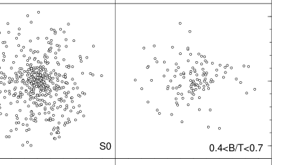
Figure 3: Spatial distribution of galaxies in the ensemble clusters. The projected radii of each galaxy is normalized to the $r_{200}$ of the cluster it belongs to. Left, ec-nearby: projected positions of galaxies in 12 rich nearby clusters. The positions are presented in $r_{200}$ units, and they are separated as elliptical, lenticular and spiral galaxies following the classical Hubble sequence morphological classification. Right, ec-cnoc: projected positions of galaxies in 9 intermediate-redshifts clusters, the galaxies were separated following the B/T criteria (see section 3.1).

We combine the two samples of clusters, in normalized co-ordinates to construct two ensemble working samples, called ec-nearby and ec-cnoc. Figure 3 presents the projected positions of the galaxies inside the r₂₀₀ radius of the ec-nearby and ec-cnoc clusters. To combine the clusters we adopt the same procedure of Carlberg, Yee & Ellingson (1997) and Ramírez & de Souza (1998). The brightest cluster galaxies were used as the nominal centers of each cluster on the sky for the CNOC1 clusters. The galaxy velocities were normalized to the velocity dispersion about the cluster mean, and the projected radii were normalized to the empirically determined r₂₀₀ (see section 3). This procedure diminishes substructure and asphericity to a level where the galaxies can be treated as if they were in a spherical distribution, preserving the radial dependence of the kinematical properties of the samples, and clearing off the effects due to eventually existing local substructures. Before any comparison between both ensembles, it is important to clarify how the different morphological populations will be referred. Due to the selection of only elliptical, lenticular and spiral galaxies in the nearby sample, hereafter the definition of early-type (late-type) galaxy will mean: elliptical (spiral) galaxy in the nearby sample and bulge-dominated (disk-dominated) galaxy at intermediate-redshift. Then, the early-type galaxies not include the lenticular galaxies in the nearby sample, nor the intermediate B/T class galaxies at intermediate-redshift. Also, we must to note that the late-type definition in the nearby clusters excluding the irregular galaxies.

4.1 Projected position distribution

From the Figure 3 we readily noted that the spatial distributions of the late-type galaxies are broader than those for the early-type galaxies, in both samples. This morphological segregation had already been detected in the nearby sample and seems to be also present in the CNOC1 data. A useful quantitative parameter to compare the spatial distribution of each morphological class is the concentration C, listed and defined in Table 1. We found that late-type galaxies tend to present a mean concentration lower than that for early-type galaxies. The typical values for the late-type galaxy populations are: C${}_{S-nearby}=0.40$ and C${}_{S-cnoc}=0.31$. For the more concentrated early-type galaxies the values are C${}_{E-nearby}=0.59$ and C${}_{E-cnoc}=0.42$, and for the intermediate-type it is C${}_{S0-nearby}=0.50$ and C${}_{S0-cnoc}=0.41$. Although it is clear that the concentration parameter is higher for the early-type galaxies in both samples the effect is less pronounced in the case of the intermediate-redshift clusters.

Figure 4 shows the morphology-radius relation that galaxies separated by the B/T criteria follow. This figure shows that the bulge-dominated galaxies are centrally concentrated while the disk-dominated population prefers the periphery. This simply shows the morphology-density (Dressler 1980) or morphology-radius (Whitmore, Gilmore, & Jones 1993) relation over a wide range in cluster-centric distance. The field galaxies included in the CNOC1 survey are also included in the plot.

4.2 Kinematical segregation

Figure 5 presents a summary of several cluster properties as a function of $z/(1+z)$. For low values of redshifts $z/(1+z)\rightarrow z$, and it is proportional to the look-back time ($\tau$) when $\Omega_{0}\rightarrow 0$. In fact, $\tau=z/(1+z)H_{o}^{-1}$ Gyr when $\Omega_{0}=0$. We prefer this variable because the clusters with redshifts lower than 0.1 lay more separated in a plot with this scale than in a linear z scale, which is also labeled in the upper axis.

Figure 5a shows the distribution of the radius r₂₀₀ in $h^{-1}$ Mpc . The dotted and dashed lines represent the r₂₀₀ of the Coma and Virgo clusters, respectively. None of the CNOC1 clusters is as massive as Coma and three of them have significantly low masses. Figures 5b and 5c show the ratio between the velocity dispersion of late- and early-type galaxies, $\sigma_{S}/\sigma_{E}$, and the ratio between intermediate and early-type galaxies, $\sigma_{S0}/\sigma_{E}$, respectively. As can be seen late-type galaxies at low and intermediate-redshifts show similar values, while the intermediate galaxies display values from $\sigma_{S0}/\sigma_{E}\sim 0.50$ to $\sim$1.8 in both samples. It has previously been suggested that late-type galaxies are just now being captured while early-type galaxies may have been in the cluster since the initial formation, representing the relaxed and virialized population, respectively (see references in section 1). Then, a value of $\sqrt{2}$ must be expected (dot-and-dashed line in the Figure 5b and 5c), however in most clusters the ratio is lower. Actually, the mean values are $\sigma_{S}/\sigma_{E}=1.14\pm 0.07$ (bi-weighted dispersion of 0.18) for the nearby sample and $\sigma_{S}/\sigma_{E}=1.17\pm 0.06$ (bi-weighted dispersion of 0.18) for the CNOC1 data. The velocity dispersion of the late-type galaxy population is approximately 15% higher than the velocity dispersion for the early-type galaxies. These results show the existence of a kinematical segregation in both samples — nearby and intermediate-redshift — where the population of early-type galaxies always have a lower velocity dispersion than the population of late-type galaxies. The similar values along the redshift suggest that no-evolution for this type of segregation is present.

Figure 5d shows the distribution of the concentration as a function of redshifts, where the dotted line represents the Coma cluster concentration, and the dashed line correspond to the Virgo cluster concentration, and open diamonds show the concentrations of nine Dressler et al. (1997) (hereafter D97) clusters. D97 measured the concentration of 10 clusters at intermediate-redshifts, using galaxies well inside the central region that cover $\sim$ 0.5-0.8 $h^{-1}$ Mpc (i.e. inside the corresponding $r_{200}$ if they have $\sigma<1200$  km s^-1). They re-evaluated the T-$\Sigma$ relation, using these clusters, finding that the more concentrated clusters are the most affected by the T-$\Sigma$ relation. We observe that most of the nearby clusters have similar concentration values — i.e. concentration around 0.42-0.52 — and they are more concentrated than the intermediate-redshift cluster. The CNOC1 clusters appear with concentrations similar to the low concentration cluster of D97 sample. Then, in agreement with the conclusions of D97 we must expect a lower morphological segregation within the CNOC1 clusters.

4.3 Lenticular galaxies evolution

Finally, in the last two plots of Figure 5 we detected evolution comparing the numbers of late- and intermediate-type to early-type galaxies. In this case we are based in the fact that early-type galaxies must correspond to the oldest population in the cluster — i.e. if they were formed by merging, that must have happened at the beginning of the cluster formation, or if they were formed in a monolithic way they were formed all together not after $z=2$ — and we are also assuming that their numbers kept constant along the cluster life-time. In D97 the ratio of lenticular to elliptical galaxies is cited as an indicator of evolution, and they suggest this ratio decreases with redshift. This is the same tendency found in our samples, as Figure 5f shows. Although, when we compare our data (filled circles in Figure 5f), with those of D97, where a visual morphological classification with HST images was used (open diamonds in Figure 5f), we observe an underestimation of our number of intermediate-type galaxies. This is not only an effect of the difference between morphological classification methods, because the nearby sample — where the classical visual morphology classification was also used — follow the same tendency of the CNOC1 intermediate-redshifts clusters. Nevertheless, in all the cases the number of intermediate-type galaxies is significantly lower at higher redshifts. In fact, the mean value of $N_{S0}/N_{E}$ is $1.46\pm 0.34$ for the nearby sample and $0.43\pm 0.04$ for the CNOC1 sample. Unfortunately, the physical meaning of this evolution is still in discussion and the problem with the misidentification between elliptical and lenticular galaxies is always present. Interesting is to note that when the late-type galaxies are compared with the early-type galaxies the ratio $N_{S}/N_{E}$ (Figure 5e) is almost constant, and they have similar values of that of D97 sample.

5 Segregation detected in the average deviation of the velocity distribution

The average deviation $|u|$ defined in section 2, is useful to connect the line-of-sight velocity distribution of a population with the family of orbits they represent. RdS98 analyzed the behavior of this parameter for a sample of 18 nearby clusters, and concluded that elliptical galaxies have more eccentric orbits than spiral galaxies. In this section we investigate if the results found for the nearby cluster sample also apply for the CNOC1 sample.

The velocity average deviation normalized by the velocity dispersion, $|u|$, was calculated for each population class as follow:

$$|u|=\frac{1}{N}\sum_{i=1}^{N}|v_{i}-v_{cl}|/\sigma_{cl}$$

where N is the number of galaxies of each morphological class, $v_{i}$ is the line-of-sight velocity, $v_{cl}$ and $\sigma_{cl}$ are the mean velocity and velocity dispersion of the cluster, and they were calculated with the bi-weighted estimators (Beers et al 1990). Table 2 presents the average deviation and other kinematical properties of all morphological classes in the nearby and CNOC1 clusters. Column (1) shows the name of the cluster, in the case of Virgo the first entry (Virgo-all) corresponds to the whole cluster, considering as a part of the cluster all the substructures detected by Binggeli, Popescu & Tammann (1993), inside $r_{200}$, the second entry (Virgo-A) corresponds to the main cluster only, part A. The columns (2), (3) and (4) present the following properties for the late-type galaxies: number of galaxies inside the r₂₀₀ radius, velocity dispersion normalized by the cluster velocity dispersion, and average deviation also normalized by the velocity dispersion with their errors to the 68% confidence level. Columns (5), (6) and (7) show the same properties described above for intermediate-type galaxies and columns (8), (9) and (10) for early-type galaxies. When less than 6 galaxies were available the dispersion and the average deviation were not calculated. In Figure 6 we plot the distribution of the average deviation for the late-, intermediate-, and early-type galaxies as a function of the same variable $z/(1+z)$ used in Figure 5. The dotted lines show the expected value of $|u|=0.77$, which represents the highest value bellow which an eccentric orbit can be unambiguously identified, as was described in section 2. For clusters below the dotted we should have that the radial velocity dispersion is larger than the transversal velocity dispersion, $\sigma_{R}>\sigma_{\perp}$, under the assumption of Gaussian velocity field adopted in the present study.

There is a possible bias toward higher values of average deviation due to substructures within clusters, because an artificial enhancement is introduced in the projected velocity distribution. This bias could be more important in the intermediate redshift sample, where substructures are hardly detected. Cen (1997) using n-body simulations suggested that the presence of substructures modifies the velocity distribution in a complex way, but the final velocity dispersion is slightly affected. He estimated variations of the final velocity dispersion of only 5% and 9% within 0.5 and 1.0 $h^{-1}$ Mpc , respectively. Another study is presented in Bird et al. (1996), using observational data, where they noted that the existence of substructures is an important factor to determine the dynamical parameters, but the effect is reduced when the data is restricted to a region inside the virial radius, as we made. It is worthwhile to mention that variations on the velocity dispersion due to substructures could increase or reduce the velocity dispersions (Bird, 1994), a fact which is not consistent with spirals always presenting an slightly larger dispersion than ellipticals. Then, the effect produced by substructures seems to be weak enough to allow the segregation be detected. However, to test how the average deviation could be modified by substructures we applied the method to the Virgo cluster, taking into account the substructures detected by Binggeli, Popescu & Tammann 1993, (BPT93). First we worked with the main body of Virgo, called part A in BPT93, then the same method was applied including the part B and the clouds W and W’. All samples were limited to the region inside the r₂₀₀ radius. The results are presented in the two Virgo’s entry in the Table 2. Both samples show very similar results and differences between spiral, lenticular and elliptical populations are detected on spite of the substructures.

5.1 Late and early-type galaxies

Figure 6 shows the segregation at low redshifts previously detected by RdS98 (see their Figure 4), but now considering galaxies inside r₂₀₀ radius instead of the limiting radius of 1.0 $h^{-1}$ Mpc and 2.5 $h^{-1}$ Mpc adopted in that analysis. The segregation at low redshift shows that elliptical galaxies have $|u|$ values corresponding to highly eccentric orbits, while the spiral galaxies have orbits that are nearly isotropic, circular or slightly radial. Although in general the population of early-type galaxies in the CNOC1 clusters follow the same tendency of those of the nearby clusters, having also lower average deviation values, the clear segregation detected for clusters at $z<0.1$ is not so obvious at higher redshifts. This result could indicate a real evolution of the orbit shapes inside the $r_{200}$ radius, where the early-type population only recently got more eccentric in their orbits, and the population of late-type galaxies kept in circular or isotropic orbits. However, the distribution of average deviations of early-type galaxies in the CNOC1 sample have cases as ms1008-12 with orbits as eccentric as the nearby elliptical galaxies. We must note that the intermediate-type galaxies in the nearby sample follow the same behavior as the early-type population. However, at intermediate redshift the small number of intermediate-type galaxies, producing a behavior not well defined in their kinematical parameters.

To further quantify the degree of significance of the differences between the late-type and early-type galaxies along the redshift, we have applied statistical tests. The main goal is to verify if the observed distributions of the average deviations in Figure 6, could come from the same parent distribution. The same two-sampling tests were applied to all clusters. The tests applied were developed in IRAF/STSDAS (twosampt and kolmov). The results are presented in Table 3, where columns show: (1) the two population being compared, (2) the sample and the morphological criteria, (3) the number of clusters used, and (4) the mean, the error and the dispersion of the average deviation distribution of each sample. The four last columns present the probability, expressed in percentage, of the two compared population belong to the same distribution, using the: (5) K-S Test, (6) Gehan’s Generalized Wilcoxon Test, (7) the Logrank Test and the (8) Peto & Prentice Generalized Wilcoxon Test. The statistical tests show a significant difference between the average deviation distribution of the local spiral and elliptical galaxies at the 99% of confidence level. In the case of bulge- and disk-dominated galaxies at intermediate-redshifts the distributions of the average deviation are different at the 67-89% of confidence level, depending of the statistical test. Then, the difference in the velocity anisotropies seems to exist but is weaker than those for the nearby galaxies.

5.2 Red and blue galaxies

Carlberg et al. (1997) compared the properties of the CNOC1 galaxies separating them by colors. They applied the Jeans equation of stellar hydrodynamical equilibrium to the red and blue subsamples, and they found that both populations give separately statistically identical cluster mass profiles. This is strong evidence that the CNOC1 clusters are effectively systems in equilibrium. Motivated by this work we have also repeated the analysis separating the galaxies by colors. Unfortunately we do not have access to homogeneous data on colors for the nearby clusters. A comparison between nearby and intermediate-redshift clusters requires complete data color for both samples with the same set of filters. Therefore the comparison between red and blue galaxies is applied to the CNOC1 data only.

The criteria to separate the red and blue galaxies was the following: (i) galaxies with (U-V)${}_{0}\leq 1.4$ were defined as blue galaxies, associated to the late-type galaxies, (ii) galaxies with (U-V)${}_{0}>1.4$ were defined as red galaxies, associated to the early-type population. Applying our orbital analysis to these two subsamples we find that the average deviation of both populations, in all clusters, have very different distributions (different at the 99% confidence level). The last line in Table 3 shows this result and Table 4 shows in detail the properties of these populations. In this case we are working with only 7 of the 9 clusters because ms1455+22 and ms0440+02 have less than 6 blue galaxies, and no-statistical results are possible with this number of objects. The mean average deviation of the blue population is $|u|=1.02\pm 0.09$ (dispersion of 0.21) and for the red population is $|u|=0.70\pm 0.02$ (dispersion of 0.06). Therefore, similarly as occurred with nearby ellipticals, the red galaxies observed at intermediate-redshift also have more eccentric orbits than the blue galaxies. In addition, we observe that the mean velocity dispersion of the red and blue galaxy populations — calculated with the velocity dispersion of each population normalized to the velocity dispersions of the respectively cluster — are 0.96 $\pm$ 0.04 and 1.29 $\pm$ 0.09, respectively. That is, the velocity dispersion of blue cluster galaxies is about 30% higher than for red galaxies. This quantity is larger than the difference between elliptical and spiral at low redshift and this one of disk- and bulge-dominated galaxies at intermediate-redshift.

Before any consideration about the notable difference between red and blue galaxy population inside $r_{200}$, we must mention two important characteristic of these subsamples. First, the difference detected here is not in contradiction with the conclusion of Carlberg et al.(1997) about red and blue galaxies in the CNOC1 survey being systems in equilibrium with the gravitational potential of their own clusters. As was explained in RdS98, the global parameters as velocity dispersions are independent of the existence of any difference in the velocity anisotropy. And second, unfortunately up to the limit of $M_{r}^{k}=-18.5$ mag, about 85% of the cluster galaxies inside r₂₀₀ fall into the red subsample. This effect produce a limiting factor in the precise numerical agreement because there are relatively few blue galaxies in clusters, meaning that the mean velocity dispersion and average deviation are less accurately measured than those for red galaxies. On spite of the few galaxies, the behavior of the blue population in all the clusters is always in the same direction (see Table 4). If the blue galaxies are galaxies rich in gas they could represent the star formation activity of the cluster. This activity could be due to an internal perturbation (e.g. early stage of the gas consumption), external perturbations (e.g. tidal effect by near companions or recent merging), or due a mix of these two (e.g. internal response to the galactic harassment). Define how all of these perturbations will affect the observed stellar distribution is a hard task. However, the orbital properties can produce measurable properties compatible with the star formation activity. The objects with very eccentric orbits reach the densest regions of the cluster and are more prompt to suffer perturbations from other galaxies. Although the high relative velocities of the galaxies in the cluster center makes merging unprovable, the accumulated effect of these perturbations could remove the gas content of the galaxies, dimming the star formation rates (e.g. Fujita et al. 1999). In this cases, the blue galaxies in clusters tends to appear redder after some crossing times due to the velocity anisotropy. This could be the case of the A2390 cluster studied by Abraham et al. (1996). In fact, they found that the blue galaxies in this cluster are being altered by the cluster environment, such that some of the their members are likely leaving the blue population to join the red population. Then, if the other clusters in the CNOC1 survey have velocity anisotropy, as A2390 cluster, our finding that red galaxies have more eccentric orbits than blue galaxies is consistent with a modification of the star formation activity by an orbital-segregation.

6 Conclusion

We presented a kinematical analysis of clusters at intermediate-redshifts. They were analyzed looking for the existence of an orbital-segregation, in the sense that galaxies with different morphological types have different orbit families, as was previously found for ellipticals and spirals in nearby clusters. The velocity anisotropies of each morphological population was estimated by the use of the average deviation of the line-of-sight velocity, which is associate to the orbital shapes, assuming a Gaussian distribution having different dispersions along the radial and the transversal directions.

The differences in the average deviation of velocity distributions of elliptical, lenticular and spiral galaxies detected inside the 2.5 $h^{-1}$ Mpc in nearby rich clusters (RdS98) is stronger inside the more interesting in physical meaning $r_{200}$ radius. These differences correspond to different anisotropies and it corresponds to an stronger orbital-segregation. In this case the early-type galaxies, inside the $r_{200}$ radius, have orbits more eccentrics than the late-type galaxies, and the intermediate-type galaxies share an intermediate orbital family.

When the procedure applied to the nearby clusters is applied to a sample of intermediate-redshifts cluster, as the CNOC1 survey, an orbital-segregation is again detected. However, this time the differences is between the bulge-dominated galaxies and the disk-dominated galaxies, and the orbital-segregation is less strong than in the nearby sample. Moreover, when the orbits of the red and blue galaxies of the intermediate-redshift sample are compared the strongest orbital segregation is found. This result suggests the orbital segregation seems to modify more efficiently the star formation activity than the internal shape of the galaxies.

Then, our results impose a further restriction on the plausible models of cluster of galaxies formation. Along the covered redshifts the models must reproduce the observed velocity field anisotropy of each morphological type. In this case the early-type galaxies are evolving very fast from z=0.4 to 0, and late-type galaxies remain with their orbits without obvious evolution. However we cannot discard the possibility that this could be an effect of comparing different population when we associate the elliptical galaxies in nearby clusters to the bulge-dominated galaxies at intermediate-redshifts. Unfortunately, in the case of intermediate-type galaxies, their behavior at higher redshifts is not so clear as in the nearby cluster, and we have — besides the always present problem of misidentification — the problem of the dramatic decrease in number.

Finally, some interesting question are opened: Does the orbital-segregation represent the tendency of early-type galaxies to preserve the initial conditions of an anisotropic collapse? In effect, this type of collapse studied with high resolution n-body simulations and semi-analytical models forms clusters with an anisotropic velocity distribution of their members. These clusters are different from those obtained in a classical spherical collapse, without taking into account the anisotropy in large-scale initial conditions. Cosmological n-body simulations have shown that, in the most scenarios, the matter in filaments collapses into dark matter halos, and these flow along filaments towards the potential minima, where they form galaxy clusters. The collapse is therefore a highly anisotropic process (West, Villumsen & Dekel 1991, Tormen 1997, Tormen, Diaferio & Syer 1998; Ghigna et al. 1998; Dubinski 1998; Splinter et al. 1997). For example, Tormen (1997) studying cluster formation with n-body simulations found that more massive satellites move along slightly more eccentric orbits, which penetrate deeper in the cluster. Also, he found that the shape and orientation of the final cluster and its velocity ellipsoid are strongly correlated with each other and with the infall pattern of merging satellites, suggesting that cluster alignments is related to the anisotropy in the velocity. In addition, the properties of dark matter halos within rich clusters studied by Ghigna et al. (1998) present an orbital distribution close to isotropic, however the circular orbits are rare and the radial orbits are common. Although, the interesting results cited above are more representative of the dark-matter distribution, few has been done to compare with real clusters. Only some observations of distribution of structure in X-ray clusters (West, Jones & Forman 1995) seem indicate that anisotropic collapse is common in also in real clusters. Nevertheless, why only elliptical galaxies are able to preserve the initial conditions? And why the youngest sample shows very eccentric orbits only for red galaxies? Could this be the result of a morphological transformation within an anisotropic collapse? In this case, how the strength of this transformation will depend of the galaxy orbit?. That question, must be studied and clusters are higher redshift must be studied.

Table 1: Cluster kinematic parameters from galaxies inside $r_{200}$

Name	N	$r_{200}$	z	$\sigma_{r_{200}}$		C	Note
		($h^{-1}$ Mpc )		( km s-1)
				——————-
				Value     Error
(1)	(2)	(3)	(4)	(5)		(6)	(7)
CNOC1
ms0016+16	73	1.5	0.5473	1449	124	0.44	a
ms0451-03	59	1.6	0.5384	1461	116	0.37	a
ms1621+26	43	1.0	0.4259	862	86	0.39
ms0302+16	25	0.9	0.4243	769	112	0.49	b
ms1512+36	27	1.0	0.3716	857	124	0.38	b
ms1358+62	128	1.3	0.3274	1046	61	0.43
ms1224+20	27	1.0	0.3256	824	98	0.35	b
ms1008-12	72	1.3	0.3070	1043	107	0.34
ms1006+12	30	1.2	0.2604	907	86	0.40	b
ms1455+22	57	1.5	0.2566	1095	119	0.25
ms1231+15	65	0.9	0.2348	686	59	0.46
a2390	128	1.7	0.2283	1200	69	0.33
ms0451+02	111	1.6	0.2006	1103	81	0.34
ms0440+02	33	1.0	0.1966	698	86	0.29
ms0839+29	79	1.3	0.1931	933	85	0.46
ms0906+11	92	2.8	0.1712	1918	104	0.33	a
Nearby sample
a0754	57	1.3	0.0542	767	82	0.49
a1644	81	1.5	0.0472	905	86	0.37
a3376	61	1.3	0.0464	756	74	0.50
a1631	46	1.1	0.0464	654	72	0.45
a0119	75	1.4	0.0445	840	94	0.48
a0496	74	1.0	0.0327	615	70	0.65
a1656	453	1.7	0.0233	1033	40	0.51
a0194	51	0.8	0.0178	463	54	0.27
a805s	37	0.9	0.0144	511	58	0.48
a1060	92	1.1	0.0122	647	45	0.65
Fornax	50	0.6	0.0048	347	36	0.52
Virgo	322	1.4	0.0045	802	26	0.43

Table 2: Cluster kinematic parameters by populations

	Disk-dominated or S			Intermediate or S0			Bulge-dominated or E
Name	N	$\sigma_{S}/\sigma_{cl}$	$|u|$	N	$\sigma_{S0}/\sigma_{cl}$	$|u|$	N	$\sigma_{E}/\sigma_{cl}$	$|u|$
(1)	(2)	(3)	(4)	(5)	(6)	(7)	(8)	(9)	(10)
CNOC1
ms1621+26	21	1.07	0.70 $\pm$ 0.14	4	-	-	17	0.97	0.80 $\pm$ 0.10
ms1358+62	41	1.06	0.85 $\pm$ 0.10	19	0.91	0.77 $\pm$ 0.11	61	1.03	0.75 $\pm$ 0.08
ms1008-12	29	0.98	0.69 $\pm$ 0.11	12	1.30	0.96 $\pm$ 0.23	25	0.70	0.46 $\pm$ 0.09
ms1455+22	22	1.14	0.80 $\pm$ 0.16	10	0.97	0.68 $\pm$ 0.21	25	0.88	0.59 $\pm$ 0.10
ms1231+15	25	0.96	0.76 $\pm$ 0.11	12	1.31	0.96 $\pm$ 0.22	28	0.90	0.55 $\pm$ 0.11
a2390	49	1.14	0.89 $\pm$ 0.09	22	0.77	0.56 $\pm$ 0.08	47	0.86	0.65 $\pm$ 0.08
ms0451+02	45	1.04	0.78 $\pm$ 0.09	17	0.93	0.56 $\pm$ 0.16	40	0.99	0.72 $\pm$ 0.08
ms0440+02	12	1.04	0.73 $\pm$ 0.20	9	0.51	0.15 $\pm$ 0.06	10	1.14	0.89 $\pm$ 0.23
ms0839+29	38	0.93	0.57 $\pm$ 0.10	13	1.41	1.12 $\pm$ 0.22	24	0.82	0.65 $\pm$ 0.10
Nearby
a0754	18	1.05	0.67 $\pm$ 0.13	18	0.91	0.70 $\pm$ 0.12	21	1.05	0.54 $\pm$ 0.15
a1644	19	1.08	0.72 $\pm$ 0.17	45	0.95	0.61 $\pm$ 0.07	17	1.09	0.65 $\pm$ 0.15
a1631	6	1.03	0.82 $\pm$ 0.25	33	1.04	0.74 $\pm$ 0.10	7	0.76	0.64 $\pm$ 0.24
a3376	19	1.00	0.75 $\pm$ 0.13	31	1.12	0.75 $\pm$ 0.12	11	0.50	0.21 $\pm$ 0.07
a0119	15	1.14	0.94 $\pm$ 0.18	36	0.87	0.53 $\pm$ 0.09	24	1.02	0.56 $\pm$ 0.16
a0496	16	1.05	0.72 $\pm$ 0.17	31	1.16	0.78 $\pm$ 0.14	27	0.72	0.43 $\pm$ 0.09
a1656	188	1.05	0.73 $\pm$ 0.04	110	1.08	0.72 $\pm$ 0.05	155	0.88	0.59 $\pm$ 0.04
a0194	16	1.12	0.75 $\pm$ 0.15	19	0.73	0.53 $\pm$ 0.12	16	1.06	0.73 $\pm$ 0.16
a805s	14	1.18	0.88 $\pm$ 0.20	15	0.85	0.69 $\pm$ 0.11	8	1.01	0.58 $\pm$ 0.26
a1060	30	1.00	0.79 $\pm$ 0.11	49	0.99	0.76 $\pm$ 0.08	13	0.92	0.47 $\pm$ 0.15
Fornax	13	1.16	0.93 $\pm$ 0.17	19	1.01	0.72 $\pm$ 0.13	18	0.88	0.38 $\pm$ 0.16
Virgo-all	196	1.06	0.85 $\pm$ 0.04	74	0.86	0.63 $\pm$ 0.05	52	0.90	0.64 $\pm$ 0.07
Virgo-A	109	1.12	0.88 $\pm$ 0.05	55	0.76	0.56 $\pm$ 0.08	43	0.89	0.63 $\pm$ 0.06

Table 3: Two-sampling test between populations

$Pop_{1}\times Pop_{2}$	sample	Ncls	$|u|_{Pop_{1}}\;\;\times\;\;|u|_{Pop_{2}}$	KS	GGW	L	PPGW
				%	%	%	%
(1)	(2)	(3)	(4)	(5)	(6)	(7)	(8)
S x E	CNOC1a	9	0.76 $\pm$ 0.03 (0.09) $\times$ 0.67 $\pm$ 0.05 (0.14)	33	14	11	15
	Nearbyb	12	0.79 $\pm$ 0.03 (0.10) $\times$ 0.56 $\pm$ 0.04 (0.14)	0.01	0.01	0.00	0.00
S x S0	CNOC1a	9	0.76 $\pm$ 0.03 (0.09) $\times$ 0.74 $\pm$ 0.12 (0.31)	63	77	23	76
	Nearbyb	12	0.79 $\pm$ 0.03 (0.10) $\times$ 0.70 $\pm$ 0.03 (0.09)	10	1	1	1
E x S0	CNOC1a	9	0.67 $\pm$ 0.05 (0.14) $\times$ 0.74 $\pm$ 0.12 (0.31)	63	50	96	50
	Nearbyb	12	0.56 $\pm$ 0.04 (0.14) $\times$ 0.70 $\pm$ 0.03 (0.09)	3	1	1	1
Blue x Red	CNOC1c	7	1.02 $\pm$ 0.09(0.21) $\times$ 0.70 $\pm$ 0.02 (0.06)	1	0.1	0.01	0.04

Table 4: Cluster kinematic parameters by populations

	Blue-(U-V)${}_{0}\leq 1.4$			Red-(U-V)${}_{0}>1.4$
Name	N	$\sigma_{blue}/\sigma_{cl}$	$|u|$	N	$\sigma_{red}/\sigma_{cl}$	$|u|$
(1)	(2)	(3)	(4)	(5)	(6)	(7)
ms1621+26	7	0.94	0.87 $\pm$ 0.18	36	1.05	0.78 $\pm$ 0.10
ms1358+62	13	1.42	1.20 $\pm$ 0.17	115	0.95	0.70 $\pm$ 0.05
ms1008-12	12	1.55	1.24 $\pm$ 0.27	60	0.86	0.56 $\pm$ 0.07
ms1455+22	5	-	-	52	0.94	0.63 $\pm$ 0.08
ms1231+15	6	0.47	0.76 $\pm$ 0.28	59	1.00	0.73 $\pm$ 0.08
a2390	21	1.16	0.94 $\pm$ 0.13	107	0.97	0.72 $\pm$ 0.05
ms0451+02	25	1.20	0.89 $\pm$ 0.13	86	0.95	0.68 $\pm$ 0.06
ms0440+02	0	-	-	33	1.00	0.73 $\pm$ 0.11
ms0839+29	7	1.50	1.25 $\pm$ 0.41	72	0.93	0.65 $\pm$ 0.07

Figure 1: Average deviation as a function of the anisotropic parameter $\eta$. When the system have isotropic orbits ($\eta=1$) the $|u|$ tends to the value 0.80. Systems with purely radial ($\eta>>1$) or circular orbits ($\eta\rightarrow 0$) have $|u|$ converging to 0.69 and 0.77, respectively.

Figure 2: Color distribution (U-V)₀ of the CNOC1 data when separated by the B/T criteria.

Figure 4: Morphology-radius relation of CNOC1 data. Galaxies were separated as bulge-dominant (B/T $>$ 0.7: fill circles), disk-dominant (B/T $<$ 0.4; open squares), and intermediate galaxies (0.4 $>$ B/T $>$ 0.7; dots). The galaxies at $R/R_{200}>2$ are field galaxies.

Figure 5: Distribution along the variable $z/(1+z)$ of: (a) the radius $r_{200}$ in $h^{-1}$ Mpc , (b) the ratio between velocity dispersion of late- and early-type galaxies, $\sigma_{S}/\sigma_{E}$, (c) the ratio between velocity dispersion of intermediate and early-type galaxies, $\sigma_{S0}/\sigma_{E}$, (d) the concentration of the cluster C inside of $r_{200}$, (e) the ratio between the number of late- and early-type galaxies, $N_{S}/N_{E}$, and (f) the ratio between the number of intermediate- and early-type galaxies, $N_{S0}/N_{E}$. The upper axis, with small numbers, is labeled in redshift scale. The dotted and dashed lines in plots (a) and (d) correspond to the Coma and Virgo clusters, respectively. The dot-and-dashed lines in plots (b) and (c) are the expected ratio of a falling over a virialized system, $\sigma_{fall}/\sigma_{vir}=\sqrt{2}$. The open diamonds correspond to clusters of the Dressler et al. (1997) sample.

Figure 6: Distribution of the velocity average deviation defined as $|u|=<|v_{i}-v_{cl}|/\sigma_{cl}>$, where $v_{cl}$ and $\sigma_{cl}$ are the mean velocity and velocity dispersion of the cluster calculated with the bi-weighted estimator (Beers et al 1990). It is plotted as a function of z/(1+z), which is proportional to the look-back time in a universe with $\Omega_{o}$ = 0. The upper axis, with small numbers, is labeled in redshift scale. The members were separated as late-type(upper plot), intermediate-type (middle plot), or early-type (lower-plot) galaxies. Late-type galaxies, in the clusters at intermediate-redshift are represented by galaxies with the ratio of bulge to disk luminosity of B/T$\leq$0.4, intermediate-type galaxies by 0.4 $<$ B/T $<$ 0.7, and early-type galaxies by B/T$\geq$0.7. The dotted line represents the separation between eccentric orbits ($|u|<0.77$) and approximately circular or isotropic orbits ($|u|\geq 0.77$). As explained in section 2, the value $|u|=0.77$ represents the highest value below which an eccentric orbit can be unambiguously identified.

References

- Abraham et al. (1996) Abraham, R. G., Smecker-Hane, T. A., Hutchings, J. B., Carlberg, R. G., Yee, H. K. C., Ellingson, E., Morris, S., Oke, J. B., & Davidge, T. 1996, ApJ, 471, 694
- Andreon (1994) Andreon, S. 1994, A&A, 284, 801
- Andreon (1996) Andreon, S. 1996, A&A, 314, 763
- Andreon & Davoust (1997) Andreon, S., & Davoust, E. 1997, A&A, 319, 747
- Beers et al. (1990) Beers, T.C., Flynn, K., & Gebhardt, K. 1990, AJ, 100, 32
- Binggeli, Popescu & Tammann (1993) Binggeli, B., Popescu, C.C., & Tammann, G.A. 1993, A&AS, 98, 275
- Binney & Mamon (1982) Binney, J., & Mamon, G.A. 1982, MNRAS, 200, 361
- Binney, Davies & Illingworth (1990) Binney, J., Davies, R., & Illingworth, G. 1990, ApJ, 361, 78
- Bird et al. (1994) Bird, C.M., Davis, D.S., & Beers, T.C. 1994, AJ, 109, 920
- Biviano et al. (1992) Biviano, A., Girardi, M., Giuricin, G., Mardirossian, F., & Mezetti, M. 1992, ApJ, 396, 35
- Biviano et al. (1997) Biviano, A., Katgert, P., Mazure, A., Moles, M., den Hartog, R., Perea, J., & Focardi, P. 1997, A&A, 321, 84
- Butcher & Oemler (1978) Butcher, H., & Oemler, A.Jr. 1978, ApJ, 219, 18
- Carlberg et al. (1996) Carlberg, R. G., Yee, H. K. C., Ellingson, E., Abraham, R., Gravel, P., Morris, S.M., & Pritchet, C.J. 1996, ApJ, 462, 32
- Carlberg Yee & Ellingson (1997) Carlberg, R.G., Yee, H.K.C., & Ellingson, E. 1997, ApJ, 478, 462
- Carlberg et al. (1997) Carlberg, R.G., Yee, H.K.C., Ellingson, E., Morris, S.M, Abraham, R., Gravel, P., Pritchet, C.J., Smecker-Hane, T., Hartwick, F.D.A., Hesser, J.E., Hutchings, J.B., & Oke, J.B. 1997, ApJ, 476, L7
- Cen (1997) Cen, R. 1997, ApJ, 485, 39
- Colless and Dunn (1996) Colless, M., Dunn, A.M. 1996, ApJ, 458, 435
- Dejonghe (1987) Dejonghe, H. 1987, MNRAS, 224, 13
- Dressler (1980) Dressler, A. 1980, ApJ, 236, 351
- Dressler & Shectman (1988) Dressler, A., & Shectman, S.A. 1988, AJ, 95, 985
- Dressler et al. (1997) Dressler, A., Oemler, A.Jr, Couch, W.J., Smail, I., Ellis, R.S., Barger, A., Butcher, H., Poggianti, B.M., & Sharples, R.M. 1998, ApJ, 490, 577
- Dubinski (1998) Dubinski, J. 1998, ApJ, 502, 141
- Fadda et al. (1996) Fadda, D., Girardi, M., Giuricin, G., Mardirossian, F., & Mezetti, M. 1996, ApJ, 473, 670
- Fusco-Fermiano & Menci (1998) Fusco-Fermiano, R., & Menci, N., 1998, ApJ, 498, 95
- Fujita et al. (1999) Fujita, Y., Takizawa, M., Nagashima, M., Enoki, M. 1999, astroph/9904386
- Gerhard (1991) Gerhard, O.E. 1991, MNRAS, 250, 812
- Gerhard (1993) Gerhard, O.E. 1993, MNRAS, 265, 213
- Ghigna et al. (1998) Ghigna, S., Moore, B., Governato, F., Lake, G., Quinn, T., & Stadel, J. 1998, MNRAS, 300, 146
- Girardi et al. (1996) Girardi, M., Fadda, D., Giuricin, G., Mardirossian, F., & Mezetti M. 1996, ApJ457, 61
- Huchra (1985) Huchra, J.P. 1985, in The Virgo Cluster, ESO Workshop Proceedings No 20, eds. Richter O.-G., Binggeli B., (Munich: ESO), p. 181
- Kashikawa et al. (1998) Kashikawa, N., Sekigushi, M., Doi, M., Komiyama, Y., Okamura, S., Shimasaku, K., Yagi, M., & Yasuda, N. 1998, ApJ, 500, 750
- Kendall, Stuart and Ord, (1987) Kendall, M., Stuart, A., Ord, J.K. 1987 in Kendall’s Advanced Theory of Statistics, fifth edition of Volume 1: Distribution Theory, p.52 (Charles Griffin & Co.Ltd., London).
- Merritt (1987) Merritt, D. 1987, ApJ, 313, 121
- Merritt (1996) Merritt, D. 1996, AJ, 112, 1085
- Moss & Dickens (1977) Moss, C., & Dickens, R.J. 1977, MNRAS, 178, 701
- Qian et al. (1995) Qian, E.E., de Zeeuw, P.T., van der Marel, R.P., & Hunter, C. 1995, MNRAS, 274, 602
- Ramírez & de Souza (1998) Ramírez, A.C., & de Souza, R.E. 1998, ApJ, 496, 693
- Sanromà & Salvador-Solé (1990) Sanromà, M., & Salvador-Solé, E. 1990, ApJ, 360, 16
- Schade et al. (1996) Schade, D., Lilly, S.J., Le Fèvre, O., Hammer, F., & Crampton, D., 1996, ApJ, 464, 79
- Scodeggio et al. (1995) Scodeggio, M., Solanes, J.M., Giovanelli, R., & Haynes, M. 1995, ApJ, 444, 41
- Sodré et al. (1989) Sodré, L., Capelato, H., & Steiner, J. 1989, AJ, 97, 1279
- Splinter et al. (1997) Splinter, R.J., Mellot, A.L., Linn, A.M., Buck, C., & Tinker, J. 1997, ApJ, 479, 632
- The & White (1986) The, L.S., & White, S.D.M. 1986, AJ, 92, 1248
- Tormen (1997) Tormen, G. 1997, MNRAS, 290, 411
- Tormen et al. (1998) Tormen, G., Diaferio, A., & Syer, D. 1998, MNRAS299, 728
- Tully and Shaya (1984) Tully, R.B., & Shaya, E.J. 1984, ApJ, 281, 31
- West, Jones & Forman (1995) West, M.J., Jones, C., & Forman, W. 1995, ApJ, 451, L5
- West, Villumsen & Dekel (1991) West, M.J., Villumsen, J.V., & Dekel, A. 1991, ApJ, 369, 287
- Whitmore & Gilmore (1991) Whitmore, B.C., & Gilmore, D.M. 1991, ApJ, 367, 64
- Whitmore, Gilmore, & Jones (1993) Whitmore, B.C., Gilmore, D.M., & Jones, C. 1993, ApJ, 407, 489