The power spectrum of the CfA/SSRS UZC galaxy redshift survey

Abstract

The combined CfA2/SSRS redshift catalog has recently been improved and made public. We compute the redshift-space power spectrum of this catalog using the regions at $-2.5^{\circ}\leq\delta_{1950}\leq 50^{\circ}$ north ($8^{h}\leq\alpha_{1950}\leq 17^{h}$) and south ($20^{h}\leq\alpha_{1950}\leq 3^{h}$, $b\leq-13^{\circ}$) of the Galactic plane, where it is 98% complete down to Zwicky magnitude 15.5 and contains 13,681 galaxies. Our analysis uses Heavens-Taylor mode expansion, Karhunen-Loève data compression and the Fisher matrix technique to compute quadratic band power estimates. This allows an exact calculation of window functions, including the integral constraint, in addition to the production of a power spectrum with uncorrelated error bars. Our results with this larger data set agree well with previous studies. We analyze $101h^{-1}{\rm Mpc}$ and $130h^{-1}{\rm Mpc}$ volume-limited subsets in addition to the full magnitude-limited sample, and our results are well fit by, e.g., $\Lambda$CDM models with bias $b=$1.2, 1.4 and 1.4, respectively. We estimate the effect of extinction using the Schlegel, Finkbeiner & Davis dust map. Our results are exclusively for the redshift space galaxy power spectrum, so they can only be compared with theoretical predictions if appropriate corrections are made for biasing and redshift space distortions.

1. Introduction

The three-dimensional maps of the Universe provided by galaxy redshift surveys provide valuable information about many fundamental cosmological parameters. This has motivated the creation of large data sets such as the Harvard-Smithsonian Center for Astrophysics (CfA), Las Campanas (LCRS) and IRAS 0.6 Jy (PSCz) redshift catalogs, each well in excess of $10^{4}$ galaxies. Even more ambitious projects are currently under way, with the AAT two degree field survey (2dF) aiming for 250,000 galaxies and the Sloan Digital Sky Survey (SDSS) for 1 million. Combining such surveys with measurements from upcoming CMB experiments,e.g., the MAP satellite, enables many cosmological parameters to be measured much more accurately than would be possible using CMB information alone (Eisenstein et al. 1999) — in principle. Achieving this in practice requires that the matter power spectrum $P(k)$ can be accurately measured despite all the complications that are inevitably present in real-world redshift surveys.

This challenge has stimulated a large body of work over the last few years aimed at tackling such real-world issues, ranging from improved models of bias and extinction to the development of powerful new methods for measuring the power spectrum from surveys with arbitrary geometry and selection functions.

The new CfA/SSRS UZC catalog has recently been completed (Falco et al. 1999), made public and had its correlation function (Girardi et al. 2000) and topology (Schmalzing & Diaferio 2000) measured. Since the power spectrum analyses of the original CfA2 and SSRS surveys were performed some time ago (Park et al. 1994; da Costa et al. 1994; Marzke et al. 1994), it is therefore quite timely to apply some of these new methods to this extensive and further improved data set. This is the purpose of the present work. We limit our analysis to the galaxy redshift space power spectrum on large scales, and therefore do not include the important complications of biasing, redshift space distortions or nonlinearities.

The rest of this paper is organized as follows. After describing the UZC data set in Section 2, we present our analysis method in Section 3. The results are given in Section 4, which also tests their robustness to various underlying assumptions. We summarize the conclusions and remaining challenges in Section 5.

2. Data

The previous CfA redshift surveys (Huchra, Vogeley & Geller 1999; Huchra, Geller & Corwin 1995; Huchra et al. 1990; Geller & Huchra 1989; Huchra et al. 1983; Davis et al. 1982) have all been based on the Zwicky catalog of galaxies with magnitude $m_{Zw}\leq 15.5$, involving a heterogeneous sets of galaxy coordinates and redshifts. Falco et al. (1999) recently completed and made public the Updated Zwicky Catalog (UZC), which was improved over its predecessors in a number of ways:

1. Over 5,000 redshifts have been re-measured or uniformly re-reduced.

2. The accuracy of the galaxy coordinates has been improved to better than two arcseconds using the digitized POSS plates.

3. The redshift “blunder rate” has been estimated and substantially reduced.

The sample described in Falco et al. (1999) consists of 19285 galaxies, some without measured redshifts. The sample has subsequently been further improved and extended to 19415 galaxies, available online.

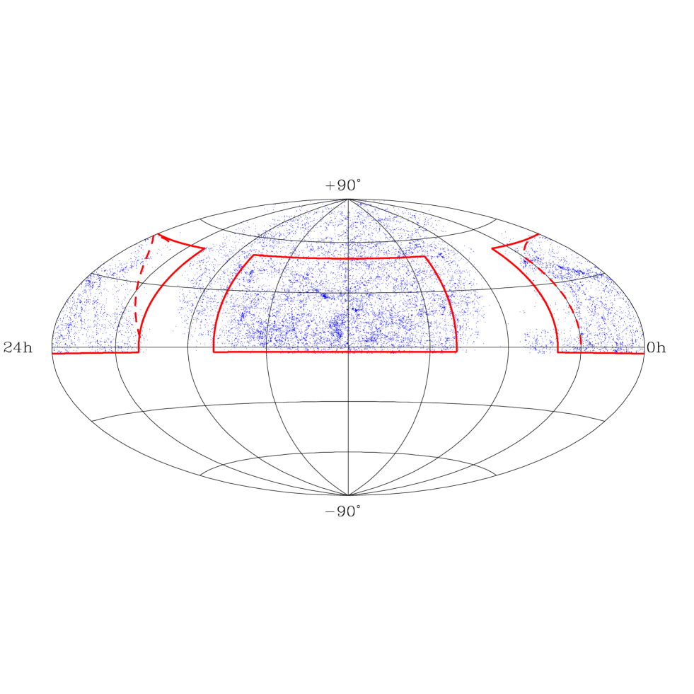
Figure 1.— The 19415 UZC galaxies are shown in Aitoff projection in equatorial coordinates. The two 98% complete subsets are delimited by heavy lines, with the North Galactic subset in the center. We make additional cuts at $b=-13^{\circ}$ and $\alpha=3^{h}$ (dashed lines) to reduce extinction problems.

We use the latest (as of November 1999) version of this data set, which consists of 18,763 galaxies with redshifts. Their angular distribution is shown in Figure 1. Our analysis is limited to the subset defined by $20^{h}\leq\alpha_{1950}\leq 4^{h}$ (hereafter “South”) and $8^{h}\leq\alpha_{1950}\leq 17^{h}$ (hereafter “North”), $-2.5^{\circ}\leq\delta_{1950}\leq 50^{\circ}$, where the sample is 98% complete down to Zwicky magnitude 15.5 (Falco et al. 1999). We also apply a Galactic cut $|b_{II}|>13^{\circ}$ and discard the southern Galactic region with $\alpha_{1950}>3^{h}$ to reduce extinction problems. This leaves a subset consisting of 13,681 galaxies in a region subtending about a quarter of the sky ($10369$ square degrees $\approx 3.16$ steradians). The redshift distribution of these galaxies is shown in Figure 2. Here and throughout this paper, we neglect the cosmic deceleration correction and define the distance to a galaxy in redshift space as simply

$$r\equiv{cz\over H}=(3000h^{-1}\,{\rm Mpc})\>z,$$ (1)

since $z\ll 1$, where $z$ is the galaxy redshift in the CMB rest frame. Figure 2 also shows the radial selection function that we use in our analysis, taken from de Lapparent et al. 1989. It assumes a Schecter luminosity function with parameters $M_{*}=-19.3+5\log h$ and $\alpha=-1.1$. We truncate this magnitude limit radially so that $10^{-3}h^{-1}{\rm Mpc}<r<150h^{-1}{\rm Mpc}$, which leaves 13,184 galaxies. The lower limit removes 32 galaxies with negative redshifts. To facilitate comparison with prior work, we also analyze two volume-limited subsamples of the data, where we keep only galaxies whose absolute magnitude is bright enough that they would have been visible above the $m_{Zw}\leq 15.5$ cut even if they were at the edge of the volume. Following Park et al. 1994, we take these to have depth $101\>h^{-1}\,{\rm Mpc}$ and $130\>h^{-1}\,{\rm Mpc}$, which gives samples of size 2061 and 909, respectively, with a selection function that should in principle be constant within the volume.

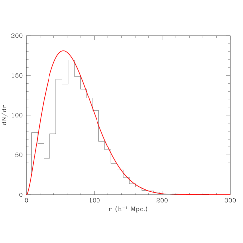
Figure 2.— The redshift distribution of the 98% complete sample of 13,681 galaxies. The smooth curve is the selection function of de Lapparent et al 1989.

3. Method

We analyze the data using the methods described in Tegmark et al. (1998, hereafter “T98”). The analysis consists of the following four steps:

1. Heavens-Taylor pixelization

2. Karhunen-Loève compression

3. Quadratic band-power estimation

4. Fisher decorrelation

We will now describe these steps in more detail.

3.1. Step 1: Heavens-Taylor pixelization

Our raw data consists of $N_{\rm gal}$ three-dimensional vectors ${\bf r}_{\alpha}$, $\alpha=1,...,N_{\rm gal}$, giving the measured positions of each galaxy in redshift space. As discussed in T98, it is convenient to define the overdensity in ${N_{x}}$ “pixels” $x_{i}$, $i=1,...,{N_{x}}$ by

$$x_{i}\equiv\int\left[{n({\bf r})\over{\bar{n}}({\bf r})}-1\right]\psi_{i}({\bf r})d^{3}r=\int{n({\bf r})\over{\bar{n}}({\bf r})}\psi_{i}({\bf r})d^{3}r-m_{i}$$ (2)

for some set of functions $\psi_{i}$ and work with the ${N_{x}}$-dimensional data vector ${\bf x}$ instead of the the $3\times N_{\rm gal}$ numbers ${\bf r}_{\alpha}$. Since the mean density term

$$m_{i}\equiv\int\psi_{i}({\bf r})d^{3}r$$ (3)

has been subtracted out, we have

$$\langle{\bf x}\rangle = {\bf 0},$$ (4)

$$\langle{\bf x}{\bf x}^{\dagger}\rangle = {\bf C}\equiv{\bf N}+{\bf S},$$ (5)

where the shot noise covariance matrix given by

$${\bf N}_{ij}=\int{\psi_{i}({\bf r})\psi_{j}({\bf r})\over{\bar{n}}({\bf r})}d^{3}r$$ (6)

and the signal covariance matrix is

$${\bf S}_{ij}=\int\widehat{\psi}_{i}({\bf k})\widehat{\psi}_{j}({\bf k})^{*}P(k){d^{3}k\over(2\pi)^{3}}.$$ (7)

Here hats denote Fourier transforms and ${\bar{n}}$ is the three-dimensional selection function of the galaxy survey, i.e., ${\bar{n}}({\bf r})dV$ is the expected (not the observed) number of galaxies in a volume $dV$ about ${\bf r}$.

We follow Heavens & Taylor (1995, hereafter “HT”) in choosing our functions $\psi_{i}$ to be spherical waves

$$\psi_{i}({\bf r})=w_{i}(r)Y_{\ell m}(\widehat{\bf r})j_{\ell}(k_{\ell n}r),$$ (8)

where $Y_{\ell m}$ is a spherical harmonic and $j_{\ell}$ a spherical Bessel function. This choice of functions has the advantage (Fisher, Scharf, & Lahav 1994; HT) of forming an almost complete set, separating large and small scales fairly well and allowing efficient computation of $\bf m$ and ${\bf C}$. The pixelized data vector ${\bf x}$ is shown in Figure 3 for one of the volume-limited subsamples.

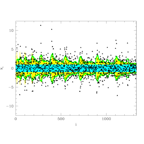
Figure 3.— The triangles show the 1331 elements $x_{i}$ of the data vector ${\bf x}$ (the HT expansion coefficients) for the $130\>h^{-1}{\rm Mpc}$ volume-limited sample. If there were no clustering in the survey, merely shot noise, they would have unit variance, and about $68\%$ of them would be expected to lie within the blue/dark grey band. If our $\Lambda$CDM prior power spectrum were correct, then the standard deviation would be larger, as indicated by the shaded yellow/light grey band. The green/grey curve is the rms of the data points $x_{i}$, averaged in bands of width 25, and is seen to agree fairly well with the shaded band.

Here and throughout, we use a single index $i$ to refer to the triplet $(\ell mn)$ specifying an HT mode. The wavenumbers $k_{\ell n}$ are chosen as in HT so that the derivative of $j_{\ell}(k_{\ell n}r)$ vanishes at a fixed radius $r=R_{\rm max}$ and $j_{\ell}(k_{\ell n}r)$ has $n$ zeros before that. We choose the weight functions $w_{i}$ to be of the form (Feldman, Kaiser & Peacock 1994)

$$w_{i}(r)\propto{{\bar{n}}(r)\over 1+{\bar{n}}(r)P(k_{\ell n})},$$ (9)

normalized such that the shot noise has unit variance, i.e., ${\bf N}_{ii}=1$. Here $P$ is our prior guess for the power spectrum, which we will discuss in more detail in Section 4.3.1. The results turn out to be rather insensitive to this weight function choice — we will return to this issue in more detail in Section 4.3.3.

We avoid the complex issues described in Tadros et al. (1999) by using real-valued spherical harmonics, which are obtained from the standard spherical harmonics by replacing $e^{im\phi}$ by $\sqrt{2}\sin m\phi$, $1$, $\sqrt{2}\cos m\phi$ for $m<0$, $m=0$, $m>0$ respectively. HT show that apart from redshift-space distortions, the signal covariance matrix is given by ${\bf S}={\bf\Psi}{\bf P}{\bf\Psi}^{t}$, where the diagonal matrix

$${\bf P}_{ii^{\prime}}={\bf P}_{\ell mn,\ell^{\prime}m^{\prime}n^{\prime}}\equiv\delta_{ii^{\prime}}P(k_{\ell n})$$ (10)

contains the effect of the power spectrum and the matrix

$${\bf\Psi}_{ii^{\prime}}\equiv\int w_{\ell n}(r)j_{\ell}(k_{\ell n}r)Y_{\ell m}(\widehat{\bf r})j_{\ell^{\prime}}(k_{\ell^{\prime}n^{\prime}}r)Y_{\ell^{\prime}m^{\prime}}(\widehat{\bf r})d^{3}r$$ (11)

which is $\psi_{i}({\bf r})$ expressed in $(\ell mn)$-space and contains the relevant information about the survey geometry. When computing ${\bf\Psi}$, we use the elegant time-saving trick discovered by HT of expanding the angular part of the selection function in spherical harmonics and replacing the angular integral by a sum over Clebsch-Gordan coefficients.

3.2. Step 2: Karhunen-Loève compression

As can be seen in Figure 3, most of the HT coefficients $x_{i}$ have a fairly low signal-to-noise ratio, i.e., ${\bf S}_{ii}/{\bf N}_{ii}\mathrel{\hbox to0.0pt{\lower 3.0pt\hbox{$\mathchar 536\relax$}\hss}\raise 2.0pt\hbox{$\mathchar 316\relax$}}1$ and they are dominated by shot noise. Moreover, the HT modes form a complete set over the entire sky, so they are overcomplete for our case of the UZC catalog which covers only a fraction of the sky. Both of these facts suggest that data compression may be possible, whereby almost all the cosmological information is retained in a smaller set of modes. Such compression would accelerate the matrix operations described in step 3, where the number of operations required grows as the number of modes cubed.

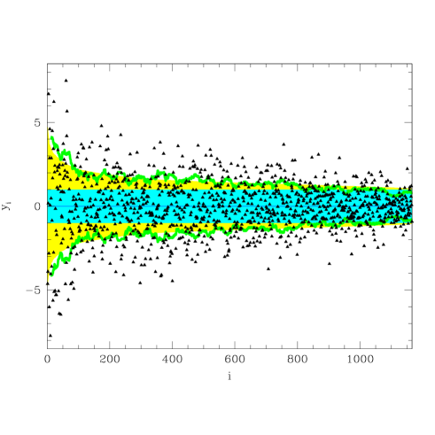
Figure 4.— The triangles show the 1166 elements $y_{i}$ of the compressed data vector ${\bf y}$ (the KL expansion coefficients) for the $130\>h^{-1}{\rm Mpc}$ volume-limited sample. If there were no clustering in the survey, merely shot noise, they would have unit variance, and about $68\%$ of them would be expected to lie within the blue/dark grey band. If our $\Lambda CDM$ prior power spectrum were correct, then the standard deviation would be larger, as indicated by the shaded yellow/light grey band. The green/grey curve is the rms of the data points $x_{i}$, averaged in bands of width 25, and is seen to agree better with the yellow/light grey band than the blue/dark grey band.

We therefore subject the data vector ${\bf x}$ to Karhunen-Loève compression. This method (Karhunen 1947) was first introduced into large-scale structure analysis by Vogeley & Szalay (1996). It was recently applied to the Las Campanas redsift survey (Matsubara et al. 1999) and has been successfully applied to Cosmic Microwave Background data as well, first by Bond (1995) and Bunn (1995). We define a new data vector

$${\bf y}\equiv{\bf B}^{t}{\bf x},$$ (12)

where ${\bf b}$, the columns of the matrix ${\bf B}$, are the ${N_{x}}$ eigenvectors of the generalized eigenvalue problem

$${\bf S}{\bf b}=\lambda{\bf N}{\bf b},$$ (13)

sorted from highest to lowest eigenvalue $\lambda$ and normalized so that ${\bf b}^{\dagger}{\bf N}{\bf b}={\bf I}$. This implies that

$$\langle y_{i}y_{j}\rangle=\delta_{ij}(1+\lambda_{i}),$$ (14)

which means that the transformed data values ${\bf y}$ have the desirable property of being uncorrelated. In the approximation that the distribution function of ${\bf x}$ is a multivariate Gaussian, this also implies that they are statistically independent — then ${\bf y}$ is merely a vector of independent Gaussian random variables. Moreover, equation (13) shows that the eigenvalues $\lambda_{i}$ can be interpreted as a signal-to-noise ratio $S/N$. Since the matrix ${\bf B}$ is invertible, the final data set ${\bf y}$ clearly retains all the information that was present in ${\bf x}$. In summary, the KL transformation partitions the information content of the original data set ${\bf x}$ into ${N_{x}}$ chunks that are

1. mutually exclusive (independent),

2. collectively exhaustive (jointly retaining all the information), and

3. sorted from best to worst in terms of their information content.

Figure 4 shows that most of our KL coefficients $y_{i}$ have a signal-to-noise ratio $\lambda\ll 1$, so that the bulk of the cosmological information is retained in the first ${N_{y}}$ coefficients, ${N_{y}}\ll{N_{x}}$.

In our case, numerical considerations force an additional compression step. The above-mentioned overcompleteness means that certain linear combinations of modes vanish almost completely within the angular mask of the survey (shown in Figure 1). This makes many of of the eigenvalues of ${\bf S}$ and ${\bf N}$ essentially zero and poses a numerical problem when solving equation (13), since the standard reduction to an ordinary eigenvalue problem by Cholesky decomposing ${\bf N}$ or ${\bf S}$ fails when both are singular. Adding a small number to the diagonal elements of ${\bf N}$ also fails to solve the problem: since these redundant modes are tiny, avoiding to vanish completely mostly because of rounding errors, they have a minute contribution from both signal and noise and therefore will not automatically get weeded out by a cut on the signal-to-noise $\lambda$. We therefore begin our compression by expanding the data in the eigenvectors of ${\bf S}$ and get rid of these redundant junk modes by throwing away all eigenmodes with eigenvalues below $10^{-6}$. We then subject the new compressed data set to KL compression.

In conclusion, this step takes the vector ${\bf x}$ and its covariance matrix ${\bf C}$ from Figure 3 and compresses it into the smaller vector ${\bf B}^{t}{\bf x}$ and its covariance matrix ${\bf B}^{t}{\bf C}{\bf B}$, illustrated in Figure 4.

3.3. Step 3: Quadratic band-power estimation

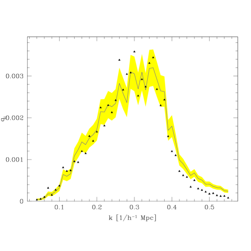
Figure 5.— The triangles show the 52 elements $q_{i}$ of the raw quadratic band-power estimators ${\bf q}$ for the $130\>h^{-1}{\rm Mpc}$ volume-limited sample. If the fiducial $\Lambda$CDM power spectrum were correct, then about $68\%$ of them would be expected to lie within the shaded yellow/light grey band, centered on the solid curve.

In this step, we perform a much more radical data compression by taking certain quadratic combinations of the data vector that can easily be converted into power spectrum measurements.

We parametrize the power spectrum as a piecewise constant function with ${N_{p}}$ “steps” of height $p_{i}$, which we term the band powers and group into an ${N_{p}}$-dimensional vector ${\bf p}$. Thus $P(k)=p_{i}\ {\rm for}\ k_{i-1}\leq k<k_{i}$, where

$$0=k_{0}<k_{1}<...<k_{N_{p}}.$$ (15)

We use ${N_{p}}=52$ bands, most of them with bandwidth $\Delta k=0.01/h^{-1}\>{\rm Mpc}$, which should provide fine enough $k$-resolution to resolve any baryonic wiggles and other spectral features that may be present in the power spectrum. This means that we can write

$${\bf C}=\sum_{i=0}^{{N_{p}}}p_{i}{\bf C},{{}_{i}}$$ (16)

where the derivative matrix ${\bf C},{{}_{i}}\equiv\partial{\bf C}/\partial p_{i}$ is the contribution from the $i^{th}$ band and is computed by simply limiting the implicit sums in the matrix multiplication ${\bf S}={\bf\Psi}{\bf P}{\bf\Psi}^{t}$ to those lines and columns of the power spectrum matrix ${\bf P}$ where $k_{\ell n}$ lies in the $i^{th}$ band; $k_{i-1}<k_{\ell n}<k_{i}$. For notational convenience, we included the noise term in equation (16) by defining ${\bf C},{{}_{0}}\equiv{\bf N}$, corresponding to an extra dummy parameter $p_{0}=1$ giving the shot noise normalization.

Our quadratic band power estimates are defined by

$$q_{i}\equiv{1\over 2}{\bf x}^{t}{\bf C}^{-1}{\bf C}_{,i}{\bf C}^{-1}{\bf x},$$ (17)

$i=1,...,{N_{p}}$. These numbers are shown in Figure 5, and we will group them together in an ${N_{p}}$-dimensional vector ${\bf q}$. Note that whereas ${\bf x}$ and ${\bf y}$ (and therefore ${\bf C}$ and ${\bf B}$) were dimensionless, ${\bf p}$ has units of power, i.e., volume. Equation (17) therefore shows that ${\bf q}$ has units of inverse power, i.e., inverse volume. It is not immediately obvious that the vector ${\bf q}$ is a useful quantity. It is certainly not the final result (the power spectrum estimates) that we want, since it does not even have the right units. Rather, like ${\bf y}$, it is a useful intermediate step. In the approximation that the pixelized data has a Gaussian probability distribution (a good approximation in our case because of the central limit theorem, since $N_{\rm gal}$ is large) ${\bf q}$ has been shown to retain all the information about the power spectrum from the original data set (Tegmark 1997, hereafter “T97”). The numbers $q_{i}$ have the additional advantage (as compared with, e.g., maximum-likelihood estimators) that their properties are easy to compute: their mean and covariance are given by

$$\langle{\bf q}\rangle = {\bf F}{\bf p},$$ (18)

$$\langle{\bf q}{\bf q}^{t}\rangle-\langle{\bf q}\rangle\langle{\bf q}\rangle^{t} = {\bf F},$$ (19)

where ${\bf F}$ is the Fisher information matrix (Tegmark et al. 1997)

$${\bf F}_{ij}={1\over 2}\hbox{tr}\,\left[{\bf C}^{-1}{\bf C}_{,i}{\bf C}^{-1}{\bf C}_{,j}\right].$$ (20)

Quadratic estimators were first derived for galaxy survey applications (Hamilton 1997ab). They were accelerated and first applied to CMB analysis (T97; Bond, Jaffe & Knox 2000).

In conclusion, this step takes the vector ${\bf y}$ and its covariance matrix ${\bf B}^{t}{\bf C}{\bf B}$ from Figure 4 and compresses it into the smaller vector ${\bf q}$ and its covariance matrix ${\bf F}$, illustrated in Figure 5. Although equation (18) shows that we can obtain unbiased estimates of the true powers ${\bf p}$ by computing ${\bf F}^{-1}{\bf q}$, there are even better options, as will be described in the next subsection.

3.4. Step 4: Fisher decorrelation

Let us first eliminate the shot-noise dummy parameter $p_{0}$, since we know its value. We define ${\bf f}$ to be the $0^{th}$ column of the Fisher matrix defined above ($f_{i}\equiv{\bf F}_{i0}$) and restrict the indices $i$ and $j$ to run from $1$ to ${N_{p}}$ from now on, so ${\bf f}$, ${\bf q}$ and ${\bf p}$ are ${N_{p}}$-dimensional vectors and ${\bf F}$ is an ${N_{p}}\times{N_{p}}$ matrix. Since $p_{0}=1$, equation (18) then becomes $\langle{\bf q}\rangle={\bf F}{\bf p}+{\bf f}$.

We now define a vector of shot noise corrected band power estimates

$$\widehat{\bf p}\equiv{\bf M}({\bf q}-{\bf f}),$$ (21)

where ${\bf M}$ is some matrix whose rows are normalized so that the rows of ${\bf M}{\bf F}$ sum to unity. Using equations (18) and (19), this gives

$$\langle\widehat{\bf p}\rangle = {\bf W}{\bf p},$$ (22)

$$\langle\widehat{\bf p}\widehat{\bf p}^{t}\rangle-\langle\widehat{\bf p}\rangle\langle\widehat{\bf p}\rangle^{t} = {\bf M}{\bf F}{\bf M}^{t},$$ (23)

where ${\bf W}\equiv{\bf M}{\bf F}$. We will refer to the rows of ${\bf W}$ as window functions, since they sum to unity and equation (22) shows that $\widehat{p}_{i}$ probes a weighted average of the true band powers $p_{j}$, the $i^{th}$ row of ${\bf W}$ giving the weights.

3.4.1 The minimum-variance choice

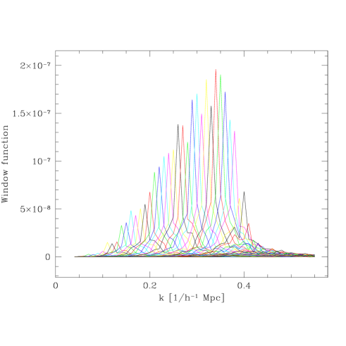
Figure 6.— The rows of the Fisher matrix are shown for the $130\>h^{-1}{\rm Mpc}$ volume-limited sample. The $i^{th}$ row typically peaks at the $i^{th}$ band, the scale $k$ that the band power estimator $q_{i}$ was designed to probe. Large amplitudes signify large information — if all curves had exactly the same shape, then the area under the $i^{th}$ curve would be $(\Delta{\bf p}_{i})^{-2}$, the inverse variance of $q_{i}$ when normalized as a band power estimator. The turnover in the envelope at $k\sim 0.3/h^{-1}{\rm Mpc}$ reflects our omission of HT modes probing smaller scales.

What is the best choice of the matrix ${\bf M}$? A simple and natural choice is

$${\bf M}_{ij}=\left(\sum_{j=1}^{{N_{p}}}{\bf F}_{ij}\right)^{-1}\delta_{ij},$$ (24)

i.e., ${\bf M}$ diagonal (T97; Bond, Jaffe & Knox 2000). Figure 6 plots the rows of the Fisher matrix, which have the same shape as the window functions for this choice of ${\bf M}$. As is seen in this figure, all elements of ${\bf F}$ are positive. This is guaranteed by the fact that the matrices in equation (20) are all positive definite.

3.4.2 The unbiased choice

Another interesting choice is (T97)

$${\bf M}={\bf F}^{-1},$$ (25)

which gives ${\bf W}={\bf I}$. In other words, all window functions are Kronecker delta functions, and $\widehat{p}$ gives completely unbiased estimates of the band powers, with $\langle\widehat{p}\rangle=p_{i}$ regardless of what values the other band powers take. A drawback of this choice is that the new covariance matrix of equation (23) becomes ${\bf F}^{-1}$, which usually gives substantially larger error bars ($\Delta p_{i}\equiv{\bf M}_{ii}^{1/2}=[({\bf F}^{-1})_{ii}]^{1/2}$) than the first method, anti-correlated between neighboring bands.

3.4.3 The uncorrelated choice

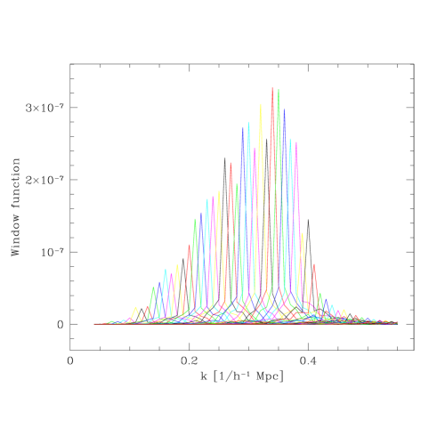
Figure 7.— The window functions are shown for the $130\>h^{-1}{\rm Mpc}$ volume-limited sample using the decorrelation method. The $i^{th}$ row of ${\bf W}$ typically peaks at the $i^{th}$ band, the scale $k$ that the band power estimator $\widehat{p}_{i}$ was designed to probe. To facilitate comparison with Figure 6, we have rescaled the window functions to sum to $(\Delta{\bf p}_{i})^{-2}$ rather than unity here.

The two above-mentioned choices for ${\bf M}$ both tend to produce correlations between the band power error bars. The minimum-variance choice generally gives positive correlations, since the Fisher matrix cannot have negative elements, whereas the unbiased choice tends to give anticorrelation between neighboring bands. The choice (Tegmark & Hamilton 1998; Hamilton & Tegmark 2000)

$${\bf M}_{ij}=\left[\sum_{j=1}^{{N_{p}}}\left({\bf F}^{-1/2}\right)_{ij}\right]^{-1}\left({\bf F}^{1/2}\right)_{ij},$$ (26)

i.e., ${\bf M}={\bf F}^{-1/2}$ with the rows renormalized, has the attractive property of making the errors uncorrelated, with the covariance matrix of equation (23) diagonal. The corresponding window functions ${\bf W}$ are plotted in Figure 7, and are seen to be quite well-behaved, even narrower than those in Figure 6 while remaining positive. This choice is a compromise between the two first ones: it narrows the minimum variance window functions at the cost of only a small noise increase, with uncorrelated noise as an extra bonus. Note that all three choices of ${\bf M}$ retain all the cosmological information, since the vector ${\bf y}$ can always be recovered by multiplying $\widehat{\bf p}$ by ${\bf M}^{-1}$. The minimum-variance band power estimators are essentially a smoothed version of the uncorrelated ones, and their lower variance was paid for by correlations which reduced the effective number of independent measurements.

3.5. Integral constraint correction

Since the main focus of this paper is the power spectrum on the largest scales, it is crucial that we deal with the complication known as the integral constraint (Peacock & Nicholson 1991). If we knew the selection function ${\bar{n}}({\bf r})$ a priori, before counting the galaxies in our survey, we would be able to measure the power on the scale of the survey. Our power spectrum estimate would essentially be the square of the ratio of the observed and expected number of galaxies in our sample. Of course, we do not know ${\bar{n}}$ a priori, so we use the galaxies themselves to normalize the selection function. Thus the measured density fluctuation automatically vanishes on the scale of the survey, and and naïve application of the power spectrum estimation method we have described will falsely indicate that $P(k)\to 0$ as $k\to 0$, regardless of the behavior of the true power spectrum on large scales.

Fortunately, this problem has a simple remedy once the data has been pixelized. As described in T98, the problem is that we do not know the true amplitude of the mean density mode $\bf m$ defined in equation (3), and consequently may not have subtracted it out correctly in equation (2). We can therefore immunize our data to this problem by making it orthogonal to $\bf m$. Defining a projection matrix

$${\bf\Pi}\equiv{\bf I}-{\bf m\bf m^{t}\over|\bf m|^{2}},$$ (27)

the recipe is simply to replace ${\bf x}$ by ${\bf\Pi}{\bf x}$ and the matrices ${\bf C},_{i}$ by ${\bf\Pi}{\bf C},_{i}{\bf\Pi}$ (T98). This trick of choosing modes that are orthogonal to the mean density was first suggested by Fisher et al. (1993). We find that this correction increases our error bars slightly on the largest scales, mainly in the leftmost band.

4. Results

4.1. Basic results

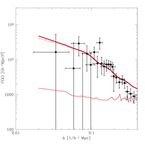
Figure 8.— Decorrelated band-power measurements are shown for the $101\>h^{-1}{\rm Mpc}$ volume-limited sample. Although the window functions overlap slightly, the errors are all uncorrelated. The error bars include the effects of both shot noise and sample variance corresponding to the fiducial model. The horizontal bars show the rms width of the window function corresponding to each measurement. If the fiducial model (heavy curve) is correct, the measurements should on average equal this curve convolved with the window functions (dotted curve). The thin red line shows the shot noise contribution that has been subtracted out.

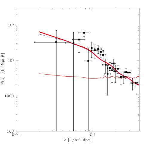
Figure 9.— Same as previous figure, but for the $130\>h^{-1}{\rm Mpc}$ volume-limited sample.

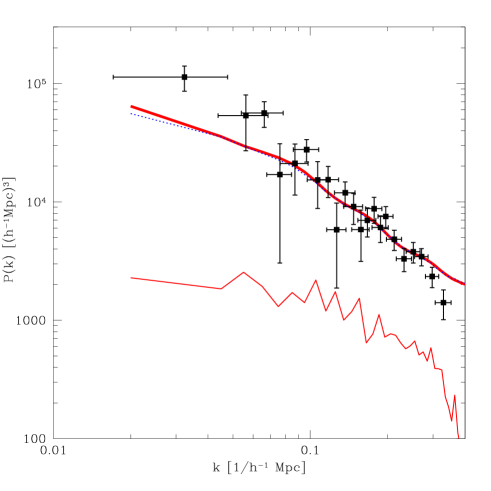
Figure 10.— Same as previous figure, but for the magnitude limited sample.

Our basic results are shown in Figures 8, 9 and 10. Here the band power estimates are computed using the ${\bf M}$-choice of Section 3.4.3, so the error bars are uncorrelated. The horizontal location of each data point and the width of the horizontal bars are the mean and the standard deviation of the corresponding window function, respectively. To avoid excessive clutter, we have averaged neighboring band-power measurements (and their corresponding window functions) on the smallest scales using a simple inverse-variance weighting since the error bars are uncorrelated.

The heavy curve shows the prior power spectrum vector ${\bf p}$ that was used in the calculation. It is a flat $\Lambda$CDM “concordance model” (Wang et al. 1999) with $\Omega_{\Lambda}=0.7$, $\Omega_{cdm}=0.25$, $\Omega_{b}=0.05$, $h=0.65$, $n=1$ with $\sigma=1$ for the matter fluctuations, rescaled by a different bias factor for each of the three galaxy samples. The linear power spectrum for this model was computed using the fit of Eisenstein & Hu (1999), then corrected for nonlinear effects with the formalism of Jain et al. (1995) based on HKLM scaling (Hamilton et al. 1991; Peacock & Dodds 1996), with the local power spectrum slope given by the “baryon wiggle-free” version of the spectrum. Our non-linear $\sigma_{8}=1$ normalization corresponds to a linear $\sigma_{8}\approx 0.93$. We first estimated a power spectrum assuming $b=1$, then iterated the calculation once with new bias factors providing a better normalization to the actual measurements. For the $101\,h^{-1}{\rm Mpc}$, $130\,h^{-1}{\rm Mpc}$ and magnitude-limited samples, these three bias factors $b$ (reflected by the heavy curves shown in Figures 8, 9 and 10) are 1.2, 1.4 and 1.4, respectively.

This is not a complete treatment of non-linearity (see, e.g., Meiksin & White 1999; Scoccimarro et al. 1999; Hamilton 2000; Benson et al. 1999). The effects of nonlinearity will not bias our power spectrum estimates, but the error bars are likely to be underestimated on nonlinear scales $k\mathrel{\hbox to0.0pt{\lower 3.0pt\hbox{$\mathchar 536\relax$}\hss}\raise 2.0pt\hbox{$\mathchar 318\relax$}}0.3/h^{-1}{\rm Mpc}$.

Since each data point is the power spectrum convolved with a window function, we would not expect the data points to fall exactly on the true power spectrum even on average. Rather, if the prior were correct, they would on average fall on the dotted curve ${\bf W}{\bf p}$, which shows the prior averaged with the window functions of each band. In all cases, the results are seen to be consistent with the priors used, except perhaps on the very smallest scales and for the leftmost band in the magnitude-limited case, to which we will return in Section 4.5 below. We will discuss robustness towards the choice of prior below in Section 4.3.1.

How reliable are these results? In the remainder of this section, we present a series of tests, both of our software and algorithms and of potential systematic errors.

4.2. Validation of method and software

Since our analysis consists of a number of somewhat complicated steps, it is important to test both the software and the underlying methods. We do this by generating $N_{\rm monte}=200$ Monte Carlo simulations of the UZC catalog with a known power spectrum, processing them through our analysis pipeline and checking whether they give the correct answer on average and with a scatter corresponding to the predicted error bars. We found this end-to-end testing to be quite useful in all phases of this project — indeed, things worked on neither the first nor the second attempt…

4.2.1 The mock survey generator

Standard N-body simulations would not suffice for our precision test, because of a slight catch-22 situation: the true non-linear power spectrum of which an N-body simulation is a realization (with shot noise added) is not known analytically, and is usually estimated by measuring it from the simulation — but this is precisely the step that we wish to test. We therefore resort to a simpler approach, where we generate realizations that are still in the linear regime, just as is routinely done when preparing initial conditions for N-body simulations. We do this in the following steps:

1. Generate a Gaussian random field with the prescribed power spectrum on a cubic grid (by generating uncorrelated Gaussian random variables with variance $P(k)$ at each grid point in Fourier space, then performing an FFT).

2. Generate a random galaxy position ${\bf r}_{i}$ inside the angular mask with radial probability distribution prescribed by the selection function.

3. Evaluate the density field $\delta$ at ${\bf r}_{i}$ using trilinear interpolation between the nearest points on the FFT grid.

4. Add this galaxy to the catalog with a probability equal to $[1+\delta({\bf r}_{i})]/2$, otherwise discard it.

5. Go back to step 2 and repeat until the desired number of galaxies has been generated.

To avoid the quantity $1+\delta({\bf r}_{i})$ going negative in step 4, which would spoil our procedure, we normalize our fiducial power spectrum to have much less power than observed in the actual Universe. We choose our test power spectrum to be a simple Gaussian $P(k)\propto e^{-(Rk)^{2}/2}$ with $R=32\,h^{-1}{\rm Mpc}$, normalized so that the rms fluctuations $\langle\delta^{2}\rangle^{1/2}=0.2$. This ensures that $|\delta|>1$ (breaking step 4) occurs only a negligible fraction of the time (about once in 1.7 million).

4.2.2 Testing the Heavens-Taylor pixelization

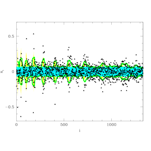
Figure 11.— The triangles show the elements $x_{i}$ of the data vector ${\bf x}$ (the HT expansion coefficients) averaged over 200 Monte-Carlo simulations of the $101\>h^{-1}{\rm Mpc}$ volume-limited sample. If the algorithms and software are correct, then their mean should be zero and about $68\%$ of them should lie within the shaded yellow/grey region giving their standard deviation. The green/grey curve is the rms of the data points $x_{i}$, averaged in bands of width 25, and is seen to agree well with a smoothed version of the shaded region.

Figure 11 shows the result of processing the Monte Carlo simulations through the first step of the analysis pipeline, i.e., computing the corresponding Heavens-Taylor expansion coefficients $x_{i}$. This is a very sensitive test of the mean correction given by equation (3), which can be a couple of orders of magnitude larger than the scatter in Figure 11 for some modes. A number of problems with the radial selection function integration and the spherical harmonic expansion of the angular mask in our code were discovered in this way. After fixing these problems, the coefficients $x_{i}$ became consistent with having zero mean as seen in the figure. The figure also shows that the scatter in the modes is consistent with the predicted standard deviation $\sigma_{i}=({\bf C}_{ii}/N_{\rm monte})^{1/2}$ (shaded region), with most of the the fluctuations being localized to modes probing large scales (with $\ell$, $m$ and $n$ being small).

Processing the Monte Carlo simulations through the second step of the analysis pipeline showed that the corresponding KL eigenmodes $y_{i}$ passed the same test.

4.2.3 Testing the quadratic band-power estimation

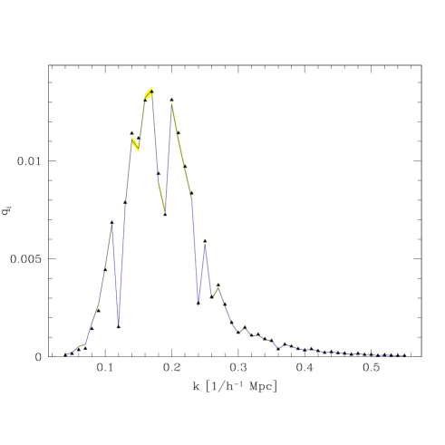
Figure 12.— The triangles show the elements $q_{i}$ of the raw quadratic band-power estimators ${\bf q}$, averaged over 200 Monte-Carlo simulations of the $101\>h^{-1}{\rm Mpc}$ volume-limited sample. If the algorithm and the software is correct, then about $68\%$ of them would be expected to lie within the shaded yellow/grey band, centered on the solid curve.

Figure 12 shows the result of processing the Monte Carlo simulations through the third step of the analysis pipeline, i.e., computing the raw unnormalized quadratic band-power estimates $q_{i}$. Since information from large numbers of modes contributes to each $q_{i}$, the scatter $\sigma_{i}=({\bf F}_{ii}/N_{\rm monte})^{1/2}$ is seen to be small. Therefore, even quite subtle bugs and inaccuracies can be (and were!) discovered and remedied as a result of this test.

4.2.4 Testing the Fisher decorrelation

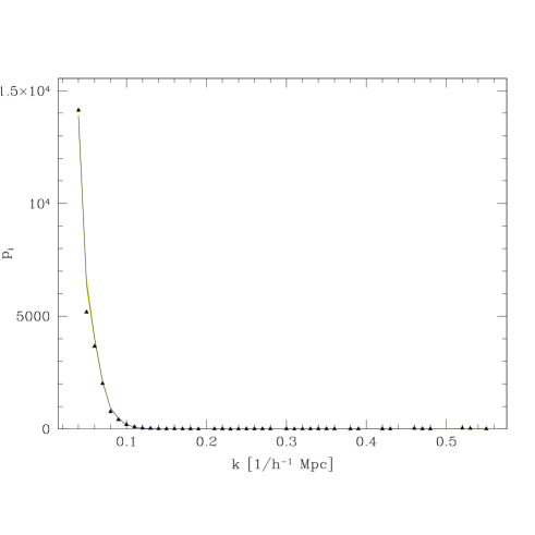
Figure 13.— The triangles show the decorrelated band-power estimates $\widehat{p}_{i}$, averaged over 200 Monte-Carlo simulations of the magnitude-limited sample. If the algorithm and the software is correct, then about $68\%$ of them should lie within the shaded yellow/grey band, centered on the Gaussian fiducial power spectrum (solid curve).

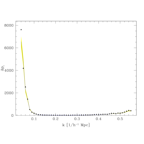
Figure 14.— Same as the previous figure, but for the error bars $\Delta p_{i}$. The triangles show the observed scatter in the 200 simulations. If the algorithm and the software is correct, then about $68\%$ of them should lie within the shaded yellow/grey band predicted by the Fisher matrix formalism, centered on the solid curve.

Figures 13 and 14 show the result of processing the Monte Carlo simulations through the fourth and final step of the analysis pipeline, i.e., computing the decorrelated and normalized band-power estimates $p_{i}$. The mean recovered power spectrum is seen to be in excellent agreement with the Gaussian prior used in the simulations (Figure 13) convolved with the window functions, and the observed scatter is seen to be consistent with the predicted error bars (Figure 14). These two figures therefore constitute an end-to-end test of our data analysis pipeline, since errors in any of the many intermediate steps would have shown up here at some level.

4.3. Robustness to method details

Our analysis pipeline has a number of “knobs” that can be set in more than one way. This section discusses the sensitivity to such settings.

4.3.1 Effect of changing the prior

Figure 15.— Effect of prior. The triangles show the decorrelated band-power estimates $p_{i}$, averaged over 200 Monte-Carlo simulations of the magnitude-limited sample with a Gaussian power spectrum (red line). The power spectrum estimation was carried out assuming a totally different fiducial model, the $\Lambda$CDM model to the right. If the data was consistent with the prior, about 68% of the measurements should fall within the narrow yellow/grey region. Instead, the method is seen to faithfully reproduce the actual input power spectrum, with no evidence of a bias towards the assumed prior.

The analysis method employed assumes a “prior” power spectrum via equation (10), both to compute band power error bars and to find the galaxy pair weighting that minimizes them. As mentioned, an iterative approach was adopted starting with a simple $\Lambda$CDM model with $\sigma_{8}=1$, then rescaling it to better fit the resulting measurements and recomputing the measurements a second time. To what extent does this choice of prior affect the results? On purely theoretical grounds (e.g., Tegmark, Taylor & Heavens 1997), one expects a grossly incorrect prior to give unbiased results but with unnecessarily large variance. If the prior is too high, the sample-variance contribution to error bars will be overestimated and vice versa. This hypothesis has been extensively tested and confirmed in the context of power spectrum measurements from the Cosmic Microwave Background (e.g., Bunn 1995). An analogous test is shown in Figure 15, showing that the correct result is recovered even when our 200 simulations are analyzed with a grossly incorrect prior.

Generally, the pair weighting strives to minimize the joint contribution from sample variance and shot noise to the scatter in the measurements. This scatter will therefore be unnecessarily large both if the prior is too low (so that sample variance not taken seriously enough) and if it is too high (so that excessive paranoia about sample variance gives a pair weighting producing unnecessarily large shot noise). The resulting scatter therefore increases only to second order when the prior is slightly off. Since the iterated priors used in our analysis of the real data agree so well with the actual measurements, slight remaining deviations of the prior from the truth are therefore likely to have a negligible impact.

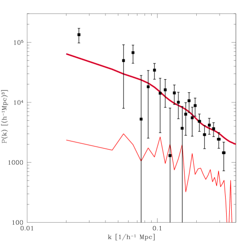
Figure 16.— Same as Figure 10 (magnitude-limited sample), but for the method giving maximally narrow window functions.

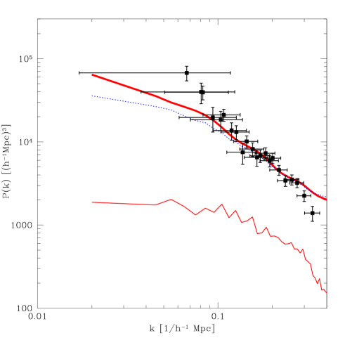
Figure 17.— Same as Figure 10 (magnitude-limited sample), but for the method giving smaller, bandwidth independent error bars.

4.3.2 Effect of changing the decorrelation method

Our main results for the power spectra (Figures 8–10) were computed using the decorrelation method given by equation (26). To assess the sensitivity to this choice, we repeated the analysis for the other methods. The results were generally consistent with the same fiducial models, but as expected, the nature of the scatter was found to be strongly method-dependent. This is illustrated in Figures 16 and 17 for the magnitude-limited case.

Figure 16 used the method given by equation (25), giving maximally narrow window functions. Although they are plotted as having zero width, a calculation with narrower bands would show them to have a width of order that of the bands used here, i.e., of order the horizontal separation between neighboring points on the plot. However, Figure 16 also shows that there are no free lunches: the errors are bigger than in Figure 10, and the error covariance matrix shows that they are strongly anti-correlated with their nearest neighbors. This figure is essentially a window-deconvolved version of Figure 10, and smoothing it would recover that figure.

Figure 17 used the method given by equation (24), and deviates from Figure 10 in the opposite way from the previous example. It is essentially a smoothed version of Figure 10, giving nice small error bars, slightly broader window functions and positively correlated errors between neighboring points. The broader window functions are seen to be particularly annoying on the largest scales, where they shift the effective wavenumber probed far to the right.

4.3.3 Effect of changing the galaxy weighting

When expanding our galaxies in HT modes, we applied the radial FKP weighting given by equation (9). How does this particular choice affect the results? To address this issue, we repeated the analysis with equation (9) replaced by $w(r)\propto{\bar{n}}(r)$, i.e., the simple $P(k)=0$ limit of equal weight per galaxy. This resulted in almost no perceptible loss of information, typically increasing the band-power error bars on large scales by less than a percent. The resulting power spectrum measurements were essentially unchanged.

In the limit where infinitely many HT modes would be used, any functions whatsoever can be created by taking linear combinations of them, since they form a complete basis over the survey volume. This would make the choice of the radial weighting function $w(r)$ completely irrelevant, since the subsequent KL compression step would end up recovering the true KL eigenfunctions regardless. The reason that the radial weighting makes any difference at all in our case is therefore that we have used only a limited number of modes to start with, making it important that they do not grossly over- or underweight sparse distant galaxies relative to nearby ones.

4.3.4 Effect of other method details

The analysis above was performed using $11^{3}=1331$ HT modes, with an angular cutoff at $\ell_{\rm max}=10$ giving $(1+\ell_{\rm max})^{2}=121$ angular modes $Y_{\ell m}$ and a radial cutoff $n_{\rm max}=10$ giving 11 radial modes $j_{\ell}(k_{\ell n}r)$ per $Y_{\ell m}$. To explore the sensitivity to these choices, we repeated the entire analysis with $\ell_{\rm max}=n_{\rm max}=$ 3, 5 and 7 giving 64, 216 and 512 HT modes, respectively. As expected, we found that the band powers on the very largest scales converged quite rapidly as more modes were added, and that the new information made a difference mainly on the smaller scales where the new modes were sensitive. These numerical experiments suggested that our 1331 mode analysis retained a large fraction of the cosmological information down to $k\sim 0.3$, and that a more ambitious analysis with more modes would give substantially smaller error bars at smaller scales. The information matrix plotted in Figure 6 reenforces this conclusion.

To determine the best tradeoff between angular and radial modes, we performed a number of tests with $\ell_{\rm max}\neq n_{\rm max}$, keeping the total number of modes $(1+\ell_{\rm max})^{2}(1+n_{\rm max})$ roughly constant. These tests indicated that the largest Fisher information (the smallest error bars) on the power spectrum on the largest scales was obtained for the symmetric case $\ell_{\rm max}\sim n_{\rm max}$. This is why we used $\ell_{\rm max}=n_{\rm max}$ in our main analysis.

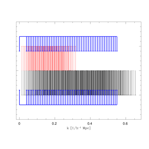
Figure 18.— Our 52 k-bands are shown (top and bottom) together with the discrete spectra of wavenumbers $k_{\ell m}$ used in the HT formalism. Of the two spectra, the upper one corresponds to the values $k_{\ell m}$ used in equation (8) for expanding the data, whereas the lower one corresponds to the values used in equation (10) for computing the covariance matrix ${\bf C}$ and its derivatives ${\bf C},_{i}$, both for the magnitude limited analysis.

We used 52 $k$-bands as illustrated in Figure 18. To compute the covariance matrix ${\bf C}$ and its 52 derivatives ${\bf C},_{i}$ exactly using equation (10), the contributions from a very large set of $k_{\ell m}$-values would be required. In practice, we truncated the $k_{\ell m}$-values used for these internal computations (the lower subset in Figure 18) at $\ell=\ell_{\rm max}=21$, since experimentation with different cutoff values $\ell_{\rm max}$ showed that all results for $k\mathrel{\hbox to0.0pt{\lower 3.0pt\hbox{$\mathchar 536\relax$}\hss}\raise 2.0pt\hbox{$\mathchar 316\relax$}}0.3$ had converged by then. An alternative approach to truncation is to make a sharp cut at a fixed $k$-value (HT).

As mentioned above, equation (10) is only approximate. The discrete spectra shown in Figure 18 would apply only if the radial Bessel functions were allowed to extend to infinite radius. Since they are truncated outside the survey volume, the sharp lines of Figure 18 get slightly smeared out: they essentially get convolved with the Fourier transform of the survey volume, which gives them a characteristic width $\Delta k$ of order the inverse size of the survey volume.

In the eigenmode expansion, the cutoff was placed at an ${\bf S}$-eigenvalue of $10^{-6}$, simply to avoid numerical singularities. This reduced the original 1331 modes to 1182, 1166 and 1206 for the $101h^{-1}{\rm Mpc}$, $130h^{-1}{\rm Mpc}$ and magnitude limited samples, respectively. The results remained completely unchanged when this $10^{-6}$ cutoff was increased by two orders of magnitude. Since 1331 models are very manageable numerically, our principal motivation for performing the subsequent S/N-analysis was to check for systematic errors. We therefore discarded no further modes in this step.

4.4. Robustness to extinction

Mis-estimates of ${\bar{n}}$ constitute a potential source of systematic errors. Although our method for dealing with the integral constraint immunized against errors in the overall normalization of ${\bar{n}}$, errors in its shape would still add spurious power to our estimate of $P(k)$. Let us first consider errors in the angular part of ${\bar{n}}$ caused by Galactic dust, returning to errors in the radial part in the next subsection.

The angular modulations caused by dust extinction tend to have a power spectrum rising sharply towards the largest scales (Vogeley 1998), and is therefore of particular concern for the interpretation of our leftmost bandpower estimates. Although the UZC subset we are using is 98% complete relative to the underlying Zwicky sample, extinction can of course cause completeness modulations in the latter. To estimate the severity of this effect, we used the recent extinction map produced by Schlegel, Finkbeiner & Davis (1999), using their B-band conversion factor of 4.325.

The expected extinction in the regions relevant to the UZC survey is shown in Figure 19, and the data set is shown in the same projection in Figure 20 for comparison. In the northern sample, the extinction ranges from $\Delta m=$0.012 to 1.7 with a median of 0.11. The cleanest spot in the southern sample has $\Delta m=$0.061, and the extinction gets as extreme as $\Delta m=$63 in the Galactic plane (which we masked out).

To get a first crude handle on the importance of extinction, we applied our analysis separately to the relatively clean north and to the full, uncropped south (for this test, we used the regions delimited by solid lines in Figure 20, not the dashed lines). Perhaps surprisingly, the South does not show a great power excess over the North even though the whopping extinction associated with the Galactic plane was included in this southern sample. This is presumably due to a combination of effects: The calculations of Vogeley (1998) suggested that extinction (for the SDSS region in the north) would dominate over the cosmological power spectrum only on scales $k\mathrel{\hbox to0.0pt{\lower 3.0pt\hbox{$\mathchar 536\relax$}\hss}\raise 2.0pt\hbox{$\mathchar 316\relax$}}0.03/h^{-1}{\rm Mpc}$, and the smaller volume of the UZC survey precludes us from effectively probing such large scales. Also, although extinction is severe near the Galactic plane, this is a relatively smooth feature and therefore does not greatly affect smaller scale fluctuations.

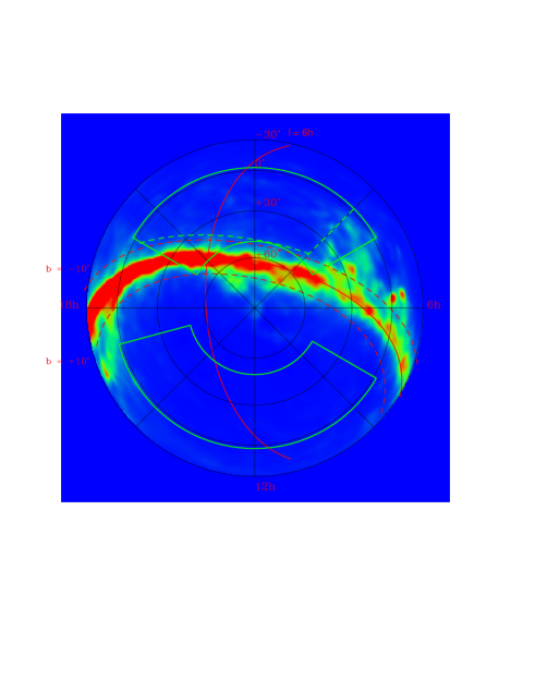
Figure 19.— The extinction $\Delta m$ predicted by Schlegel, Finkbeiner & Davis (1999) is shown in gnomonic equal-area projection with the North Celestial Pole in the center and right ascension $\alpha=0$ at the top, increasing clockwise. The Galactic plane is seen to intersect parts of the southern survey region. Note that the South Galactic Hemisphere is at the top.

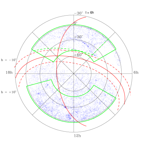
Figure 20.— The UZC galaxies are shown in the same coordinates as Figure 19. Note the visible deficit of galaxies in regions near the Galactic plane where Schlegel et al (1999) predict high extinction.

Indeed, the power spectrum in the North is, if anything, somewhat greater than in the South. This agrees with the findings of Park et al. and da Costa et al. (1994), reflecting the fact that the nearby southern sky is more quiescent, lacking northern structures such as Virgo and the Great Wall.

To be cautious, we nonetheless subjected the southern subsample to two additional cuts based on the dust map in Figure 19 before producing our main results, the power spectra shown in Section 4.1. Following Park et al. (1994), we moved the $4^{h}$ right ascension cut to $3^{h}$. We also excluded the region less than $13^{\circ}$ from the Galactic plane. Since the north-south differences were relatively minor without these cuts, we expect extinction to play only a subdominant role in this cropped data set.

We also corrected the observed magnitudes with the Schlegel et al. map and considered creating a new magnitude-limited sample for analysis. Unfortunately, this would have reduced the galaxy count too drastically to be of much interest. Since the extinction gets as high as $\Delta m=1.7$ even in the north, the new magnitude cut would have to be shifted from 15.5 to 13.8 to ensure completeness, leaving only $8\%$ of the galaxies from the original sample.

4.5. Robustness to radial selection function errors

To assess the extent to which radial selection function errors may be adding spurious power, we repeated our analysis with a variety of different selection functions. We replaced our Schecter parameters $(-1.1,-19.3)$ by a grid in $(\alpha,M_{*})$-space, always normalizing to match the observed number of galaxies. This had a substantial effect on the measured band powers, especially on the largest scales. We experimented with an iterative approach whereby the selection function was fine-tuned to minimize the large-scale power, but this unfortunately failed to converge: by grossly over-estimating the (small) number of distant galaxies, this procedure causes $\delta\equiv(n/{\bar{n}}-1)\to-1$, and since this function is spatially constant, it gives very little large-scale power. We therefore retained the radial selection function corresponding to the Schecter parameters measured from the data in the conventional way (de Lapparent et al. 1989) in our quoted results above. However, in light of the sensitivity of the results to slight changes in the assumed luminosity function, the leftmost bandpower measurement should be taken with a liberal dash of salt. In particular, the suspiciously high value seen at $k\sim 0.03/h^{-1}{\rm Mpc}$ for the $130h^{-1}{\rm Mpc}$ sample in Figure 9 may well be due to this effect. Selection function problems may be present even in the nominally volume-limited surveys, since Malmquist bias produces a selection function that is not quite constant near the far edge of the survey volume.

5. Conclusion

We have computed the redshift space power spectrum of the UZC galaxy redshift catalog. The results are summarized in Figures 8-10 and are well fit by, e.g., a $\Lambda$CDM model with a moderate amount of bias (1.2 to 1.4).

This paper is part of a larger effort to make galaxy redshift survey analysis more comparable to the state of the art for CMB experiments, explicitly calculating the window function for each band power measurement and including all finite-volume effects in the quoted error bars. However, it is merely the first step, and much work remains to be done:

1. We measured only the power spectrum in redshift space. A more ambitious analysis should extract the additional information present in clustering anisotropies due to redshift-space distortions.

2. We focused only on large scales, optimizing our pair weighting for the case of Gaussian fluctuations. For future work on smaller non-linear scales, $k\sim 0.3/h^{-1}{\rm Mpc}$, better results can be obtained by modeling the non-negligible correlations between different ${\bf k}$-modes that have been observed in simulations (Meiksin & White 1999; Scoccimarro et al. 1999; Hamilton 2000).

3. We measured merely the galaxy power spectrum. A more ambitious analysis would attempt to model the biasing issues needed to translate this into a measurement of the underlying matter power spectrum, for instance by combining the stochastic biasing formalism (Pen 1998; Dekel & Lahav 1999; Tegmark & Peebles 1998; Somerville et al. 2000) with redshift space distortions as outlined in Tegmark (1998) and/or by studying higher-order moments.

4. Given the sensitivity of the results to errors in the radial selection function, it would be worthwhile for a future analysis to include a likelihood analysis of its shape (Binggeli et al. 1988; Willmer 1997; Tresse 1999).

5. It is likely that model testing with future large surveys will require detailed Monte Carlo simulations to quantify and correct for subtle survey selection effects (e.g., fiber collisions). Fortunately, the matrix-based analysis pipeline we have presented lends itself well to this: once the Fisher matrix has been computed, the time required to analyze another (Monte Carlo) survey scales merely as $N_{x}^{2}$, not as $N_{x}^{3}$.

6. Our clustering analysis was limited to the power spectrum, i.e., to second moments of the density field. Higher-order moments of the density field are likely to contain a wealth of additional cosmological information on small scales (see Frieman & Gaztañaga 1999 and references therein).

These are major challenges, but the unprecedented quality of the impending data sets from ongoing redshift surveys such as 2dF and SDSS provide ample motivation to pursue them.

Acknowledgements: We thank Emilio Falco, Eric Gawiser, Andy Taylor and Jeffrey Willick for useful discussions, the UZC team for kindly making their data public, and John Bahcall and Jeffrey Willick for helping to organize a summer visit for N.P. to the Institute for Advanced Study during which much of this work was carried out. N.P. and A.J.S.H. both appreciated the hospitality of the IAS. N.P. was supported by a President’s Scholar Grant from Stanford University. M.T. was supported by the Alfred P. Sloan Foundation and by NASA though grant NAG5-9194 and Hubble Fellowship HF-01084.01-96A from STScI (operated by AURA, Inc. under NASA contract NAS5-26555). A.J.S.H. was supported by NASA grant NAG5-7128.

REFERENCES

Benson, A. J., Cole, S., Frenk, C. S., Baugh, C. M., & Lacey, C. G. 2000, MNRAS, 311, 793

Binggeli, B., Sandage, A., & Tammann, G. A. 1988, ARA&A, 26, 509

Bond, J. R. 1995, Phys. Rev. Lett., 74, 4369

Bond, J. R., Efstathiou, G., & Tegmark, M. 1997, MNRAS, 291, L33

Bond, J. R., Jaffe, A. H., & Knox, L. E. 2000, ApJ, 533, 19

Bunn, E. F. 1995, Ph.D. Thesis, U.C. Berkeley

da Costa, L. N., Vogeley, M. S., Geller, M. J., Huchra, J. P., & Park, C. 1994, ApJL, 437, L1

Davis, M., Huchra J P, Lantham, D., & Tonry, J. 1982, ApJ, 253, 423

Dekel, A., & Lahav, O. 1999, ApJ, 520, 24

de Lapparent, V., Geller, M. J., & Huchra, J. F. 1989, ApJ, 343, 1

Eisenstein, D. J., Hu, W., & Tegmark M 1999, ApJ, 518, 2

Eisenstein, D. J., & Hu, W. 1999, ApJ, 511, 5

Falco, E. E. et al. 1999, PASP, 111, 438

Feldman, H. A., Kaiser, N. , & Peacock, J. A. 1994, ApJ, 426, 23

Fisher, K. B., Davis, M., Strauss, M. A., Yahil, A., & Huchra, J. P. 1993, ApJ, 402, 42

Fisher, K. B., Scharf, C. A., & Lahav, O. 1994, MNRAS, 266, 219

Frieman, J. A., & Gaztañaga, E. 1999, ApJL, 521, L83

Geller, M. J., & Huchra, J. P. 1989, Science, 246, 857

Geller, M. J., & Huchra, J. P., Vogeley, M. S., & Geller, M. J. 1999, ApJS, 121, 287

Girardi, M., Boschin, W., & da Costa, L. N. 2000, A&A, 353, 57

Gunn, J. E., & Weinberg, D. H. 1995, in Wide-Field Spectroscopy and the Distant Universe, eds. S. J. Maddox and A. Aragón-Salamanca (Singapore: World Scientific), 3

Heavens, A. F., & Taylor, A. N. 1995, MNRAS, 483, 497 (“HT”)

Hamilton, A. J. S. 1997a, MNRAS, 289, 285

Hamilton, A. J. S. 1997b, MNRAS, 289, 295

Hamilton, A. J. S., Kumar, P., Lu, E., & Mathews, A. 1991, ApJL, 374, L1

Hamilton, A. J. S. 2000, MNRAS, 312, 257

Hamilton, A. J. S., & Tegmark, M. 2000, MNRAS;312;285

Huchra, J. P., Davis, M., Lantham, D., & Tonry, J. 1983, ApJS, 52, 89

Huchra, J. P., Geller, M. J., de Lapparent, V., & II, G. Jr. 1.990, ApJS, 72, 433

Huchra, J. P., Geller, M. J., & Corwin, II. G. Jr. 1995, ApJS, 99, 391

Jain, B., Mo, H. J., & White, S. D. M. 1995, MNRAS, 276, L25

Karhunen, K. 1947, Über lineare Methoden in der
Wahrscheinlichkeitsrechnung (Kirjapaino oy. sana: Helsinki)

Marzke, R. O., Huchra, J. P., & Geller, M. J. 1994, ApJ, 428, 43

Matsubara, T., Szalay, A. S., & Landy, S. D. 2000, ApJ, 535, 1

Meiksin, A., & White, M. 1999, MNRAS, 308, 1179

Park, C., Vogeley, M. S., Geller, M. J., & Huchra, J. F. 1994, ApJ, 431, 569

Peacock, J. A., & Dodds, S. J. 1996, MNRAS, 280, 19

Peacock, J. A., & Nicholson, D. 1991, MNRAS, 253, 307

Pen, U. 1998, ApJ, 504, 601

Schlegel, D. J., Finkbeiner, D. P., & Davis, M. 1998, ApJ, 500, 525

Schmalzing, J., & Diaferio, A. 2000, MNRAS, 312, 638

Scoccimarro, R., Zaldarriaga, M., & Hui, L. 1999, ApJ, 527, 1

Somerville, R. S., Lemson, G., Sigad, Y., Dekel, A., Kauffmann, G., & White, S. D. M. 2000, astro-ph/9912073

Tadros, H. et al. 1999, MNRAS, 305, 527

Tegmark, M. 1997, Phys. Rev. D, 55, 5895 (“T97”)

Tegmark, M. 1998, astro-ph/9809185, in Wide Field Surveys in Cosmology, ed. Colombi, S., & Mellier, Y. (Editions Frontières: Paris)

Tegmark, M., & Hamilton, A. J. S. 1998, astro-ph/9702019, in Relativistic Astrophysics & Cosmology, ed. Olinto, A. V., Frieman, J. A., & Schramm, D. (World Scientific: Singapore), p270

Tegmark, M., Hamilton, A. J. S., Strauss, M. A., Vogeley, M. S., & Szalay, A. S. 1998, ApJ, 499, 555

Tegmark, M., & Peebles, P. J. E. 1998, ApJL, 500, 79

Tegmark, M., Taylor, A. N., & Heavens, A. F. 1997, ApJ, 480, 22

Tresse, L. 1999, astro-ph/9902209, in Formation and Evolution of Galaxies, ed. Le Fèvre, O., & Charlot, S. ( Springer: Berlin)

Vogeley, M. S. 1998, astro-ph/9805160, in Ringberg Workshop on Large-Scale Structure, ed. Hamilton, D. (Kluwer: Amsterdam)

Vogeley, M. S., & Szalay, A. S. 1996, ApJ, 465, 34

Wang, L., Caldwell, R. R., Ostriker, J. P., & Steinhardt, P. J. 2000, ApJ, 530, 17

Willmer, C. N. A. 1997, Astron. J, 114, 898

Zaldarriaga, M., Spergel, D. N., & Seljak, U. 1997, ApJ, 488, 1

This paper is available with figures and power spectrum data from
h t t p://www.physics.upenn.edu/$\sim$max/uzc.html