Obscuration model
of Variability in AGN

Abstract

There are strong suggestions that the disk-like accretion flow onto massive black hole in AGN is disrupted in its innermost part (10-100 Rg), possibly due to the radiation pressure instability. It may form a hot optically thin quasi spherical (ADAF) flow surrounded by or containing denser clouds due to the disruption of the disk. Such clouds might be optically thick, with a Thompson depth of order of 10 or more. Within the frame of this cloud scenario collin96 ; czerny98 , obscuration events are expected and the effect would be seen as a variability. We consider expected random variability due to statistical dispersion in location of clouds along the line of sight for a constant covering factor. We discuss a simple analytical toy model which provides us with the estimates of the mean spectral properties and variability amplitude of AGN, and we support them with radiative transfer computations done with the use of TITAN code of dumont99 and NOAR code of abrassart99 .

Introduction

The variability of radio quiet AGN has been established since the early EXOSAT observations. However, the nature of this variability, observed in the optical, UV and X-ray band is not clear.

The emission of radiation is caused by accretion of surrounding gas onto a central supermassive black hole. The observed variability may be therefore directly related to the variable rate of energy dissipation in the accretion flow. However, it is also possible that the observed variability does not represent any significant changes in the flow. Such an ’illusion of variability’ may be created if we do not have a full direct view of the nucleus. We explore this possibility in some detail.

Clumpy accretion flow has been suggested by various authors in a physical context of gas thermal instabilities or strong magnetic field (e.g. celotti92 ; krolik98 ; torricelli98 ). Here we follow a specific accretion flow pattern described by collin96 .

We assume that the cold disk flow is disrupted at the distance of 10 - 100 $R_{\rm Schw}$ from the black hole. The resulting clumps of cool material are large and optically very thick for electron scattering, and they become isotropically distributed around the central black hole. Hot plasma responsible for hard X-ray emission forms still closer to a black hole, perhaps due to cloud collision. We do not discuss the dynamics of cloud formation but we concentrate on the description of the radiation produced by such a system. We consider the radiative transfer within the clouds and radiative interaction between the clouds and a hot phase, and we relate the radiation flux and spectra to the variations in the cloud distribution.

Variability mechanism

Within the frame of the cloud scenario, our line of sight to the hot X-ray emitting plasma is partially blocked by the surrounding optically thick clouds. Variations in the cloud distribution lead to two types of phenomena: slower variations due to the systematic change in a total number of clouds and fastest variations due to the random rearrangement of the clouds without any change of their total number. We concentrate on this second type of variability.

The amplitude of such a variability is determined by the number of clouds $N$ surrounding a black hole at any given moment and the mean covering factor $C$ of the cloud distribution $\left({\delta L_{X}\over L_{X}}\right)_{obs}={C\sqrt{2/N}\over 1-C}$.

Such variations do not reflect any deep changes in the hot plasma itself so they are expected to happen without the change in the hard X-ray slope of the plasma emission. However, the UV variability amplitude caused by the same mechanism as well as some variations in hard X-rays due to the presence of the X-ray reflection depend in general on the cloud properties like X-ray albedo and radiative losses through the unilluminated dark sides of clouds. We use very detailed radiative transfer in X-ray heated optically thick clouds in order to estimate those quantities. We develop a complementary toy model describing the energetics of the entire hot plasma/cloud system for easy use to estimate the model parameters from the observed variability amplitudes.

Radiative transfer solutions for mean spectra

Two codes are used iteratively in order to compute a mean spectrum emitted by the clouds distribution. TITAN dumont99 is designed to solve the radiative transfer within an optically thick medium, including computations of the ionization state of the gas and its opacities. NOAR abrassart99 is a Monte Carlo code designed to follow the hard X-ray photons using Monte Carlo method.

Figure 1: The exemplary spectrum calculated with the coupled codes TITAN and NOAR for the following parameters of the shell: number density log$n=14$, column density log $N_{H}=26$, covering factor $C=0.9$. The incident primary radiation was assumed to be a power law extending from 1 eV to 100 keV, with energy index $\alpha=1$, and the ionization parameter $xi=300$. The size of the central source was neglected.

The result of the numerical computation of a single mean spectrum is shown in Figure 1. The cloud distribution was assumed to be spherical, with the covering factor $C=0.9$, all clouds being located at a single radius. The hot medium in this computation was replaced by a point like source of a primary emission, with flux normalizations fixed through specification of the ionization parameter $\xi$. However, the multiple scattering of photons of different clouds was included.

We see that the broad band spectrum clearly consists of two basic components but there are also detailed spectral features in UV and soft X-ray band in addition to hard X-ray iron $K_{\alpha}$ line.

Toy model and variability amplitudes

In our toy model we replace the radiative transfer computations with analytical description of the probabilities of the X-ray and UV photon fate. X-ray photons can be reflected by bright sides of the clouds, can escape from the central region towards an observer or can be absorbed and provide new UV photons as well as energy for the emission from the dark sides. UV photon can also escape, can be reflected and can be upscattered to an X-ray photon by a hot plasma. All those probabilities are determined by four model parameters: covering factor $C$, probability of Compton upscattering $\gamma$, X-ray albedo $a$ and efficiency of dark side emission $\beta_{d}$. The condition of compensating for the system energy losses with Compton upscattering relate those four quantities to the Compton amplification factor. The variability amplitude depends also on the number of clouds, $N$.

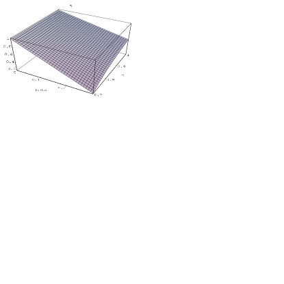
Figure 2: The dependence of the ratio of the normalized variability amplitude in $UV$ and in X-rays on the dark side loss eficciency $\beta_{d}$ and covering factor $C$; other parameters: X-ray albedo $a=0.5$, Compton amplification factor $A=4$.

Such a model allow us to calculate all basic properties of the stationary model, like the observed ratio of the X-ray luminosity to the UV luminosity, the intrinsic ratio of those two quantities as seen by the clouds, the slope of the hard X-ray emission and the variability amplitudes in UV and X-ray band.

In particular, we can determine the ratio of the normalized variability amplitudes in X-ray and UV band predicted by our model $R=\left({\delta L_{UV}\over L_{UV}}\right)_{obs}/\left({\delta L_{X}\over L_{X}}\right)_{obs}$. In Figure 2 we show the dependence of this ratio on the covering factor $C$ and the efficiency of the dark side energy loss by the clouds. The dependence on other model parameters was reduced by assuming the X-ray albedo $a=0.5$ supported by numerical results and the Compton amplification factor $A=4$ which well describes the mean hard X-ray spectral slope.

We see that if the clouds are very opaque ($\beta_{b}$ negligible) the normalized amplitude ratio is always equal 1 within the frame of our model. Significant dark side energy losses reduce the UV amplitude since they add a constant contribution to UV flux.

Discussion

The presented model well reproduces large observed variability amplitudes if the covering factor is close to 1. It also explains why large variability amplitudes are not necessarily accompanied by the change of the slope of the hard X-ray emission coming from comptonizing hot plasma. In order to check whether the model requires unacceptable values of the parameters we confront the model with the data in the following way.

We apply our toy model to observed variability of four Seyfert 1 galaxies extensively monitored in UV and X-ray band (see Table 1). The variability amplitudes are taken from goad99 ; edelson99 ; nandra98 ; edelson96 ; clavel92 , and we estimated the mean X-ray to UV luminosity ratio as 1/3 in all objects. We assumed the X-ray albedo $a=0.5$ and the Compton amplification factor as $A=4$. We calculated the remaining model parameters: $C$, $N$, $\gamma$, $\beta_{d}$.

All four objects are consistent with the model, having relative UV amplitude smaller than the relative X-ray amplitude. As expected, the covering factor (determined by the luminosity ratio) is large and the probability of Compton upscattering is low either due to small optical depth of the hot plasma or due to small radial extension of the hot plasma. The required dark side losses are comparable to the value of 0.20 obtained from the numerical solution of the radiative transfer within a cloud (see Figure 1). Therefore cloud scenario offers an attractive explanation of the observed variability of AGN if further observations will confirm that the slope of the direct Compton component and its high energy cut-off do not vary.

Table 1: Toy model parameters for AGN.

Object	$rms_{UV}$	$rms_{X}$	C	N	$\gamma$	$\beta_{d}$
NGC 3516	0.333	0.357	0.90	1180	0.047	0.04
NGC 7469	0.167	0.167	0.90	5400	0.044	0.00
NGC 4151	0.009	0.024	0.90	2610	0.095	0.39
NGC 5548	0.222	0.222	0.90	3050	0.044	0.00

References

- (1) Collin-Souffrin S., Czerny, B., Dumont, A.-M., and Życki, P.T., A&A 314, 393 (1996)
- (2) Czerny B., and Dumont A.-M., A&A, 338, 386 (1998)
- (3) Dumont A.-M., Abrassart A., and Collin S., A&A, (1999) (submitted)
- (4) Abrassart A., (1999) (in preparation)
- (5) Celotti, A, Fabian, A.C., and Rees, M., MNRAS, 255, 419 (1992)
- (6) Krolik, J.H., ApJ, 498, L13 (1998)
- (7) Torricelli-Ciamponi, G., and Courvoisier, T.J.-L., A&A, 335, 881 (1998)
- (8) Goad M.R., Koratkar A.P., Axon D.J., Korista K.T., O’Brien P.T.O, 1999, ApJ, 512, L95
- (9) Edelson R., and Nandra K., ApJ, 514, 682 (1999)
- (10) Nandra, K., Clavel, J., Edelson, R.A., George, I.M., Malkan, M.A., Mushotzky, R.F., Peterson, B.M., Turner, T.J., ApJ, 505, 594 (1998)
- (11) Edelson, R. et al. ApJ, 470, 364 (1996)
- (12) Clavel et al. ApJ, 393, 113 (1992)