Revised Strömgren metallicity calibration for red giants

Abstract

A new calibration of the Strömgren $(b-y),m_{1}$ diagram in terms of iron abundance of red giants is presented. This calibration is based on a homogeneous sample of giants in the globular clusters $\omega$ Centauri, M22, and M55 as well as field giants from the list of Anthony-Twarog & Twarog (anth98 (1998)). Towards high metallicities, the new calibration is connected to a previous calibration by Grebel & Richtler (greb92 (1992)), which was unsatisfactory for iron abudances lower than $-$1.0 dex. The revised calibration is valid for CN-weak/normal red giants in the abundance range of $-2.0<$[Fe/H]$<0.0$ dex, and a color range of $0.5<(b-y)<1.1$ mag.

As shown for red giants in $\omega$ Centauri, CN-weak stars with Strömgren metallicities higher than $-$1.0 dex cannot be distinguished in the $(b-y),m_{1}$ diagram from stars with lower iron abundances but higher CN band strengths.

1 Introduction

Strömgren photometry has been proven to be a reliable metallicity indicator for globular cluster giants and subgiants (e.g. Richtler rich89 (1989), Grebel & Richtler greb92 (1992) and references therein). The location of late type (G and K) giants in the Strömgren $(b-y),m_{1}$ diagram is correlated with their metallicities, especially with their iron and CN abundances. Whereas the color $(b-y)$ is not sensitive to metallicity, the Strömgren $v$ filter includes several iron absorption lines as well as the CN band at 4215Å, and therefore $m_{1}=(v-b)-(b-y)$ is a metallicity sensitive index (e.g. Bell & Gustafsson bell (1978)). Within a certain color range, $0.5<(b-y)<1.1$ mag, the loci of constant iron abundance of giants and supergiants can be approximated by straight lines. This is valid for CN-“normal” ($=$ CN-weak) stars. CN-strong stars, due to their higher absorption in the $v$ filter, scatter to higher $m_{1}$ values and therefore mimic a higher Strömgren metallicity than their actual iron abundance would correspond to. If a cluster is known to have only small star-to-star variations in its iron abundance, the scatter to higher $m_{1}$ values can be used to uncover CN-rich member stars. For giants redder than $(b-y)=1.1$ mag the calibration breaks down due to TiO and MgH absorption in the $y$ band.

Until now the calibration for Strömgren metallicities is based on the spectroscopically determined iron abundance of relatively metal-rich stars, and only few metal poorer stars (Grebel & Richtler greb92 (1992)). This calibration worked well for the determination of cluster abundances in the Magellanic Clouds (Hilker et al. 1995a , 1995b ; Dirsch et al. dirs (1999)), but failed to reproduce the slope of constant metallicity lines in the $(b-y),m_{1}$ diagram for the new data of metal poor globular clusters. Other previous metallicity calibrations in the Strömgren $(b-y),m_{1}$ plane have been published for the regime of F and G dwarfs (Schuster & Nissen schu (1989)) and F dwarfs and giants in the small color range of $0.22<(b-y)<0.38$ (Malyuto maly (1994)).

In the meantime, large samples of homogeneous spectroscopic measurements of cluster as well as field giants have become available. Furthermore, CCD Strömgren photometry, in particular in globular clusters, is becoming popular (e.g. Grundahl et al. grun99 (1999)). Therefore, a revised, more accurate calibration of the metallicity sensitive Ström- gren indices is needed. In this paper, the Strömgren metallicity calibration is extended to more metal-poor stars ([Fe/H] $>-2.0$ dex). The sample of stars used for the new calibration contains red giants of $\omega$ Centauri, M55, and M22, and field giants from a homogenized sample of Anthony-Twarog & Twarog (anth98 (1998)). $\omega$ Cen is known for its star-to-star variations in CN as well as iron abundances (e.g. Vanture et al. vant (1994)). For 40 giants in $\omega$ Cen, Norris & Da Costa (norr95 (1995)) measured accurate abundances from high resolution spectroscopy. M22 also shows CN abundance variations (e.g. Norris & Freeman norr82 (1982), norr83 (1983)). Both clusters have been used to study the influence of the CN band strengths on the Strömgren metallicity.

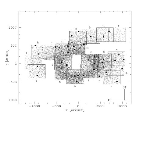
Figure 1: Position plot of the observed fields in $\omega$ Cen. All stars with a $V$ magnitude brighter than 19.0 mag and a photometric error less than 0.1 mag have been plotted. Filled circles indicate the position of the red giants with known spectroscopic abundances

Table 1: Position log of $\omega$ Cen fields

Id.	$\alpha_{2000}$	$\delta_{2000}$	Id.	$\alpha_{2000}$	$\delta_{2000}$
a	13:25:30.8	$-$47:26:46	k	13:28:12.9	$-$47:23:36
b	13:25:59.9	$-$47:17:46	l	13:28:27.0	$-$47:28:15
c	13:26:28.0	$-$47:27:46	m	13:27:18.0	$-$47:23:05
d	13:25:30.8	$-$47:31:16	n	13:26:50.0	$-$47:21:47
e	13:26:00.0	$-$47:32:27	o	13:26:47.0	$-$47:17:17
f	13:26:29.0	$-$47:32:27	p	13:26:16.9	$-$47:16:38
g	13:26:59.0	$-$47:34:56	q	13:25:46.9	$-$47:15:47
h	13:27:24.0	$-$47:33:06	r	13:25:29.9	$-$47:15:47
i	13:27:24.0	$-$47:28:34	s	13:25:30.8	$-$47:35:07
j	13:27:48.0	$-$47:24:05	t	13:28:15.9	$-$47:32:26

2 Observations and data reduction: $\omega$ Cen, M55, and M22

The observations were performed during the nights 21-24 April 1995 with the Danish 1.54m telescope at ESO/La Silla. The CCD in use was a Tektronix chip with 1024$\times$1024 pixels. The $f$/8.5 beam of the telescope provides a scale of $15\aas@@fstack{\prime\prime}7$/mm, and with a pixel size of 24 $\mu$m the total field is $6\aas@@fstack{\prime}3\times 6\aas@@fstack{\prime}3$. The observations and data reduction of the M22 and M55 images have been presented by Richter et al. (richp (1999)). In $\omega$ Cen, 20 fields were observed during the third night of the run through the Strömgren $ybv$ filters (Danish set of imaging filters). Table 1 gives a log of the field positions. In Fig. 1, all fields are plotted in a coordinate system centered on $\omega$ Cen. The exposure times were 70, 120, and 240 seconds for $y$, $b$ and $v$, respectively. All nights had photometric conditions, and the seeing, measured from the FWHM of stellar images, was in the range $1\aas@@fstack{\prime\prime}2-1\aas@@fstack{\prime\prime}5$.

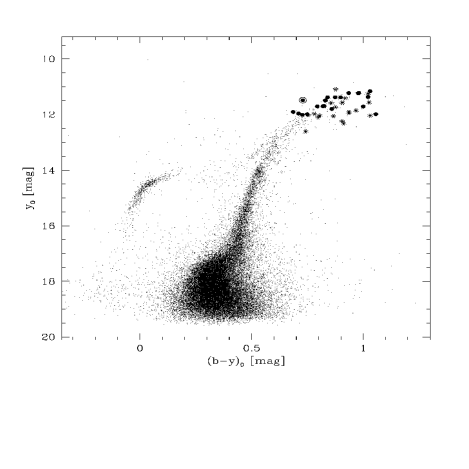
Figure 2: Color magnitude diagram of all stars in the observed fields (see Fig. 1) with photometric errors in all colors smaller than 0.1 mag. Filled circles indicate red giants from the spectroscopic sample with normal CN abundances, whereas red giants marked with asterisks are known to be CN-strong. The encircled dot is the star ROA 74 which deviates most from the metallicity calibration

The CCD frames were processed with standard IRAF routines. Instrumental magnitudes were derived using DAO- PHOT II (Stetson stet87 (1987), stet92 (1992)). For the comparison with the standard stars, aperture–PSF shifts have been determined in all fields. The remaining uncertainty of this shift is in the order of 0.01 mag in all filters. The corrected magnitudes of the stars belonging to overlapping areas of two adjacent fields agree very well and have been avaraged for the final photometry file. The calibration equations and coefficients for the third night are given in Richter et al. (richp (1999)).

Table 2: Photometric and spectroscopic data for red giants in $\omega$ Cen. All columns are explained in Sect. 3.1. A reddening of $E_{B-V}=0.11$ mag has been applied

ROA	$\Delta x$	$\Delta y$	$V_{0}$	$(b-y)_{0}$	$m_{1,0}$	[Fe/H]ph	[Fe/H]sp	CO	CN	C4142	S3839	CB
40	564.0	$-$89.0	11.088	0.876	0.484	$-$1.21	$-$1.69	$\circ$	…	…	0.46	0.34
42	$-$261.0	$-$56.0	11.409	0.919	0.506	$-$1.27	$-$1.69	…	$\circ$	0.32	0.50	…
43	696.5	897.9	11.249	1.022	0.671	$-$1.01	$-$1.47	$\circ$	…	0.34	0.42	0.31
46	$-$103.1	485.2	11.232	0.978	0.472	$-$1.57	$-$1.67	$\bullet$	$\bullet$	0.19	…	…
48	$-$230.1	316.8	11.219	0.980	0.422	$-$1.75	$-$1.76	$\bullet$	$\bullet$	..	…	0.19
53	878.1	$-$494.7	11.157	1.030	0.561	$-$1.40	$-$1.67	$\bullet$	$\bullet$	0.24	0.16	0.22
58	$-$236.0	486.5	11.376	0.874	0.396	$-$1.55	$-$1.73	$\bullet$	$\bullet$	0.21	0.16	0.22
65	369.5	188.0	11.225	0.935	0.369	$-$1.82	$-$1.72	…	$\bullet$	…	0.03	…
74	126.5	533.2	11.483	0.729	0.498	$-$0.52	$-$1.80	$\bullet$	$\bullet$	0.17	0.16	0.21
84	$-$85.7	389.2	11.565	1.026	0.708	$-$0.90	$-$1.36	$\circ$	…	0.30	0.17	0.30
91	6.4	889.4	11.491	0.830	0.329	$-$1.69	$-$1.73	$\bullet$	$\bullet$	…	0.07	0.16
94	572.8	108.9	11.379	0.840	0.330	$-$1.72	$-$1.78	…	$\bullet$	0.15	0.03	…
100	$-$259.6	$-$28.3	11.568	0.906	0.762	$-$0.25	$-$1.49	…	$\circ$	0.51	0.58	…
102	$-$929.1	$-$69.2	11.380	0.898	0.358	$-$1.77	$-$1.80	$\bullet$	$\bullet$	…	0.22	…
132	$-$90.7	$-$339.1	11.367	1.021	0.634	$-$1.13	$-$1.37	$\circ$	…	0.22	…	0.28
139	$-$435.2	437.5	11.585	0.856	0.618	$-$0.60	$-$1.46	$\circ$	$\circ$	0.39	…	0.52
144	$-$260.2	$-$61.0	11.980	0.781	0.473	$-$0.89	$-$1.66	…	$\circ$	0.33	…	…
155	994.8	$-$124.6	11.689	0.824	0.421	$-$1.28	$-$1.64	$\bullet$	$\bullet$	0.17	…	0.26
159	921.0	265.2	11.708	0.794	0.323	$-$1.60	$-$1.72	$\bullet$	$\bullet$	0.16	…	0.14
161	$-$515.7	461.7	11.697	0.819	0.396	$-$1.37	$-$1.67	$\bullet$	$\bullet$	0.14	…	0.26
162	$-$932.5	$-$328.7	11.851	0.967	0.965	$+$0.21	$-$1.10	$\bullet$	$\circ$	0.54	…	0.49
171	634.0	$-$233.5	11.727	0.875	0.548	$-$0.94	$-$1.43	$\circ$	$\bullet$	0.18	…	0.31
179	$-$379.6	43.2	11.710	1.000	0.710	$-$0.81	$-$1.10	$\circ$	…	0.18	…	0.29
182	$-$72.8	$-$340.3	11.800	0.859	0.515	$-$1.03	$-$1.46	…	…	0.23	…	…
201	224.4	105.0	11.984	1.056	0.692	$-$1.05	$-$0.85	…	…	…	…	0.28
213	281.7	747.5	11.904	0.686	0.211	$-$1.76	$-$1.83	$\bullet$	$\bullet$	0.18	…	0.06
219	$-$896.1	269.1	11.922	0.934	0.639	$-$0.83	$-$1.25	$\circ$	…	0.20	…	0.32
231	355.7	$-$158.4	11.919	0.937	0.818	$-$0.18	$-$1.10	$\bullet$	$\circ$	0.40	…	0.33
234	$-$148.1	771.0	11.962	0.710	0.222	$-$1.79	$-$1.78	$\bullet$	$\bullet$	0.11	$-$0.33	0.06
248	122.4	$-$326.7	12.039	1.031	0.968	$-$0.06	$-$0.78	$\bullet$	…	0.42	0.51	0.39
252	573.5	741.2	11.983	0.749	0.250	$-$1.79	$-$1.74	…	$\bullet$	0.10	0.10	…
253	1031.6	116.0	12.014	0.753	0.599	$-$0.18	$-$1.39	$\bullet$	$\circ$	0.42	1.00	0.57
256	546.2	37.4	12.012	0.727	0.301	$-$1.47	$-$1.58	$\bullet$	$\bullet$	0.14	0.27	…
270	476.6	$-$347.5	12.055	0.866	0.655	$-$0.49	$-$1.22	$\circ$	…	…	0.57	0.39
279	$-$976.9	505.9	12.035	0.805	0.643	$-$0.26	$-$1.69	…	CH	0.35	1.15	0.59
287	832.0	97.4	12.098	0.797	0.546	$-$0.64	$-$1.43	$\circ$	$\circ$	0.23	0.58	0.42
357	366.3	5.9	12.236	0.905	0.877	$+$0.19	$-$0.85	$\bullet$	…	…	…	0.41
371	$-$41.0	$-$499.5	12.320	0.912	0.847	$+$0.04	$-$0.79	$\bullet$	…	0.46	0.54	0.39
480	$-$5.2	$-$327.8	12.611	0.742	0.797	$+$0.82	$-$0.95	$\bullet$	$\circ$	…	1.32	0.65

After the photometric reduction and calibration of the magnitudes, the average photometric errors for the red giants used in the metallicity calibration are 0.015 mag for $V$, 0.016 mag for $(b-y)$ and 0.024 mag for $m_{1}$.

3 Sample of red giant stars

This section presents the sample of red giants that has been used for our new metallicity calibration. The spectroscopically determined iron abundances of the different authors are all consistent with the Zinn & West (zinn (1984)) abundance scale. All Strömgren colors refer to the photometric system defined by Olsen (olse93 (1993)). The photometric colors of the previous calibration (Grebel & Richtler greb92 (1992)) are based on the system of primary standards by Bond (bond (1980)) and Olsen (olse83 (1983), olse84 (1984)) and have been corrected to the Olsen (1993) system according to the transformations given by Olsen (olse95 (1995)). In the same way the $m_{1}$ color of the field stars sample of Anthony-Twarog & Twarog (anth98 (1998)) has been corrected according to Olsen’s transformations. The $V$ and $(b-y)$ colors in this sample are on the system of Olsen (1993).

For our calibration, we used 12 E region stars from Jønch-Sørensen (jonc93 (1993)) and 5 stars from his 1994 list (jonc94 (1994)), namely E3-33, E4-37, E4-108, E5-32, E5-48, E5-56, E6-48, E6-98, E7-64, E8-39, E8-47, E8-48, and F4-2, F5-2, F5-3, F6-1, F6-3. Their colors are consistent with the Olsen (1993) photometric system. The standard stars are uniformly distributed over the color range $0.2<(b-y)<1.3$ mag which has been used for our metallicity calibration.

Figure 3: The cyanogen indices C4142, S3839, and CB of red giants in $\omega$ Cen are plotted versus their spectroscopically determined iron abundances [Fe/H]_sp (left panels) and versus the difference between [Fe/H]_ph and [Fe/H]_sp. The horizontal dotted lines give the separation criteria between CN-strong (asterisks) and CN-weak stars (filled circles). Clearly, most CN-strong stars lie beyond the $\pm 0.25$ dex error range of the metallicity calibration (vertical dotted lines in the right panels). The encircled dot is star ROA 74 which deviates most from the metallicity calibration. The open triangles in the middle panels indicate the location of M22 giants which also follow the general trend seen in $\omega$ Cen

Figure 4: Two-color diagram for the spectroscopic sample of red giants in $\omega$ Cen. As in Fig. 3 CN-rich stars are marked with asterisks, CN-weak with filled circles. Star ROA 74 is encircled. The error bars are calculated from the photometric error, the calibration error, and the error for aperture-PSF shifts. The lines indicate the two metallicity calibrations (solid: Eq. (1); dashed: Eq. (3)) between $-$2.0 and 0.0 dex

3.1 $\omega$ Centauri

The fields selected and observed in $\omega$ Cen were chosen to cover the 40 red giants for which accurate abundances from high resolution spectroscopy have been published (Norris & Da Costa norr95 (1995)). All red giants in this sample are amongst the brightest stars of the red giant branch (RGB) of $\omega$ Cen (see Fig. 2). In their iron abundance, they span a range between $-$1.8 and $-$0.8 dex. Of these stars, 11 are known to be CN-strong, relatively to the average CN band strengths of the whole sample.

Table 3: Photometric and spectroscopic data for red giants in M22. All columns are explained in Sect. 3.3. A reddening of $E_{B-V}=0.42$ mag has been applied

IdArp	$V_{0}$	$(b-y)_{0}$	$m_{1,0}$	[Fe/H]ph	[Fe/H]sp	Ref.a	CN	S3839	RGB
I12	10.338	0.705	0.261	$-$1.58	$-$1.72	BW	$\bullet$	0.16	blue
I53	11.343	0.616	0.266	$-$1.16	$-$1.63	LBC	$\circ$	0.54	red
I80	11.204	0.606	0.339	$-$0.67	$-$1.42	LBC	$\circ$	0.92	blue
I85	11.136	0.573	0.153	$-$1.63	$-$1.56	LBC	$\bullet$	0.11	blue
I86	10.982	0.675	0.191	$-$1.82	$-$1.65	BW	$\bullet$	0.05	red
I92	10.220	0.756	0.320	$-$1.48	$-$1.55	CG	$\bullet$	0.08	red
I108	11.480	0.505	0.106	$-$1.60	$-$1.41	LBC	$\bullet$	0.01	blue
I116	11.481	0.540	0.111	$-$1.74	$-$1.56	LBC	$\circ$	0.35	blue
II92	11.253	0.638	0.330	$-$0.91	$-$1.51	BW	$\circ$	0.76	red
III3	9.828	0.881	0.651	$-$0.57	$-$1.50	BW	$\circ$	0.50	blue
III12	10.201	0.812	0.540	$-$0.73	$-$1.49	CG	$\circ$	0.58	red
III25	11.338	0.556	0.114	$-$1.80	$-$1.49	LBC	$\circ$	0.41	blue
III35	11.051	0.636	0.186	$-$1.70	$-$1.72	LBC	$\bullet$	0.11	blue
III52	10.254	0.787	0.637	$-$0.19	$-$1.46	BW	$\circ$	0.55	red
IV20	11.739	0.727	0.424	$-$0.87	$-$1.53	BW	$\circ$	0.72	red
IV24	11.282	0.618	0.369	$-$0.57	$-$1.57	LBC	$\circ$	1.05	red

^a BW = Brown & Wallerstein brow92 (1992), LBC = Lehnert et al. lehn (1991), CG = Carretta & Gratton care (1997)

In Table 2 the photometric and spectroscopic data that are relevant for our analysis are summarised. The numbering (column 1) is from Woolley et al. (wool (1966)). Columns 2 and 3 give the coordinates in x,y distances (in arcsec) to the center of $\omega$ Cen, as shown in Fig. 1 (center: $\alpha_{2000}=13^{h}26^{m}46.8^{s}$ and $\delta_{2000}=-47\deg 28\arcmin 47\arcsec$, Lyngå lyng96 (1996)). In columns 4, 5, and 6 the reddening corrected Strömgren values $V_{0}$, $(b-y)_{0}$, and $m_{1,0}$ are given. A reddening of $E_{B-V}=0.11$ (Zinn zinn85 (1985), Webbink webb (1985)) has been adopted. This corresponds to $E_{b-y}=0.08$ and $E_{m_{1}}=-0.02$, using the relations $E_{b-y}=0.7E_{B-V}$ and $E_{m_{1}}=-0.3E_{b-y}$ (Crawford & Barnes craw (1970)). In column 7 we list the metallicity [Fe/H]_ph as derived from our new calibration (see Sect. 4, Eq. (1)). The spectroscopic parameters in the columns 8 to 13 are taken from the compilation of Norris & Da Costa (norr95 (1995)). [Fe/H]_sp is the iron abundance determined by them. “CO” indicates CO-strong (open circles) and CO-weak (filled circles) stars as determined from the strength of the CO molecule by Persson et al. (pers (1980)). “CN” is the relative strength of the CN bands, open circles indicate CN-strong stars, filled circles CN-weak stars. Note that CN-weak can be understood as CN-normal when compared to the average CN band strengths in other clusters. The star ROA 279 is known to be a CH star. In the columns 11, 12 and 13, the cyanogen indices C4142 and S3839, and the mean violet index CB are given as determined by different authors (see Norris & Da Costa, norr95 (1995), for references). C4142 is an index of the DDO filter system (McClure mccl (1976)) that compares the flux in the filter 41 ($\lambda_{0}=4166$Å, $\Delta\lambda=83$Å) which includes a violet cyanogen-band absorption with that of filter 42 ($\lambda_{0}=4257$Å, $\Delta\lambda=73$Å). S3839 compares the intensity in the violet CN band at $\approx 3883$Åwith the nearby continuum (Norris et al. norr81 (1981)). CB is the mean $3883\AA$ CN band strength as determined from two independent measurements (Cohen & Bell cohe86 (1986)).

3.2 The influence of CN band strengths

Since the CN bands fall in the range of the Strömgren $v$ filter, and therefore influences the $m_{1}$ index, CN-strong stars have to be excluded from our metallicity calibration. Only CN-weak stars will not disturb the transformation of Strömgren colors into an iron abundance. In Fig. 3 we show the 3 cyanogen indices C4142, S3839, and CB as a function of on the iron abundance (left panels) and as a function of the difference between the photometrically and spectroscopically determined iron abundances, $\Delta$[Fe/H] = [Fe/H]${}_{\rm ph}-$[Fe/H]_sp (right panels). All stars that have a C4142, S3839, or CB value higher than 0.27, 0.33, and 0.29 respectively, have been assigned to be CN-strong stars, and are marked with asterisks. The separation of CN-strong and CN-weak stars can clearly be seen for the C4142 and S3839 index, and the separation values are chosen to be located in the middle of the gap. For the CB index, the separation at 0.29 is motivated by the fact that all stars with CB $>$ 0.29 significantly deviate in [Fe/H]_ph from [Fe/H]_sp, whereas most stars with CB $<$ 0.29 have [Fe/H]_ph values within the $\pm 0.25$ dex error range of [Fe/H]_sp. This also is true for the C4142 and S3839 index (see right panels in Fig. 3). Outliers with a normal CN band strength, but a large $\Delta$[Fe/H], are the stars ROA 53, 74, 155, 161, 179, and 182. Whereas ROA 53 and 182 have a quite high C4142 value, and ROA 155, 161, and 179 a high CB index, no obvious explanation can be found for ROA 74. Having moderately low values of all CN indices, the determined Strömgren metallicity of ROA 74 is more than 1 dex too high compared to its spectroscopic metallicity. However, this star is not located on the average RGB of $\omega$ Cen (see Fig. 3, encircled dot), but is about 0.1 mag bluer. Examination of the image and photometry of this star reveals that its blue color is due to an overlapping blue star that could not be separated by PSF fitting.

In general, $\Delta$[Fe/H] is correlated to the CN band strengths. The more CN-rich the star, the higher $\Delta$[Fe/H]. This might be used to determine the iron abundance of a red giant if its Strömgren colors and one of the CN indices are known, or conversely to detect CN-rich stars when their iron abundances are known.

In Fig. 4 the distribution of $\omega$ Cen red giants in the two-color diagram $m_{1,0}$ versus $(b-y)_{0}$ is shown. The symbols are the same as in Fig. 3. The lines of constant metallicity between $-$2.0 and 0.0 dex according to our new metallicity calibrations (Sect. 4) are indicated. The CN-weak stars are located in a metallicity range between $-$2.0 and $-$1.0 dex, the known iron abundance range for $\omega$ Cen. In contrast, CN-rich stars, although having the same spectroscopic iron abundances as the CN-weak stars, range between $-$1.0 and 0.5 dex. Around a metallicity of $-$1.0 dex, CN-weak stars with this iron abundance can not be distinguished from stars with lower iron abundances (between $-$1.7 and $-$1.4 dex), but higher CN band strengths.

For our new metallicity calibration, only CN-weak red giants of the spectroscopic sample (filled circles in Figs. 2, 3 and 4) have been selected for the Strömgren metallicity calibration, and CN-rich stars (asterisks) have been excluded.

Table 4: Photometric and spectroscopic data for red giants of the Anthony-Twarog & Twarog (anth98 (1998)) sample. The $m_{1,0}$ index is transformed to the system of Olsen (olse93 (1993), see Olsen olse95 (1995)). [Fe/H]_ph is the metallicity as determined from our new calibration (Eq. (1))

Name	$V_{0}$	$(b-y)_{0}$	$m_{1,0}$	[Fe/H]sp	[Fe/H]ph
HD 85773	9.326	0.773	0.163	$-$2.28	$-$2.26
HD 165195	6.891	0.828	0.173	$-$2.25	$-$2.34
HD 23798	8.307	0.742	0.181	$-$2.22	$-$2.09
HD 216143	7.767	0.681	0.148	$-$2.13	$-$2.07
HD 103545	9.433	0.589	0.089	$-$2.09	$-$2.09
HD 36702	8.329	0.823	0.216	$-$2.03	$-$2.15
BD $-$14 5890	10.130	0.535	0.091	$-$1.99	$-$1.85
HD 222434	8.793	0.708	0.221	$-$1.94	$-$1.78
HD 104893	9.028	0.780	0.221	$-$1.92	$-$2.01
HD 3008	9.393	0.838	0.295	$-$1.90	$-$1.85
HD 136316	7.339	0.751	0.230	$-$1.85	$-$1.88
HD 204543	8.203	0.615	0.151	$-$1.78	$-$1.81
BD +01 2916	9.613	0.881	0.306	$-$1.78	$-$1.93
HD 118055	8.716	0.806	0.290	$-$1.75	$-$1.78
HD 122956	7.054	0.626	0.190	$-$1.72	$-$1.63
HD 21581	8.557	0.530	0.122	$-$1.72	$-$1.60
HD 26297	7.477	0.740	0.232	$-$1.69	$-$1.84
HD 126238	7.544	0.525	0.128	$-$1.69	$-$1.53
HD 187111	7.380	0.757	0.228	$-$1.69	$-$1.91
HD 220838	9.359	0.764	0.265	$-$1.68	$-$1.76
HD 8724	8.196	0.659	0.155	$-$1.64	$-$1.96
HD 141531	9.070	0.754	0.270	$-$1.61	$-$1.70
HD 206739	8.460	0.603	0.180	$-$1.60	$-$1.59
HD 220662	10.086	0.686	0.189	$-$1.60	$-$1.87
HD 83212	8.251	0.678	0.252	$-$1.48	$-$1.51
HD 37828	6.611	0.683	0.325	$-$1.32	$-$1.14
HD 111721	7.946	0.511	0.155	$-$1.31	$-$1.25
HD 128188	9.752	0.592	0.204	$-$1.29	$-$1.38
HD 99978	8.547	0.575	0.271	$-$1.03	$-$0.86
HD 171496	7.693	0.575	0.182	$-$1.03	$-$1.43
HD 7595	9.691	0.754	0.460	$-$0.85	$-$0.81
HD 24616	6.691	0.505	0.226	$-$0.82	$-$0.67
HD 81223	8.245	0.584	0.272	$-$0.79	$-$0.91
HD 11722	8.936	0.523	0.217	$-$0.76	$-$0.87
BD $-$18 2065	9.567	0.573	0.270	$-$0.67	$-$0.85
CP $-$57 0680	9.268	0.579	0.265	$-$0.60	$-$0.92
HD 35179	9.348	0.576	0.287	$-$0.59	$-$0.76
HD 81713	8.851	0.584	0.284	$-$0.47	$-$0.83

3.3 M22 & M55

The globular clusters M22 and M55 were observed in the same observing run as $\omega$ Cen. The results are presented in Richter et al. (richp (1999)). In M22, 16 red giants in our observed fields have known iron abundances and CN band strengths (Carretta & Gratton care (1997), Brown & Wallerstein brow92 (1992), Lehnert et al. lehn (1991), Norris & Freeman norr83 (1983)). Their photometric and spectroscopic parameters are presented in Table 3. Ten of them are CN-strong, with S3839 indices (column 9) larger than 0.33 (our limit for $\omega$ Cen), and therefore have been excluded from our metallicity calibration (see open triangles in Fig. 3). Two of the remaining six red giants (I86 and I92) are located on the red side of the RGB (see Richter et al. richp (1999)), and their Strömgren colors have to be taken with caution, since a strong reddening mimics a too low Strömgren metallicity. The magnitudes in Table 3 (columns 2-4) have been reddening corrected with $E_{B-V}=0.42$ (Crocker croc (1988)), corresponding to $E_{b-y}=0.29$ and $E_{m_{1}}=-0.09$. The identification number of the stars is according to Arp & Melbourne (arpm (1959)). Column 5 gives the metallicity as derived from our new calibration for Strömgren indices (Eq. (1), Sect. 4). In column 6 and 7, the iron abundances and their references are presented. Values from Brown & Wallerstein brow92 (1992) have been shifted by 0.05 dex to match the values of Lehnert et al. (lehn (1991)), according to their different assumption of the reddening (see also discussion by Anthony-Twarog et al. anth95 (1995)). The open circles in column 8 indicate CN-strong stars, filled circles CN-weak stars. In column 10, the location of the red giant on the giant branch (red or blue side) according to Richter et al. (richp (1999)) is indicated.

In M55, the red giants follow a narrow sequence of a single metallicity in the $(b-y),m_{1}$ diagram (see Fig. 2 in Richter et al. richp (1999)). A linear regression to this sequence in the color range $0.5<(b-y)_{0}<1.1$ represents the avarage $(b-y)$ and $m_{1}$ colors for this metallicity. Since for most of the red giants no high resolution spectroscopic data are available, a mean cluster iron abundance of [Fe/H]$=-1.81$ dex (Harris harr96a (1996)) has been adopted. The reddening was assumed to be $E_{B-V}=0.09$ dex, the mean value between Harris’ list and our independent determination from Strömgren colors (Richter et al. richp (1999)). This corresponds to $E_{b-y}=0.06$ and $E_{m_{1}}=-0.02$. For our calibration, four points on the average $(b-y),m_{1}$ sequence have been chosen for the fit (see Sect. 4 and Fig. 5).

3.4 The Anthony-Twarog & Twarog sample

Anthony-Twarog & Twarog (anth98 (1998)) compiled a catalog of 360 cool giant stars, for which they measured Strömgren colors and Ca indices, and for which high-dispersion measurements of iron abundance are available. They give a metallicity calibration of the $hk$ index (defined as $[(Ca-b)-(b-y)]$) in the $hk$,$(b-y)$ diagram for cooler, evolved stars. They homogenized their sample to the abundance scale of Kraft et al. (kraf92 (1992)), which is consistent with the Zinn & West abundance scale (zinn (1984)). Their $V$ and $(b-y)$ colors correspond to the photometric system of Olsen (olse93 (1993)). The $m_{1}$ index is tied to the Anthony-Twarog & Twarog (anth94a (1994)) system. In order to be in the same system as our data, the $m_{1}$ index was corrected with the transformation given by Olsen (olse95 (1995)). From their sample we selected all RGB stars with $0.5<(b-y)_{0}<1.1$ mag and in the metallicity range of $-2.3<$ [Fe/H]${}_{\rm sp}<-0.4$ dex. In Table 4 we present the photometric and spectroscopic properties of the 42 selected stars together with the derived Strömgren metallicity from our new calibration (Eq. (1)). For the references to the photometric and spectroscopic data the reader is referred to the paper by Anthony-Twarog & Twarog (anth98 (1998)).

Figure 5: Two-color diagram for the full sample of red giants used for the Strömgren metallicity calibration. Different symbols indicate the different data sets: filled circles = Anthony-Twarog & Twarog, asterisks = $\omega$ Cen, filled triangles = M22, open circles = avarage data points of M55, and open squares = metal-rich data points from a previous calibration (Grebel & Richtler greb92 (1992)). Crosses are stars excluded from the fit during the fitting iteration. The bold solid and dashed lines indicate the new metallicity calibration between $-$2.5 and 0.0 dex with 4 coefficients (Eq. (1)), the thin lines the calibration with 5 coefficients (Eq. (3))

4 The Strömgren metallicity calibration

Based on the collected photometric and spectroscopic data, as presented in the previous sections, our final sample contains 67 red giants, excluding the CN-strong stars in $\omega$ Cen and M22, and four average data points from M55. The iron abundances of these stars range between $-$2.3 and $-$0.5 dex. However, the metal-rich end of our sample is sparsely populated. Therefore, we connected our calibration to the more metal-rich sample by Grebel & Richtler (greb92 (1992)). We calculated 10 points in the metallicity range between $-$0.5 and 0.0 dex and in the color range $0.7<(b-y)_{0}<1.0$ dex from the previous calibration, and added them to our list.

Figure 6: The difference between the Strömgren metallicity and spectroscopic iron abundances, $\Delta$[Fe/H] = ([Fe/H]${}_{\rm ph}-$[Fe/H]_sp is plotted versus the iron abundances, and the distribution of residuals is shown. The symbols are as in Fig. 5: filled circles = Anthony-Twarog & Twarog, asterisks = $\omega$ Cen, filled triangles = M22, open circles = M55, and open squares = metal-rich data points from Grebel & Richtler (greb92 (1992)). Crosses are stars excluded from the fit. The upper panels show the results for Eq. (1), the lower ones for Eq. (3). The dispersion of the residuals within $\pm 0.25$ dex is 0.11 dex for both calibrations, and 0.16 dex when including all stars

Following the calibration by Grebel & Richtler, a relation of the form

$${\rm[Fe/H]}=\frac{m_{1,0}+a_{1}\cdot(b-y)_{0}+a_{2}}{a_{3}\cdot(b-y)_{0}+a_{4}}$$ (1)

was chosen for the fit. After the first fit with the full sample, all stars with a deviation in the photometric Strömgren metallicity of more than 0.3 dex compared to the spectroscopic value have been excluded from the sample (9 stars). Five of these stars are from the $\omega$ Cen sample, and their deviation were already discussed in Sect. 3.2. The other five deviating stars are from the Anthony-Twarog & Twarog sample. All of them have colors bluer than $(b-y)=0.65$ mag. In this color range the calibration is less metallicity sensitive, and slightly larger errors in the $m_{1}$ index or in [Fe/H]_sp can cause large deviations. With the remaining 58 stars plus the 4 M55 and 10 metal-rich data points the fit was iterated in such a way that stars with deviations of more than 0.25 dex were excluded for the next iteration of the fit. Finally, 54 stars and the 14 other data points remained in the converged fit. The resulting coefficients are
$a_{1}=-1.277\pm 0.050$     $a_{2}=\;\;\;0.331\pm 0.035$
$a_{3}=\;\;\;0.324\pm 0.035$     $a_{4}=-0.032\pm 0.025$

In Fig. 5 the full sample is shown in the two-color diagram together with the new calibration (bold lines). Fig. 6 (upper panel) shows $\Delta$[Fe/H] = [Fe/H]${}_{\rm ph}-$[Fe/H]_sp versus [Fe/H]_sp for this calibration. The different symbols in both plots indicate the different data sets and stars that have been excluded from the fit. The dispersion of $\Delta$[Fe/H] around the zero point is 0.16 dex for the whole sample, or 0.11 dex when accounting only for the stars with residuals within $\pm 0.25$ dex. This indicates the average precision of the new Strömgren metallicity calibration for a single giant. Obviously, the precision of a metallicity determination is higher in the redder, more metal sensitive part of the color range than in the bluer part.

As seen in Fig. 6 (upper panels), most stars with [Fe/H]_sp $>-1.0$ dex scatter to negative $\Delta$[Fe/H] values. This might reflect the fact that the sensivity to [Fe/H] varies with [Fe/H] in the $(b-y),m_{1}$ diagram. In order to account for this we introduced a fifth coefficient and fitted an equation of the following form to our data:

$$m_{1,0}=a_{1}+a_{2}\cdot(b-y)_{0}+a_{3}\cdot{\rm[Fe/H]}+a_{4}\cdot(b-y)_{0}\cdot{\rm[Fe/H]}$$ (2)

The resulting coefficients are
$a_{1}=-0.399\pm 0.045$     $a_{2}=\;\;\;1.354\pm 0.057$
$a_{3}=\;\;\;0.339\pm 0.039$     $a_{4}=-0.072\pm 0.038$
$a_{5}=-0.011\pm 0.009$

Solving Eq. (2) for [Fe/H] gives the following form:

$${\rm[Fe/H]} = b_{1}+b_{2}\cdot(b-y)_{0}-[b_{3}+b_{4}\cdot(b-y)_{0}+$$ (3)

$$b_{5}\cdot(b-y)_{0}^{2}+b_{6}\cdot m_{1,0}]^{1/2}$$

with the coefficients
$b_{1}=-3.273$     $b_{2}=15.409$     $b_{3}=-25.562$
$b_{4}=\;22.231$     $b_{5}=237.44$     $b_{6}=-90.909$

The result of Eq. (3) is shown in Fig. 5 (thin lines) and Fig. 6 (lower panels). The metallicity sensitivity as a function of [Fe/H] is hardly changed, but the slopes of the iso-metallicity lines are slightly steeper than in the first calibration. The scatter at the metal-rich part of the second calibration seems to be better centred on zero. However, the dispersion is the same as in the calibration with four coefficients. Since the difference of both calibrations only is marginal, Eq. (1) might be used for simplicity.

In both metallicity calibrations the residuals of the $\omega$ Cen data scatter to positive values around $\Delta$[Fe/H] $=+0.5\pm 0.1$, whereas the M22 data scatter to negative values around $\Delta$[Fe/H] $=-0.5\pm 0.1$. An explanation for these systematic effects is the uncertainty in reddening, especially in the case of M22. A change of 0.02 mag in $E_{B-V}$ corresponds to a change of about 0.06 dex in metallicity. Furthermore, in $\omega$ Cen, some stars with CN band strengths close to the limit of our selection criteria appear to have a higher metallicity than they actually have (see Fig. 3). Since the sample of field giants and the M55 data show no systematic deviations, our calibration seems to be stable against the uncertainties in M22 and $\omega$ Cen. In particular, the slope and metallicity of the M55 red giants is very well reproduced in the first calibration (see Fig. 6). No trend can be seen for $\Delta$[Fe/H] as a function of absolute luminosity of the giants in $\omega$ Cen, M22 and M55.

5 Application to published Strömgren data

Table 5: Determination of metallicities for selected clusters from the literature. See text for further explanation and references

Cluster	#	$E_{B-V}$	[Fe/H]ph	[Fe/H]lit
NGC 6334	11	0.09	$-0.23\pm 0.12$	$-$0.16…0.23
	11	0.14	$0.01\pm 0.14$
NGC 3680	5	0.04	$-0.14\pm 0.06$	$-$0.16…0.10
	5	0.09	$0.11\pm 0.07$
NGC 2395	25	0.10	$-0.69\pm 0.29$	$-$0.70…$-$0.36
	24	0.21	$-0.26\pm 0.28$
NGC 6397	29	0.16	$-2.20\pm 0.19$	$-$2.21…$-$1.85
	6	0.20	$-2.17\pm 0.35$
M55	63	0.07	$-1.88\pm 0.11$	$-$1.95…$-$1.65
	48	0.14	$-1.61\pm 0.12$
M22	63	0.32	$-1.91\pm 0.18$	$-$1.75…$-$1.56
	44	0.42	$-1.52\pm 0.19$

Only few Galactic globular and open clusters have been studied in the Strömgren system in the last two decades, most of them by Anthony-Twarog, Twarog and collaborators. Only recently Grundahl et al. (1999) started a programme of deep $uvby$ CCD imaging of several globular clusters in the Milky Way. In order to compare our calibration (Eq. (1)) with published data we determined average metallicities of red giants for the open clusters NGC 6334 (Anthony-Twarog & Twarog anth87 (1987)), NGC 3680 (Anthony-Twarog et al. anth89 (1989)), and NGC 2395 (Anthony-Twarog et al. anth94b (1994)), and the globular clusters NGC 6397 (Anthony-Twarog & Twarog anth92 (1992)) M55, and M22 (Richter et al. richp (1999)). The determined Strömgren metallicity depends on the adopted reddening. In Table 5 we present the results for our calibration (column 4) in the range of published reddenings (column 3) in comparison to otherwise determined iron abundances (column 5, see Harris harr96a (1996), Friel frie (1995), and the Anthony-Twarog et al. papers for references). Column 2 gives the number of stars involved in the metallicity determination. Our results agree well with the published iron abundances. Also the iso-metallicity lines of the red giants in the $(b-y),m_{1}$ diagram agree very well with the slopes of the new calibration for all clusters. NGC 2395 has a high intrinsic dispersion similar to M22 and $\omega$ Cen. The high dispersion for NGC 6397 is due to the fact that all giants have $(b-y)$ colors bluer than 0.55 mag, a very metal insensitive regime for Strömgren metallicities.

6 Summary

Red giants in the globular clusters $\omega$ Centauri, M55, and M22 together with field giants from Anthony-Twarog & Twarog (anth98 (1998)) have been used to revise the Grebel & Richtler (greb92 (1992)) metallicity calibration of the Strömgren $(b-y),m_{1}$ diagram. For all giants in $\omega$ Cen and M22, accurate and homogeneous iron abundances from high resolution spectroscopy are available in the literature. M55 has a well determined average iron abundance value. In total, 62 CN-weak giants have been used. CN-rich stars have been excluded, since their $m_{1}$ value mimics a too high iron abundance in the $(b-y),m_{1}$ diagram. In order to cover a wide metallicity range, $-2.0<$[Fe/H]$<0.0$ dex, our new calibration is connected to a previous calibration by Grebel & Richtler (greb92 (1992)) around solar metallicities. In the color range $0.5<(b-y)<1.1$ mag, for which our calibration is valid, the loci of equal iron abundances lie on straight lines.

We emphasize that it was possible to find a uniform metallicity calibration in the indicated parameter range that seems to have no obvious dependencies on luminosity within the errors. In particular, the new calibration seems to be valid for globular cluster as well as for field giants. No variation of metallicity sensitivity with metallicity in the $(b-y),m_{1}$ diagram has been found.

On average, the precision of a metallicity determination with our new calibration for a single giant is in the order of 0.11 dex. Average abundances of giants within a cluster and relative abundances between clusters can be determined with much higher precision, depending on the number of red giants per cluster sample. The application of the new calibration to independent samples of red giants with published Strömgren photometry agrees very well with otherwise determined abundances.

For the red giants in $\omega$ Cen and M22, the influence of CN-strong stars on the metallicity calibration has been studied. For Strömgren metallicities higher than $-$1.0 dex, CN-weak stars cannot be distinguished in the $(b-y),m_{1}$ diagram from stars with lower iron abundances but higher CN band strengths. However, the difference between the Strömgren metallicity of CN-rich stars and their spectroscopically determined iron abundance is correlated to the CN band strengths. This might be used to determine the iron abundance of a red giant if its Strömgren colors and one of the CN indices are known, or alternatively to detect CN-rich stars when their iron abundances are known.

- (1) Anthony-Twarog B.J., Twarog B.A., 1987, AJ 94, 1222
- (2) Anthony-Twarog B.J., Twarog B.A., 1992, AJ 103, 1264
- (3) Anthony-Twarog B.J., Twarog B.A., 1994, AJ 107, 1577
- (4) Anthony-Twarog B.J., Twarog B.A., 1998, AJ 116, 1922
- (5) Anthony-Twarog B.J., Twarog B.A., Craig J., 1995, PASP 107, 32
- (6) Anthony-Twarog B.J., Twarog B.A., Sheeran M., 1994, PASP 106, 486
- (7) Anthony-Twarog B.J., Twarog B.A., Shodhan S., 1989, AJ 98, 1634
- (8) Arp H.C., Melbourne W.G., 1959, AJ 64, 28
- (9) Bell R.A., Gustafsson B., 1978, A&AS 34, 229
- (10) Bond, H.E., 1980, ApJS 44, 517
- (11) Brown J.A., Wallerstein G., 1992, AJ 104, 1818
- (12) Carretta E., Gratton R.G., 1997, A&AS 121, 95
- (13) Cohen J.G., Bell R.A., 1986, ApJ 305, 698
- (14) Crawford D.L., Barnes, J.V. 1970, AJ 75, 978
- (15) Crocker D.A., 1988, AJ 96, 1649
- (16) Dirsch B., Richtler T., Gieren W.P., Hilker M., 1999, A&A, submitted
- (17) Friel E.D., 1995, ARA&A 33, 381
- (18) Grebel E.K., Richtler T. 1992, A&A 253, 359
- (19) Grundahl F., Catelan M., Landsman W.B., Stetson P.B., Andersen M.I., 1999, ApJ 524, 242
- (20) Harris W.E., 1996, AJ 112, 1487
- (21) Hilker M., Richtler T., Gieren W., 1995, A&A 294, 648
- (22) Hilker M., Richtler T., Stein D., 1995, A&A 299, L37
- (23) Jønch-Sørensen H., 1993, A&AS 102, 637
- (24) Jønch-Sørensen H., 1994, A&AS 108, 403
- (25) Kraft R.P., Sneden C., Langer G.E., Prosser C.F., 1992, AJ 104, 645
- (26) Lehnert M.D., Bell R.A., Cohen J.G., 1991, ApJ 367, 514
- (27) Lyngå G., 1996, A&AS 115, 297
- (28) Malyuto V., 1994, A&AS 108, 441
- (29) McClure R.D., 1976, AJ 81, 182
- (30) Norris J., Cottrell P.L., Freeman K.C., Da Costa G.S., 1981, ApJ 244, 205
- (31) Norris J.E., Da Costa G.S., 1995, ApJ 447, 680
- (32) Norris J., Freeman K.C., 1982, ApJ 266, 130
- (33) Norris J., Freeman K.C., 1983, ApJ 273, 838
- (34) Olsen E.H., 1983, A&AS 54, 55
- (35) Olsen E.H., 1984, A&AS 57, 443
- (36) Olsen E.H., 1993, A&AS 102, 89
- (37) Olsen E.H., 1995, A&A 295, 710
- (38) Persson S.E., Frogel J.A., Cohen J.G., Aaronson M., Matthews K., 1980, ApJ 235, 452
- (39) Richter P., Hilker M., Richtler T., 1999, A&A 350, 476
- (40) Richtler T., 1989, A&A 211, 199
- (41) Schuster W.J., Nissen P.E., 1989, A&A 221, 65
- (42) Stetson P.B., 1987, PASP 99, 191
- (43) Stetson P.B., 1992, in: ”Astronomical Data Analysis Software and Systems I, A.S.P. Conference Series, Vol. 25, eds. D.M. Worrall, C. Biemesderfer, and J. Barnes, p. 297
- (44) Vanture A.D., Wallerstein G., Brown J.A., 1994, PASP 106, 835
- (45) Webbink R.F., 1985, in Dynamics of Star Clusters, IAU Symposium 113, eds. J. Goodman & P. Hut, Dordrecht: Reidel, p. 541
- (46) Woolley R.v.d.R., et al., 1966, R. Obs. Ann., No. 2
- (47) Zinn R., 1985, ApJ 293, 424
- (48) Zinn R., West M.J., 1984, ApJS 55, 45