Improved Color–Temperature Relations and Bolometric Corrections for Cool Stars

Abstract

We present new grids of colors and bolometric corrections for F–K stars having 4000 K $\leq$ T_eff $\leq$ 6500 K, 0.0 $\leq$ log g $\leq$ 4.5 and –3.0 $\leq$ [Fe/H] $\leq$ 0.0. A companion paper extends these calculations into the M giant regime (3000 K $\leq$ T_eff $\leq$ 4000 K). Colors are tabulated for Johnson U–V and B–V; Cousins V–R and V–I; Johnson-Glass V–K, J–K and H–K; and CIT/CTIO V–K, J–K, H–K and CO. We have developed these color-temperature relations by convolving synthetic spectra with the best-determined, photometric filter-transmission-profiles. The synthetic spectra have been computed with the SSG spectral synthesis code using MARCS stellar atmosphere models as input. Both of these codes have been improved substantially, especially at low temperatures, through the incorporation of new opacity data. The resulting synthetic colors have been put onto the observational systems by applying color calibrations derived from models and photometry of field stars which have effective temperatures determined by the infrared-flux method. These color calibrations have zero points which change most of the original synthetic colors by less than 0.02 mag, and the corresponding slopes generally alter the colors by less than 5%. The adopted temperature scale (Bell & Gustafsson 1989) is confirmed by the extraordinary agreement between the predicted and observed angular diameters of these field stars, indicating that the differences between the synthetic colors and the photometry of the field stars are not due to errors in the effective temperatures adopted for these stars. Thus, we have derived empirical color-temperature relations from the field-star photometry, which we use as one test of our calibrated, theoretical, solar-metallicity, color-temperature relations. Except for the coolest dwarfs (T_eff $<$ 5000 K), our calibrated model colors are found to match these relations, as well as the empirical relations of others, quite well, and our calibrated, 4 Gyr, solar-metallicity isochrone also provides a good match to color-magnitude diagrams of M67. We regard this as evidence that our calibrated colors can be applied to many astrophysical problems, including modelling the integrated light of galaxies. Because there are indications that the dwarfs cooler than 5000 K may require different optical color calibrations than the other stars, we present additional colors for our coolest dwarf models which account for this possibility.

1 Introduction

Color-temperature (CT) relations and bolometric corrections (BCs) are often used to infer the physical characteristics of stars from their photometric properties and, even more commonly, to translate isochrones from the theoretical (effective temperature, luminosity) plane into the observational (color, magnitude) plane. The latter allows the isochrones to be compared to observational data to estimate the ages, reddenings and chemical compositions of star clusters and to test the theoretical treatment of such stellar evolutionary phenomena as convection and overshooting. Isochrones are also used in evolutionary synthesis to model the integrated light of simple stellar populations, coeval groups of stars having the same (initial) chemical composition, and accurate CT relations and BCs are needed to reliably predict the observable properties of these stellar systems.

Theoretical color-temperature relations are generally produced by convolving models of photometric filter-transmission-profiles with synthetic spectra of stars having a range of effective temperatures, surface gravities, and/or chemical compositions. Stellar atmosphere models are an integral part of this process because the synthetic spectra are either produced as part of the model atmosphere calculations themselves or come from later computations in which the model atmospheres are used. Indeed, recent tabulations of theoretical color-temperature relations, such as those of Buser & Kurucz (1992) and Bessell et al. (1998), differ mainly in the details of the model atmosphere calculations (input physics, opacities, equation of state, etc.), although there are differences in the adopted filter profiles and other aspects of the synthetic color measurements as well.

VandenBerg & Bell (1985; hereafter VB (85)) and Bell & Gustafsson (1989; hereafter BG (89)) have published color-temperature relations for cool dwarfs and cool giants, respectively, which were derived from a combination of MARCS model atmospheres (Gustafsson et al. (1975), Bell et al. (1976)) and synthetic spectra computed with the SSG spectral synthesis code (Bell & Gustafsson 1978; hereafter BG (78); Gustafsson & Bell (1979); BG (89)). However, since the work of VB (85) and BG (89), substantial improvements have been made to the MARCS and SSG computer codes, the opacity data employed by each (especially at low temperatures) and the spectral line lists used in SSG. In addition, some of the photometric filter-transmission-profiles used in the synthetic color measurements have been replaced by more recent determinations, and the calibration of the synthetic colors has been improved. Thus, as part of our evolutionary synthesis program, which will be fully described in a forthcoming paper (Houdashelt et al. 2001; hereafter Paper III ), we have calculated an improved, comprehensive set of MARCS/SSG color-temperature relations and bolometric corrections for stars cooler than 6500 K.

We present here the colors and BCs for a grid of F, G and K stars having 4000 K $\leq$ T_eff$~{}\leq$ 6500 K, 0.0 $\leq$ log g $\leq$ 4.5 and –3.0 $\leq$ [Fe/H] $\leq$ 0.0. We discuss the improvements made to the stellar modelling and compare our synthetic spectra of the Sun and Arcturus to spectral atlases of these stars at selected infrared wavelengths. We also describe the measurement and calibration of the synthetic colors and show the good agreement between the resulting CT relations and their empirical counterparts derived from observations of field stars. A cooler grid, representing the M giants, is presented in a companion paper (Houdashelt et al. 2000; hereafter Paper II ).

The content of this paper is structured as follows. In Section 2, the computation of the stellar atmosphere models and synthetic spectra is described, emphasizing the updated opacity data and other recent improvements in these calculations. Section 3 discusses the calibration of the synthetic colors. We first reaffirm the effective temperature scale adopted by BG (89) and then use it to derive the color calibrations required to put the synthetic colors onto the observational systems. The significance of these calibrations is illustrated through comparisons of a 4 Gyr, solar-metallicity isochrone and photometry of M67. In Section 4, we present the improved grid of color-temperature relations and compare them to observed trends and to previous MARCS/SSG results. A summary is given in Section 5.

2 The Models

To model a star of a given effective temperature, surface gravity and chemical composition, a MARCS stellar atmosphere is calculated and is then used in SSG to produce a synthetic spectrum. In this section, we describe these calculations more fully and how they improve upon previous MARCS/SSG work. Because we display and discuss some newly-calculated isochrones later in this paper, we start by briefly describing the derivation of these isochrones and the stellar evolutionary tracks used in their construction.

2.1 The Stellar Evolutionary Tracks and Isochrones

The stellar evolutionary tracks were calculated with the computer code and input physics described by Sweigart (1997) and references therein. The tracks were calibrated by matching a 4.6 Gyr, 1 M_⊙ model to the known properties of the Sun. To simultaneously reproduce the solar luminosity, radius and Z/X ratio of Grevesse & Noels (1993) required Z_⊙ = 0.01716, Y_⊙ = 0.2798 and $\alpha$ = 1.8452, where X, Y and Z are the mass fractions of hydrogen, helium and metals, respectively, and $\alpha$ is the convective mixing-length-to-pressure-scale-height ratio. The surface pressure boundary condition was specified by assuming a scaled, solar T($\tau$) relation. Diffusion and convective overshooting were not included in these calculations.

The solar-metallicity isochrones shown later in this paper are taken from the set of isochrones we calculated for use in our evolutionary synthesis program. They were produced by interpolating among stellar evolutionary tracks with masses ranging from 0.2 M_⊙ through 1.5 M_⊙ using the method of equivalent-evolutionary points (see e.g., Bergbusch & VandenBerg (1992)). Further details of the derivation of these isochrones and evolutionary tracks will be given in a future paper presenting our evolutionary synthesis models (Paper III ).

2.2 The MARCS Stellar Atmosphere Models

MARCS computes a flux-constant, homogeneous, plane-parallel atmosphere assuming hydrostatic equilibrium and LTE. The continuous opacity sources used in the Maryland version of this program include H^-, H I, H${}_{2}^{-}$, H${}_{2}^{+}$, He^-, C I, Mg I, Al I, Si I, Fe I, electron scattering, and Rayleigh scattering by H I and H₂. In addition, for $\lambda<$ 7200 Å, the opacity from atomic lines, as well as that due to molecular lines of MgH, CH, OH, NH, and the violet system of CN, is included in the form of an opacity distribution function (ODF). At longer wavelengths, an ODF representing the molecular lines of CO and the red system of CN supplements the continuous opacities. The main improvements made to the MARCS opacity data since the work of BG (89) are the use of the H^- free-free opacity of Bell & Berrington (1987), replacing that of Doughty & Fraser (1966); the addition of continuous opacities from the Opacity Project for Mg I, Al I and Si I and from Dragon & Mutschlecner (1980) for Fe I; and the use of detailed ODFs over the entire wavelength range from 900–7200 Å (earlier MARCS models used only schematic ODFs between 900 and 3000 Å).

For all of the MARCS models, a value of 1.6 was used for the mixing-length-to-pressure-scale-height ratio, and the y parameter, which describes the transparency of convective bubbles (Henyey et al. (1965)), was taken to be 0.076. In general, we have calculated an ODF of the appropriate metallicity to use in computing the model atmospheres, and we have adopted solar abundance ratios (but see Sections 3.2.2 and 2.4 for exceptions to these two guidelines, respectively).

2.3 The SSG Synthetic Spectra

Unless otherwise specified, the synthetic spectra discussed in this paper have been calculated at 0.1 Å resolution and in two pieces, optical and infrared (IR). The optical portion of the spectrum covers wavelengths from 3000–12000 Å, and the IR section extends from 1.0–5.1 $\mu$m (the overlap is required for calculating J-band magnitudes). In addition, the microturbulent velocity, $\xi$, used to calculate each synthetic spectrum has been derived from the star’s surface gravity using the field-star relation, $\xi$ = 2.22 – 0.322 log g (Gratton et al. 1996), and the chemical composition used in the spectral synthesis was always the same as that adopted for the corresponding MARCS model atmosphere.

The spectral computations used a version of SSG which has been continually updated since the work of BG (89). Here, the Bell & Berrington (1987) H^- free-free opacity data replaced that of Bell et al. (1975), although the differences are small. The continuous opacities of Mg I, Al I, Si I and Fe I described for the MARCS models have also been incorporated into SSG, as have continuous opacities for OH and CH (Kurucz et al. (1987)).

We used an updated version of the atomic and molecular spectral line list denoted as the Bell “N” list by Bell et al. (1994; hereafter BPT (94)). This line list has been improved through further detailed comparisons of synthetic and empirical, high-resolution spectra. For $\lambda<$ 1.0 $\mu$m, it is supplemented by spectral lines of Ca, Sc, Ti, V, Cr, Mn, Fe, Co and Ni which have been culled from the compilation of Kurucz (1991) in the manner described in BPT (94). Molecular data for the vibration-rotation bands of CO were taken from Goorvitch (1994). We omit H₂O lines from our calculations, but molecular lines from the $\alpha$, $\beta$, $\gamma$, $\gamma^{\prime}$, $\delta$, $\epsilon$ and $\phi$ bands of TiO have been included in all of the synthetic spectra; the latter have been given special consideration so that the observed relationship between TiO band depth and spectral type in M giants is reproduced in the synthetic spectra. A complete explanation of the sources of the TiO line data and the treatment of the TiO bands in general is given in our companion paper presenting synthetic spectra of M giants (Paper II ).

Spectral line list improvements have also been determined by comparing a synthetic spectrum of Arcturus ($\alpha$ Boo) to the Arcturus atlas (Hinkle et al. (1995)) and by comparing a synthetic solar spectrum to the solar atlases of Delbouille et al. (1973), its digital successors from the National Solar Observatory, and the solar atlas obtained by the ATMOS experiment aboard the space shuttle (Farmer & Norton (1989)). Identification of the unblended solar spectral lines, especially in the J and H bandpasses, was aided by the compilations of Solanki et al. (1990) and Ramsauer et al. (1995); the relevant atomic data for these lines was taken from Biémont et al. (1985a,) 1985b, 1986) . Geller (1992) has also identified many of the lines in the ATMOS spectrum, but few laboratory oscillator strengths are available for these lines. In addition, Johansson & Learner (1990) reported about 360 new Fe I lines in the infrared, identifying them as transitions between the 3d⁶4s(⁶D)4d and 3d⁶4s(⁶D)4f states. More than 200 of these lines coincide in wavelength with lines in the solar spectrum, but only 16 of them are included in the laboratory gf measurements of Fe I lines by O’Brian et al. (1991). While some of the line identifications may be in error, Johansson & Learner have checked their identifications by comparing the line intensities from the laboratory source with those in the solar spectrum. They found that only four of their lines were stronger in the solar spectrum than inferred from the laboratory data, indicating that coincidence in wavelength implies a high probability of correct identification.

Additional sources of atomic data were Nave et al. (1994) for Fe I, Litzen et al. (1993) for Ni I, Davis et al. (1978) for V I, Taklif (1990) for Mn I, Forsberg (1991) for Ti I, and Kurucz (1991). Opacity Project gf-value calculations were used for lines of Na I, Mg I, Al I, Si I, S I and Ca I. However, in view of the overall dearth of atomic data, “astrophysical” gf values have been found for many lines by fitting the synthetic and observed solar spectra.

Probably the greatest uncertainty remaining in the synthetic spectra is the “missing ultraviolet (UV) opacity problem,” which has been known to exist for some time (see e.g., Gustafsson & Bell (1979)). Holweger (1970) speculated that this missing opacity could be caused by a forest of weak Fe lines in the UV, and in fact, Buser & Kurucz (1992) have claimed to have “solved” the problem through the use of a new, larger spectral line list. However, this claim rests solely on the fact that the models calculated using this new list produce better agreement between the synthetic and empirical color-color relations of field stars. While this improvement is evident and the UV opacity has definitely been enhanced by the new line list, it is also clear that the missing UV opacity has not been “found.” BPT (94) have shown that many of the spectral lines which appear in the new list are either undetected or are much weaker in the observed solar spectrum than they are in the solar spectrum synthesized from this line list.

Balachandran & Bell (1998) have recently examined the solar abundance of Be, which has been claimed to be depleted with respect to the meteoritic abundance. They argue that the OH lines of the A–X system, which appear in the same spectral region as the Be II lines near 3130 Å, should yield oxygen abundances for the Sun which match those derived from the vibration-rotation lines of OH in the near-infrared. To produce such agreement requires an increase in the continuous opacity in the UV corresponding, for example, to a thirty-fold increase in the bound-free opacity of Fe I. Such an opacity enhancement not only brings the solar Be abundance in line with the meteoritic value, but it also improves the agreement of the model fluxes with the limb-darkening behavior of the Be II lines and the solar fluxes measured by the Solstice experiment (Woods et al. (1996)). However, this is such a large opacity discrepancy that we have not included it in the models presented here. Thus, we expect our synthetic U–V (and possibly B–V) colors to show the effects of insufficient UV opacity. For this reason, we recommend that the U–V colors presented in this paper be used with caution.

After this paper was written, it was found that recent Fe I photoionization cross-sections calculated by Bautista (1997) are much larger than those of Dragon & Mutschlecner (1980), which we have used in our models. In the region of the spectrum encompassing the aforementioned Be II lines ($\sim$3130 Å), these new cross-sections cause a reduction of 15% in the solar continuous flux; this represents about half of the missing UV opacity at these wavelengths. Further work is being carried out using Bautista’s opacity data, with the expectation of improving both our model atmospheres and synthetic spectra.

2.4 Mixing

The observed abundance patterns in low-mass red giants having approximately solar metallicity indicate that these stars can mix CNO-processed material from the deep interior outward into the stellar atmosphere. This mixing is in addition to that which accompanies the first dredge-up at the beginning of the red-giant-branch (RGB) phase of evolution. We have included the effects of such mixing in both the stellar atmosphere models and the synthetic spectra of the brighter red giants by assuming [C/Fe] = –0.2, [N/Fe] = +0.4 and ¹²C/¹³C = 14 (the “unmixed” value is 89) for these stars. These quantities are deduced from abundance determinations in G8–K3 field giants (Kjærgaard et al. (1982)) and in field M giants (Smith & Lambert (1990)), as well as from carbon isotopic abundance ratios in open cluster stars (e.g., Gilroy & Brown (1991) for M67 members).

In our evolutionary synthesis program, we incorporate mixing for all stars more evolved than the “bump” in the RGB luminosity function which occurs when the hydrogen-burning shell, moving outward in mass, encounters the chemical composition discontinuity produced by the deep inward penetration of the convective envelope during the preceding first-dredge-up. Sweigart & Mengel (1979) have argued that, prior to this point, mixing would be inhibited by the mean molecular weight barrier caused by this composition discontinuity. The M67 observations mentioned above and the work of Charbonnel (1994,) 1995) and Charbonnel et al. (1998) also indicate that this extra mixing first appears near the RGB bump. For simplicity, we assume that the change in composition due to mixing occurs instantaneously after a star has evolved to this point.

When modelling a group of stars of known age and metallicity, it is straightforward to determine where the RGB bump occurs along the appropriate isochrone and then to incorporate mixing in the models of the stars more evolved than the bump. However, for a field star of unknown age, this distinction is not nearly as clear because the position of the RGB bump in the HR diagram is a function of both age and metallicity. To determine which of our field-star and grid models should include mixing effects, we have used our solar-metallicity isochrones as a guide.

The RGB bump occurs near log g = 2.38 on our 4 Gyr, solar-metallicity isochrone and at about log g = 2.46 on the corresponding 16 Gyr isochrone. Based upon these gravities, we only include mixing effects in our field-star and grid models having log g $\leq$ 2.4. Using this gravity threshold should be reasonable when modelling the field stars used to calibrate the synthetic colors (see Section 3.2) because the majority of these stars have approximately solar metallicities. However, this limit may not be appropriate for all of our color-temperature grid models (see Section 4). Our isochrones show that the surface gravity at which the RGB bump occurs decreases with decreasing metallicity at a given age. Linearly extrapolating from these isochrones, which to-date only encompass metallicities greater than about –0.5 dex in [Fe/H], it appears that perhaps the models having log g = 2.0 and [Fe/H] $\leq$ –2.0 should have included the effects of mixing as well.

Overall, including mixing in our models only marginally affects the resulting broad-band photometry (see Section 3.3) but has a more noticeable influence on the synthetic spectra and some narrow-band colors.

2.5 Spectra of the Sun and Arcturus

To judge the quality of the synthetic spectra on which our colors are based, we present some comparisons of observed and synthetic spectra of the Sun and Arcturus in the near-infrared. At optical wavelengths, the agreement between our synthetic solar spectrum and the observed spectrum of the Sun is similar to that presented by BPT (94), Briley et al. (1994) and Bell & Tripicco (1995). Refinements of the near-infrared line lists are much more recent, and some examples of near-IR fits can be found in Bell (1997) and in Figures 1 and 2, which compare our synthetic spectra of the Sun (5780 K, log g = 4.44) and Arcturus (4350 K, log g = 1.50, [Fe/H] = –0.51, [C/H] = –0.67, [N/H] = –0.44, [O/H] = –0.25, ¹²C/¹³C = 7) to data taken from spectral atlases of these stars. In each figure, the synthetic spectra are shown as dotted lines, and the observational data are represented by solid lines; the former have been calculated at 0.01 Å resolution and convolved to the resolution of the empirical spectra.

The upper panel of Figure 1 shows our synthetic solar spectrum and the ATMOS spectrum of the Sun (Farmer & Norton (1989)) near the bandhead of the ¹²CO(4,2) band. The lower panel of this figure is a similar plot for Arcturus, but the observed spectrum is taken from NOAO (Hinkle et al. (1995)). In Figure 2, NOAO spectra of the Sun (Livingston & Wallace (1991)) and Arcturus (Hinkle et al. (1995)) are compared to the corresponding synthetic spectra in a region of the H band. The NOAO data shown in these two figures are ground-based and have been corrected for absorption by the Earth’s atmosphere. To allow the reader to judge its importance, the telluric absorption at these wavelengths is also displayed, in emission and to half-scale, across the bottoms of the appropriate panels; these telluric spectra have been taken from the same sources as the observational data. The slight wavelength difference between the empirical and synthetic spectra in the lower panel of Figure 1 occurs because the observed spectrum is calibrated using vacuum wavelengths, while the spectral line lists used to calculate the synthetic spectra assume wavelengths in air; this offset has been removed in the lower panel of Figure 2.

Note that the oxygen abundance derived for the Sun from the near-infrared vibration-rotation lines of OH is dependent upon the model atmosphere adopted. The Holweger & Müller (1974) model gives a result 0.16 dex higher than the OSMARCS model of Edvardsson et al. (1993). We use a logarithmic, solar oxygen abundance of 8.87 dex (on a scale where H = 12.0 dex), only 0.04 dex smaller than the value inferred from the Holweger & Müller model. Presumably, this is part of the reason that our CO lines are slightly too strong in our synthetic solar spectrum while being about right in our synthetic spectrum of Arcturus (see Figure 1). Overall, though, the agreement between the empirical and synthetic spectra illustrated in Figures 1 and 2 is typical of that achieved throughout the J, H and K bandpasses.

3 The Calculation and Calibration of the Synthetic Colors

Colors are measured from the synthetic spectra by convolving the spectra with filter-transmission-profiles. To put the synthetic colors onto the respective photometric systems, we then apply zero-point corrections based upon models of the A-type standard star, $\alpha$ Lyrae (Vega), since the colors of Vega are well-defined in most of these systems. In this paper, we measure synthetic colors on the following systems using the filter-transmission-profiles taken from the cited references – Johnson UBV and Cousins VRI: Bessell (1990); Johnson-Glass JHK: Bessell & Brett (1988); CIT/CTIO JHK: Persson (1980); and CIT/CTIO CO: Frogel et al. (1978). Gaussian profiles were assumed for the CO filters. In Figure 3, these filter-transmission-profiles overlay our synthetic spectrum of Arcturus.

The synthetic UBVRI colors are initially put onto the observed Johnson-Cousins system using the Hayes (1985) absolute-flux-calibration data for Vega. Since Hayes’ observations begin at 3300 Å, they must be supplemented by the fluxes of a Vega model (9650 K, log g = 3.90, [Fe/H] = 0.0; Dreiling & Bell (1980)) shortward of this. The colors calculated from the Hayes data are forced to match the observed colors of Vega by the choice of appropriate zero points; we assume U–B = B–V = 0.0 for Vega and take V–R = –0.009 and V–I = –0.005, as observed by Bessell (1983). The resulting zero points are then applied to all of the synthetic UBVRI colors. While this results in UBVRI colors for our Vega model which are slightly different than those observed, we prefer to tie the system to the Hayes calibration, which is fixed, rather than to the Vega model itself because the latter will change as our modelling improves. The use of our model Vega fluxes shortward of 3300 Å introduces only a small uncertainty in the U–B zero points.

Since there is no absolute flux calibration of Vega as a function of wavelength in the infrared, the VJHK and CO colors are put onto the synthetic system by applying zero point corrections which force the near-infrared colors of our synthetic spectrum of Vega to all become 0.0. This is consistent with the way in which the CIT/CTIO and Johnson-Glass systems are defined by Elias et al. (1982) and Bessell & Brett (1988), respectively.

3.1 Testing the Synthetic Colors

As a test of our new isochrones and synthetic color calculations, we decided to compare our 4 Gyr, solar-metallicity isochrone to color-magnitude diagrams (CMDs) of the Galactic open cluster M67. We chose this cluster because it has been extensively observed and therefore has a very well-determined age and metallicity. Recent metallicity estimates for M67 (Janes & Smith (1984), Nissen et al. (1987), Hobbs & Thorburn (1991), Montgomery et al. (1993), Fan et al. (1996)) are all solar or slightly subsolar, and the best age estimates of the cluster each lie in the range of 3–5 Gyr, clustering near 4 Gyr (Nissen et al. (1987), Hobbs & Thorburn (1991), Demarque et al. (1992), Montgomery et al. (1993), Meynet et al. (1993), Dinescu et al. (1995), Fan et al. (1996)). Thus, we expect this particular isochrone to be a good match to all of the CMDs of M67.

We translated the theoretical isochrone to the color-magnitude plane by calculating synthetic spectra for effective temperature/surface gravity combinations lying along it and then measuring synthetic colors from these spectra. Absolute V-band and K-band magnitudes were derived assuming M_V,⊙ = +4.84 and BC_V,⊙ = –0.12. After doing this, we found that our isochrone and the M67 photometry differed systematically in some colors (see Section 3.2.3), which led us to more closely examine the synthetic color calculations. By modelling field stars with relatively well-determined physical properties, we learned that, after applying the Vega zero-point corrections, some of the synthetic colors were still not on the photometric systems of the observers. Using these field star models, we have derived the linear color calibrations which are needed to put the synthetic colors onto the observational systems. In the following sections, we describe the derivation of these color calibrations and show how the application of these relations removes most of the disagreement between the 4 Gyr isochrone and the M67 colors, especially near the main-sequence turnoff.

Note, however, that the location of the isochrone in the HR diagram does depend upon the details of the stellar interior calculations, such as the surface boundary conditions and the treatment of convection, particularly at cooler temperatures. Near the main-sequence turnoff, its detailed morphology could also be sensitive to convective overshooting (see Demarque et al. (1992) and Nordström et al. (1997)), which we have omitted. The primary purpose in making comparisons between this isochrone and the M67 photometry is to test the validity of using this and older isochrones to model the integrated light of galaxies.

3.2 The Color Calibrations

It should not be too surprising, perhaps, that the colors measured directly from the synthetic spectra are not always on the systems defined by the observational data. Bessell et al. (1998) present an excellent discussion of this topic in Appendix E of their paper. They conclude that, “As the standard systems have been established from natural system colors using linear and non-linear corrections of at least a few percent, we should not be reluctant to consider similar corrections to synthetic photometry to achieve good agreement with the standard system across the whole temperature range of the models.” Thus, we will not explore why the synthetic colors need to be calibrated to put them onto the observational systems but instead will focus upon the best way to derive the proper calibrations.

Paltoglou & Bell (1991), BPT (94) and Tripicco & Bell (1991) have also looked at the calibration of synthetic colors. They determined the relations necessary to make the colors measured from the Gunn & Stryker (1983; hereafter GS (83)) spectral scans match the observed photometry of the GS (83) stars. This approach has the advantage that it is model-independent, i.e., it is not tied in any way to the actual spectral synthesis, and should therefore primarily be sensitive to errors in the filter-transmission-profiles. Of course, it is directly dependent upon the accuracy of the flux calibration of the GS (83) scans.

The GS (83) scans extend from 3130–10680 Å and are comprised of blue and red sections; these pieces have 20 Å and 40 Å resolution, respectively, and are joined at about 5750 Å. We have made comparisons of the GS (83) scans of stars of similar spectral type and found the relative flux levels of the blue portions to be very consistent from star to star; however, there appear to be systematic differences, often quite large, between the corresponding red sections. This “wiggle” in the red part of the GS (83) scans usually originates near 5750 Å, the point at which the blue and red parts are merged. Because of these discrepancies and other suspected problems with the flux calibration of the GS (83) scans (see e.g., Rufener & Nicolet (1988), Taylor & Joner (1990), Worthey (1994)), we have chosen instead to calibrate the synthetic colors by calculating synthetic spectra of a group of stars which have well-determined physical properties and comparing the resulting synthetic colors to photometry of these stars. The drawback of this method is that the calibrations are now model-dependent. However, since we have decoupled the color calibrations and the GS (83) spectra, this allows us to calibrate both the optical and infrared colors in a consistent manner. In addition, we use more recent determinations of the photometric filter-transmission-profiles than the previous calibrations cited above.

3.2.1 Effective Temperature Measurements and the Field Star Sample

To calibrate the synthetic colors, we have chosen a set of field stars which have well-determined effective temperatures, since T_eff is the most critical determinant of stellar color. Most stars in this set have surface gravity and metallicity measurements as well, although we have not always checked that the log g and [Fe/H] values were found using effective temperatures similar to those which we adopt.

The most straightforward way to derive the effective temperature of a star is through measurement of its angular diameter and apparent bolometric flux. The effective temperature can then be estimated from the angular diameter through the relation,

$${\rm T}_{\rm eff}\propto\left({\rm f}_{\rm bol}\over\phi^{2}\right)^{0.25}\ ,$$ (1)

where $\phi$ is the limb-darkened angular diameter of the star, hereafter denoted $\phi_{\rm LD}$, and f_bol is its apparent bolometric flux. Obviously, this method can only be used for nearby stars.

The infrared flux method (IRFM) of Blackwell & Shallis (1977) is regarded as one of the more reliable ways to estimate T_eff for stars which are not near enough to have their angular diameters measured. It relies on the temperature sensitivity of the ratio of the apparent bolometric flux of a star to the apparent flux in an infrared bandpass (usually the K band). Model atmosphere calculations are employed to predict the behavior of this flux ratio with changing T_eff, and the resulting calibration is then used to infer effective temperatures from observed fluxes. IRFM temperatures have been published by Blackwell et al. (1990), Blackwell & Lynas-Gray (1994), Saxner & Hammarb$\ddot{\rm a}$ck (1985; hereafter SH (85)), Alonso et al. (1996), and BG (89), among others, although BG (89) used their color calculations to adopt final temperatures which are systematically 80 K cooler than their IRFM estimates. BG (89) also calculated angular diameters for the stars in their sample from the apparent bolometric fluxes that they used in the IRFM and their “adopted” effective temperatures. We can check the accuracy of these BG (89) T_eff values by comparing their angular diameter predictions to recent measurements.

Pauls et al. (1997; hereafter PMAHH ) have used the U.S. Navy Prototype Optical Interferometer to make observations in 20 spectral channels between 5200 Å and 8500 Å and have measured $\phi_{\rm LD}$ for two of the stars with IRFM temperatures quoted by BG (89). In addition, Mozurkewich et al. (1991) and Mozurkewich (1997) have presented uniform-disk angular diameters ($\phi_{\rm UD}$), measured with the Mark III Interferometer at 8000 Å, for 20 of BG (89)’s stars, including the two observed by PMAHH ; these data, which we will hereafter refer to collectively as M (97), must be converted to limb-darkened diameters before comparing them to the other estimates.

To determine the uniform-disk-to-limb-darkened conversion factor, we performed a linear, least-squares fit between the ratio $\phi_{\rm LD}$/$\phi_{\rm UD}$ and spectral type for the giant stars listed in Table 3 of Mozurkewich et al. (1991), using their angular diameters measured at 800 nm. In deriving this correction, $\delta$ And was omitted; $\phi_{\rm LD}$ for $\delta$ And (4.12 mas) does not follow the trend of the other giants, possibly due to a typographical error (4.21 mas would fit the trend). We applied the resulting limb-darkening correction:

$$\phi_{\rm LD}/\phi_{\rm UD}~{}=~{}1.078~{}+~{}0.002139~{}\times~{}\rm{SP}\ ,$$ (2)

where SP is the spectral type of the star in terms of its M subclass (i.e., SP = 0 for an M0 star, SP = –1 for a K5 star, etc.), to the M (97) angular diameters to derive $\phi_{\rm LD}$ for these stars, keeping in mind that the predicted correction factor may not be appropriate for all luminosity classes; for example, the above equation gives $\phi_{\rm LD}$/$\phi_{\rm UD}$ = 1.033 for $\alpha$ CMi, an F5 IV–V star, while Mozurkewich et al. (1991) used 1.047.

The limb-darkened angular diameters of M (97) and PMAHH are compared to the BG (89) estimates in Table Improved Color–Temperature Relations and Bolometric Corrections for Cool Stars; the M (97) and BG (89) comparison is also illustrated in Figure 4. Note that the PMAHH value for $\alpha$ UMa is in much better agreement with the BG (89) estimate than is the M (97) diameter. The average absolute and percentage differences between the BG (89) and M (97) angular diameters, in the sense BG (89) – M (97), are only –0.006 mas and 0.87%, respectively. Translated into effective temperatures, these differences become –23 K and 0.44%. For the PMAHH data, the analogous numbers are +0.03 mas (0.51%) and +13 K (0.30%), albeit for only two stars. This exceptional agreement between the IRFM-derived and observed angular diameters is a strong confirmation of the “adopted” effective temperatures of BG (89) and gives us faith that any errors in the synthetic colors which we measure for the stars taken from this source are not dominated by uncertainties in their effective temperatures.

Since we are confident that the BG (89) “adopted” T_eff scale for giant stars is accurate, we have used a selection of their stars as the basis of the synthetic color calibrations. Specifically, we chose all of the stars for which they derived IRFM temperatures. However, BG (89) included only G and K stars in their work. For this reason, we have supplemented the BG (89) sample with the F and G dwarfs studied by SH (85); before using the latter data, of course, we must determine whether the IRFM temperatures of SH (85) are consistent with those of BG (89).

There is only one star, HR 4785, for which both BG (89) and SH (85) estimated T_eff. The IRFM temperature of SH (85) is 5842 K, while BG (89) adopt 5861 K. In addition, M (97) has measured an angular diameter for one of the SH (85) stars, $\alpha$ CMi (HR 2943). Applying the limb-darkening correction used by Mozurkewich et al. (1991) for this star and using the bolometric flux estimated by SH (85) gives T_eff = 6569 K; SH (85) derive 6601 K. Based upon these two stars, it appears that the SH (85) effective temperature scale agrees with the BG (89) scale to within $\sim$20–30 K, which is well within the expected uncertainties in the IRFM effective temperatures. Thus, we conclude that the two sets of measurements are in agreement and adopt the IRFM temperatures of SH (85) as given.

Table Improved Color–Temperature Relations and Bolometric Corrections for Cool Stars lists the stars for which we have calculated synthetic spectra for use in calibrating the synthetic color measurements and gives the effective temperatures, surface gravities and metallicities used to model each. From BG (89), we used the “adopted” temperatures and metallicities given in their Table 3. In most cases, we used the surface gravities and metallicities from this table as well. However, for seven of the stars, we took the more recent log g determinations of Bonnell & Bell (1993a), 1993b) . For the SH (85) stars, we assumed the average effective temperatures presented in their Table 7, omitting stars HR 1008 and HR 2085, which may be peculiar (see SH (85)); the surface gravities and metallicities of these stars were taken from Table 5 of SH (85). We adopted the BG (89) parameters for HR 4785. For those stars with unknown surface gravities, log g was estimated from our new isochrones, taking into account the metallicity and luminosity class of the star, or from other stars of similar effective temperature and luminosity class. Because most of the stars with well-determined chemical compositions have [Fe/H] $\sim$ 0.0, solar abundances were assumed for those stars for which [Fe/H] had not been measured.

In Figure 5, we show where the stars used to calibrate the synthetic colors lie in the log T_eff, log g plane. Our 3 Gyr and 16 Gyr, solar-metallicity isochrones are also shown in this figure for reference. Figure 5a shows the entire sample of stars from Table Improved Color–Temperature Relations and Bolometric Corrections for Cool Stars; the other panels present interesting subsets of the larger group. In panels b) and c), the metal-poor ([Fe/H] $<$ –0.3) and metal-rich ([Fe/H] $>$ +0.2) stars are shown, respectively. In panels d), e) and f), the solar metallicity (–0.3 $\leq$ [Fe/H] $\leq$ +0.2) stars are broken up into the dwarfs and subgiants (luminosity classes III–IV, IV, IV–V and V), the normal giants (classes II–III and III), and the brighter giants (classes I and II), respectively.

Even though many of the field stars in Figure 5a do not fit the solar-metallicity isochrones as well as one might expect, especially along the red-giant branch, examining the subsets of these stars shows that the “outliers” are mostly brighter giants and/or metal-poor stars; at a given surface gravity, these stars generally lie at higher temperatures than the solar-metallicity isochrones, as would be expected from stellar-evolution theory and observational data. The stars located near log T_eff = 3.7, log g = 2.7 in panel e) of Figure 5 (the solar-metallicity giants) are probably clump stars. In fact, there are only three stars in Figure 5 which lie very far from the positions expected from their physical properties or spectral classification, and even their locations are not unreasonable. The three stars in question are represented by filled symbols and are the metal-poor star, $\gamma$ Tuc; the metal-rich giant, 72 Cyg; and the solar-metallicity giant, 31 Com. $\gamma$ Tuc is unusual in that SIMBAD assigns it the spectral type F1 III, yet it lies very near the turnoff of the 3 Gyr, Z_⊙ isochrone. The Michigan Spectral Survey (Houk & Cowley (1975)) classifies this star as an F3 IV–V star, and SH (85) listed it as an F-type dwarf, which appears to be appropriate for its temperature and surface gravity, indicating that the SIMBAD classification is probably incorrect. 72 Cyg is suspect only because it is hotter than the solar-metallicity isochrones while having a supersolar metallicity. Since it could simply be younger (i.e., more massive) than the other stars in the sample, we do not feel justified in altering the parameters adopted for this star. The third star, 31 Com, lies further from the isochrones than any other star, but it is classified as a G0 III peculiar star, so perhaps its log g and T_eff are not unreasonable either.

Overall, Figure 5 indicates that the temperatures and gravities assigned to the stars in Table Improved Color–Temperature Relations and Bolometric Corrections for Cool Stars are good approximations to those one would infer from their spectral types and metallicities.

3.2.2 Derivation of the Color Calibrations

We have calculated a MARCS stellar atmosphere model and an SSG synthetic spectrum for each of the stars in Table Improved Color–Temperature Relations and Bolometric Corrections for Cool Stars. However, rather than compute a separate ODF for each star, we chose to employ only three ODFs in these model atmosphere calculations – the same ODFs used in our evolutionary synthesis work (Paper III ). For stars with [Fe/H] $<$ –0.3, a Z = 0.006 ([Fe/H] = –0.46) ODF was used; stars having –0.3 $\leq$ [Fe/H] $\leq$ +0.2 were assigned a solar-metallicity (Z = 0.01716) ODF; and a Z = 0.03 ([Fe/H] = +0.24) ODF was used for stars with [Fe/H] $>$ +0.2. The synthetic spectra were then calculated using the metallicities of the corresponding ODFs.

To calibrate the synthetic colors, photometry of the field stars in Table Improved Color–Temperature Relations and Bolometric Corrections for Cool Stars has been compiled from the literature. Since all of these stars are relatively nearby, no reddening corrections have been applied to this photometry. The UBV photometry comes from Mermilliod (1991) and Johnson et al. (1966). The VRI data is from Cousins (1980) and Johnson et al. (1966); the latter were transformed to the Cousins system using the color transformations of Bessell (1983). The VJHK photometry has been derived from colors observed on the Johnson system by Johnson et al. (1966), Johnson et al. (1968), Lee (1970) and Engels et al. (1981) and on the SAAO system by Glass (1974); the color transformations given by Bessell & Brett (1988) were used to calculate the observed Johnson-Glass and CIT/CTIO colors. Table Improved Color–Temperature Relations and Bolometric Corrections for Cool Stars cites the specific sources of the photometry used for each field star. Unfortunately, we were unable to locate CO observations for a sufficient number of these stars to be able to calibrate this index.

Although a few colors show a hint that a higher-order polynomial may be superior, we have fit simple linear, least-squares relations to the field-star data, using the photometric color as the dependent variable and the synthetic color as the independent variable in each case and omitting the three coolest dwarfs. Figure 6 shows some of these color-calibration fits (solid lines), and the zero points and slopes of all of the resulting relations are given in Table Improved Color–Temperature Relations and Bolometric Corrections for Cool Stars; the $\sigma$ values listed there are the 1$\sigma$ uncertainties in the coefficients of the least-squares fits. The number of stars used to derive each calibration equation, n, and the colors spanned by the photometric data are also given in Table Improved Color–Temperature Relations and Bolometric Corrections for Cool Stars.

For the optical colors, the coolest dwarfs appear to follow a different color calibration than the other field stars, so we have also calculated a separate set of color calibrations for cool dwarfs. This was done by fitting a linear relation to the colors of the three reddest field dwarfs but forcing this fit to intersect the “main” calibration relation of Table Improved Color–Temperature Relations and Bolometric Corrections for Cool Stars at the color corresponding to a 5000 K dwarf. These cool-dwarf color calibrations are shown as dashed lines in Figure 6. However, we wish to emphasize that the cool-dwarf color calibrations are very uncertain, being derived from photometry of only three stars (HR 8085, HR 8086 and HR 8832); the choice of 5000 K as the temperature at which the cool dwarf colors diverge is also highly subjective. Thus, since it is not clear to us whether the use of different optical color calibrations for cool dwarfs is warranted, we will proceed by discussing and illustrating the calibrated colors of the cool dwarf models which result when both the color calibrations of Table Improved Color–Temperature Relations and Bolometric Corrections for Cool Stars and the separate cool-dwarf calibrations are adopted. In Section 4.1.1, we further discuss the coolest dwarfs in our sample and possible explanations for their erroneous colors.

Due to the small color range of the H–K photometry and the uncertainties in the Johnson/SAAO H–K photometry and color transformations, the calibrations derived for the H–K colors are highly uncertain; application of the corresponding calibrations may not improve the agreement with the observational data significantly. It is also apparent that our U–V calculations are not very good, but we expect them to improve substantially after the aforementioned Fe I data of Bautista (1997) have been incorporated into both MARCS and SSG. Additionally, we want to emphasize that the mathematical form of the color calibrations is presented here only to illustrate their significance. We caution others against the use of these specific relations to calibrate synthetic colors in general because the coefficients are dependent, at least in part, on our models.

The poor agreement between the synthetic and observed CIT/CTIO J–K colors, contrasted with the relatively good fit for Johnson-Glass J–K, is probably due to better knowledge of the J-band filter-transmission-profile of the latter system. This is suggested by the ratio of the scale factors (slopes) in Table Improved Color–Temperature Relations and Bolometric Corrections for Cool Stars (JG/CIT = 0.976/0.895 = 1.090), which is very close to the slope of the color transformation (1.086) between the two systems found by Bessell & Brett (1988). In other words, our synthetic colors for the two systems are very similar, while the Bessell & Brett observational transformation indicates that they should differ.

Even though most of our color calibrations call for only small corrections to the synthetic colors, we have chosen to apply each of them because every relation has either a slope or a zero point which is significant at greater than the 1$\sigma$ level. We believe that using these calibration equations will help us to reduce the uncertainties in the integrated galaxy colors predicted by our evolutionary synthesis models (Paper III ). Indeed, the importance of calibrating the synthetic colors when modelling the integrated light of galaxies and other stellar aggregates becomes apparent when the uncalibrated and calibrated colors of our 4 Gyr, solar-metallicity isochrone are compared to color-magnitude diagrams of M67.

3.2.3 The M67 Color-Magnitude Diagrams

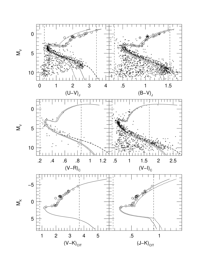
Figure 7: Photometry of stars in the Galactic open cluster M67 is compared to our 4 Gyr, solar-metallicity isochrone. Small crosses and large open circles represent photometry taken from Montgomery et al. (1993) and Houdashelt et al. (1992), respectively. The dotted line is the uncalibrated isochrone, while the solid line is the calibrated isochrone which is produced by applying the color calibrations given in Table 3 to the uncalibrated isochrone colors; the dashed-line portion of the isochrone results when the cool-dwarf color calibrations are used instead for the optical colors of the dwarf models having T_eff $<$ 5000 K. Vertical dashed lines show the color range of the field stars used to derive the color calibrations.

The (uncalibrated) colors of our 4 Gyr, solar-metallicity isochrone were determined by calculating synthetic spectra for effective temperature/surface gravity combinations lying along it, measuring synthetic colors from these spectra and then applying the Vega-based zero-point corrections to these colors. In Figure 7, we show the effects of applying the color calibrations to the synthetic colors of the 4 Gyr, Z_⊙ isochrone. In each panel of this figure, the uncalibrated isochrone is shown as a dotted line, while the calibrated isochrones are represented by a solid line (Table Improved Color–Temperature Relations and Bolometric Corrections for Cool Stars color calibrations throughout) and a dashed line (Table Improved Color–Temperature Relations and Bolometric Corrections for Cool Stars relations + cool-dwarf calibrations for optical colors of main-sequence stars cooler than 5000 K), respectively. The M67 UBVRI photometry of Montgomery et al. (1993) is shown as small crosses in Figure 7, and the giant-star data tabulated by Houdashelt et al. (1992) are represented by open circles.

We have corrected the M67 photometry for reddening using E(B–V) = 0.06 and the reddening ratios of a K star as prescribed by Cohen et al. (1981); we also assumed E(U–V)/E(B–V) = 1.71. This reddening value is on the upper end of the range of recent estimates for M67 (Janes & Smith (1984), Nissen et al. (1987), Hobbs & Thorburn (1991), Montgomery et al. (1993), Meynet et al. (1993), Fan et al. (1996)), but we found that a reddening this large produced the best overall agreement between the 4 Gyr, solar-metallicity isochrone and the M67 photometry in the region of the main-sequence turnoff for the complete set of CMDs which we examined. This reddening leaves the isochrone turnoff a bit bluer than the midpoint of the turnoff-star color distribution in V–I and a bit redder than the analogous M67 photometry in U–V, but it gives a reasonable fit for the other colors. Because the turnoff stars in the M_V, U–V CMD suggest a smaller reddening is more appropriate, we also examined the possibility that the Montgomery et al. (1993) V–I colors are systematically in error; however, they are consistent with the photometry of M67 reported by Chevalier & Ilovaisky (1991) and by Joner & Taylor (1990). Most importantly, we simply trust our synthetic V–I colors (and the corresponding reddening ratios) more than those in U–V, given the aforementioned uncertainties in the bound-free Fe I opacity, so we accepted the poorer turnoff fit in the U–V CMD. We derived the absolute magnitudes of the M67 stars, after correcting for extinction, assuming (m–M)₀ = 9.60 (Nissen et al. (1987), Montgomery et al. (1993), Meynet et al. (1993), Dinescu et al. (1995), Fan et al. (1996)).

The agreement between the isochrone and the M67 observations is improved in all of the CMDs (except perhaps in the H–K diagram, which is not shown) after the isochrone colors have been calibrated to the photometric systems using the color calibrations derived in Section 3.2.2. In fact, if we concentrate upon the main-sequence-turnoff region, there is no further indication of problems with the synthetic colors, with the possible exception of U–V, which again is sensitive to opacity uncertainties. The level of agreement between the photometry and the isochrone along the red-giant branch strengthens this conclusion. Of course, more R-band and deeper near-infrared photometry of M67 members would be helpful in verifying this result for the respective colors.

We also note that the detailed fit of the isochrone to the M67 turnoff could possibly be improved by including convective overshooting in our stellar interior models. While there is no general agreement regarding the importance of convective overshooting in M67 (see Demarque et al. (1992), Meynet et al. (1993), and Dinescu et al. (1995) for competing views), solar-metallicity turnoff stars only slightly more massive than those in M67 do show evidence for significant convective overshooting (Nordström et al. (1997), Rosvick & VandenBerg (1998)). To help us examine this further, VandenBerg (1999) has provided us with a 4 Gyr, solar-metallicity isochrone which includes the (small) amount of convective overshooting which he considers to be appropriate for M67. This isochrone is in excellent agreement with ours along the lower main-sequence but contains a “hook” feature at the main-sequence turnoff, becoming cooler than our 4 Gyr, Z_⊙ isochrone at M_V=3.5 and then hooking back to be hotter than ours at M_V=3.0; this “hook” does appear to fit the M67 photometry slightly better. Still, we do not expect convective overshooting to significantly affect our evolutionary synthesis models of elliptical galaxies because it will have an even smaller impact upon the isochrones older than 4 Gyr.

In those colors for which the deepest photometry is available, the calibrated isochrone is still bluer than the M67 stars on the lower main-sequence when only the color calibrations of Table Improved Color–Temperature Relations and Bolometric Corrections for Cool Stars are applied. Using separate calibrations for the cool dwarfs makes the faint part of the calibrated isochrone agree much better with the U–V and B–V colors of the faintest M67 stars seen in Figure 7 but appears to overcorrect their V–I colors. This improved fit between the calibrated isochrone and the M67 photometry supports the use of different color calibrations for the optical colors of the cool dwarfs, although there is a hint in Figure 7 that perhaps the cool-dwarf calibrations should apply at an effective temperature slightly hotter than 5000 K. Nevertheless, we do not find lower main-sequence discrepancies as worrisome as color differences near the turnoff would be, since the lowest-mass stellar interior models are sensitive to the assumed low-temperature opacities, equation of state and surface pressure boundary treatment. In addition, these faint, lower-main-sequence stars make only a small contribution to the integrated light of our evolutionary synthesis models when a Salpeter IMF is assumed. Consequently, small errors in their colors will not generally have a detectable effect on the integrated light of the stellar population represented by the entire isochrone.

3.3 Uncertainties in the Synthetic Colors

While the color calibrations are technically appropriate only for stars with near-solar metallicities, there is no evidence from the photometry of the field star sample that the synthetic color calibrations depend upon chemical composition. In fact, it is likely that we are at least partially accounting for metallicity effects by applying color corrections as a function of color rather than effective temperature. If the differences between the uncalibrated, synthetic colors and the photometry are due to errors in the synthetic spectra caused by missing opacity, for example, then different color corrections would be expected for two stars having the same temperature but different metallicities; the more metal-poor star should require a smaller correction. This is in qualitative agreement with the calibrations derived here, since this star would be bluer than its more metal-rich counterpart.

In this section, we present the sensitivities of the colors to uncertainties in some of the model parameters: effective temperature, surface gravity, metallicity, microturbulent velocity ($\xi$) and mixing. We estimate the uncertainties in these stellar properties to be $\pm$80 K in T_eff, $\pm$0.3 dex in log g, $\pm$0.25 dex in [Fe/H], and $\pm$0.25 km s^-1 in $\xi$. To examine the implications of these uncertainties, we have varied the model parameters of the coolest dwarf (61 Cyg B), the coolest giant ($\alpha$ Tau) and the hottest solar-metallicity dwarf (HR 4102) listed in Table Improved Color–Temperature Relations and Bolometric Corrections for Cool Stars by the estimated uncertainties, constructing new model atmospheres and synthetic spectra of these stars. We also constructed an $\alpha$ Tau model which neglected mixing. In Table Improved Color–Temperature Relations and Bolometric Corrections for Cool Stars, we present the changes in the uncalibrated synthetic colors which result when each of the model parameters is varied as described above. The color changes presented in this table are the average changes produced by parameter variations in the positive and negative directions. Since the VJHK color changes were almost always identical for colors on the Johnson-Glass and CIT/CTIO systems, the $\Delta$(V–K), $\Delta$(J–K) and $\Delta$(H–K) values given in Table Improved Color–Temperature Relations and Bolometric Corrections for Cool Stars are applicable to either system.

If our uncertainty estimates are realistic, then it is clear from Table Improved Color–Temperature Relations and Bolometric Corrections for Cool Stars that the variations in most colors are dominated by the uncertainties in one parameter. For the V–R, V–I, V–K, J–K and H–K colors, this parameter is T_eff, with the exception being the V–R color of the cool dwarf, which appears to be especially metallicity-sensitive. The behavior of the U–V and B–V colors is more complicated. Gravity and metallicity uncertainties dominate U–V for the cool giant and the hot dwarf, but effective temperature uncertainties have the greatest influence on the U–V color of the cool dwarf. Uncertainties in each of the model parameters have a similar significance in determining the B–V color of the cool giant, while those in T_eff dominate for the cool dwarf, and T_eff and [Fe/H] uncertainties are most important in the hot dwarf. Overall, we conclude that estimating the formal uncertainties of the synthetic colors needs to be done on a star-by-star and color-by-color basis, which we have not attempted to do. However, it is encouraging to see that T_eff uncertainties dominate so many of the color determinations, since our effective temperature scale is well-established by the angular diameter measurements discussed in Section 3.2.1.

4 The New Color-Temperature Relations and Bolometric Corrections

From the comparisons of the calibrated, 4 Gyr, solar-metallicity isochrone and the CMDs of M67, we conclude that the color calibrations that were derived in Section 3.2.2 and presented in Table Improved Color–Temperature Relations and Bolometric Corrections for Cool Stars generally put the synthetic colors onto the photometric systems of the observers but leave some of the optical colors of cool dwarfs too blue. These calibrations, coupled with the previously described improvements in the model atmospheres and synthetic spectra, have encouraged us to calculate a new grid of color-temperature relations and bolometric corrections. The bolometric corrections are calculated after calibrating the model colors, assuming BC_V,⊙ = –0.12 and M_V,⊙ = +4.84; when coupled with the calibrated color of our solar model, (V–K)_CIT = 1.530, we derive M_K,⊙ = +3.31 and BC_K,⊙ = +1.41. However, keep in mind that the color calibrations have been derived from Population I stars, so the colors of the models having [Fe/H] $\lesssim$ –0.5 should be used with some degree of caution (but see Section 3.3).

In Table Improved Color–Temperature Relations and Bolometric Corrections for Cool Stars, we present a grid of calibrated colors and K-band bolometric corrections for stars having 4000 K $\leq$ T_eff $\leq$ 6500 K and 0.0 $\leq$ log g $\leq$ 4.5 at five metallicities between [Fe/H] = –3.0 and solar metallicity; the optical colors of the dwarf (log g = 4.5) models resulting from the use of the cool-dwarf color calibrations discussed in Section 3.2.2 are enclosed in parentheses, allowing the reader to decide which color calibrations to adopt for these models. We will now proceed to compare our new, theoretical color-temperature relations to empirical relations of field stars and to previous MARCS/SSG results.

4.1 Comparing Our Results to Other Empirical Color-Temperature Relations

In the following sections, we use the photometry and effective temperatures of the stars listed in Table Improved Color–Temperature Relations and Bolometric Corrections for Cool Stars to derive empirical color-temperature relations for field giants and field dwarfs. We then compare our models and our empirical, solar-metallicity color-temperature relations to the CT relations of field stars which have been derived by Blackwell & Lynas-Gray (1994; hereafter BLG (94)), Gratton et al. (1996; hereafter GCC (96)), Bessell (1979; hereafter B (79)), Bessell (1995; hereafter B (95)), Bessell et al. (1998; hereafter BCP (98)) and Bessell (1998; hereafter B (98)).

4.1.1 The Color-Temperature Relations of Our Field Stars

The color and temperature data for our set of color-calibrating field stars are plotted in Figures 8 and 9, where we have split the sample into giants (log g $\leq$ 3.6) and dwarfs (log g $>$ 3.6), shown in the lower and upper panels of the figures, respectively. We have fit quadratic relations to the effective temperatures of the dwarfs and giants separately as a function of color to derive empirical, solar-metallicity color-temperature relations for each; the resulting CT relations of the giants and dwarfs are shown as bold, solid lines and bold, dotted lines, respectively, in these figures. The coefficients of the fits (and their 1$\sigma$ uncertainties) are given in Table Improved Color–Temperature Relations and Bolometric Corrections for Cool Stars. The calibrated colors of our M67 isochrone (4 Gyr, Z_⊙) are also plotted in Figures 8 and 9 as solid lines; the dashed lines in the upper panels of Figure 8 show the calibrated isochrone when the cool-dwarf color calibrations are applied. Comparisons with our other isochrones indicate that the CT relation of the solar-metallicity isochrones is not sensitive to age.

Although we have divided our field-star sample into giants and dwarfs, the empirical CT relations of the two groups only appear to differ significantly in (V–R)_C and (V–I)_C. In B–V and J–K, the CT relations of the dwarfs and giants are virtually identical, and it is only the color of the coolest dwarf that prevents the same from being true in V–K. The differences in the U–V color-temperature relations of the dwarfs and giants can largely be attributed to the manner in which we chose to perform the least-squares fitting. Therefore, we want to emphasize that our tabulation of separate CT relations for dwarfs and giants does not necessarily infer that the two have significantly different colors at a given T_eff.

It is apparent that the calibrated isochrone matches the properties of the field giants very nicely in Figures 8 and 9 and, in fact, is usually indistinguishable from the empirical CT relation. However, using the color calibrations of Table Improved Color–Temperature Relations and Bolometric Corrections for Cool Stars, the dwarf and giant portions of the isochrone diverge cooler than $\sim$5000 K in all colors; this same behavior is not always seen in the stellar data. This discrepancy at cool temperatures means that one of the following conditions must apply: 1) the field star effective temperatures of the cool dwarfs are systematically too hot; 2) the isochrones predict the wrong T_eff/gravity relation for cool dwarfs; or 3) the cool dwarf temperatures and gravities are correct but the model atmosphere and/or synthetic spectrum calculations are wrong for these stars. Only the latter condition would lead to different color calibrations being required to put the colors of cool dwarfs and cool giants onto the photometric systems.

The previously-mentioned comparison between our isochrones and those of VandenBerg (1999) lead us to believe that the lower main-sequence of our 4 Gyr, solar-metallicity isochrone is essentially correct, so it would appear that the synthetic colors of the coolest dwarf models are bluer than the color calibrations of Table Improved Color–Temperature Relations and Bolometric Corrections for Cool Stars would predict because either we have adopted incorrect effective temperatures for these stars or there is some error in the model atmosphere or synthetic spectrum calculations, such as a missing opacity source.

Unpublished work on CO band strengths in cool dwarfs suggests that part of the problem could lie with the BG89 temperatures derived for these stars. In addition, some IRFM work (Alonso et al. 1996) indicates that the effective temperatures adopted for our K dwarfs cooler than 5200 K may be too hot by $\sim$100 K and infers an even larger discrepancy (up to 400 K) for HR 8086. A recent angular diameter measurement (Pauls (1999)) also predicts a hotter T_eff than we adopted for HR 1084. If our K-dwarf effective temperatures are too warm, this would imply that the cool-dwarf color calibrations should not be used because the errors lie in the model parameters adopted for the cool dwarfs and not in the calculation of their synthetic spectra. However, T_eff errors of 100 K are not sufficiently large to make the three cool field dwarfs lie on the optical color calibrations of the other stars (see Table Improved Color–Temperature Relations and Bolometric Corrections for Cool Stars). In addition, the similarities of the V–K and J–K colors of our two coolest dwarfs and those of the calibrated isochrone at the assumed effective temperatures argue that the T_eff estimates are essentially correct but do not preclude temperature changes of the magnitude implied by the IRFM and angular diameter measurements. Thus, some combination of T_eff errors and model uncertainties may conspire to produce the color effects seen here, and more angular diameter measurements of K dwarfs would be very helpful in sorting out these possibilities. Nevertheless, the use of the cool-dwarf color calibrations improves the agreement between the models and the empirical data so remarkably well in Figures 7 and 8 that a good case can be made for their adoption.

As discussed in the Section 3.3, the model B–V colors of giants are noticeably dependent on gravity at low temperatures. The agreement between the observed B–V colors and the corresponding calibrated, synthetic colors for both the sample of field stars and the cool M67 giants suggests that the gravity-temperature relation of the isochrone truly represents the field stars, even at cool temperatures. While this is certainly anticipated, the fact that it occurs indicates that the surface boundary conditions and mixing-length ratio used for the interior models are satisfactory and gives us confidence that these newly-constructed isochrones are reasonable descriptions of the stellar populations they are meant to represent in our evolutionary synthesis program.

4.1.2 Other Field-Star Color-Temperature Relations

BLG (94) estimated effective temperatures for 80 stars using the IRFM and derived V–K, T_eff relations for the single stars, known binaries and total sample which they studied. Because these three relations are very similar, we have adopted their single star result for our comparisons, after converting their V–K colors from the Johnson to the Johnson-Glass system using the color transformation given by Bessell & Brett (1988). We expect the BLG (94) effective temperature scale to be in good agreement with that adopted here for the field stars used to derive the color calibrations – for the 19 stars in common between BLG (94) and BG (89), BLG (94) report that the average difference in T_eff is 0.02%. For later discussion, we note that the coolest dwarf included in BLG (94)’s sample is BS 1325, a K1 star, with T_eff = 5163 K.

GCC (96) derived their CT relations from photometry of about 140 of the BG (89) and BLG (94) stars. They adjusted BG (89)’s IRFM T_eff estimates to put them onto the BLG (94) scale and then fit polynomials to the effective temperatures as a function of color to determine CT relations in Johnson’s B–V, V–R, R–I, V–K and J–K colors. In each color, they derived three relations – one represents the dwarfs, and the other two apply to giants bluer and redder than some specific color. For these relations, we have used B (79)’s color transformations to convert the Johnson V–R and V–I colors to the Cousins system; Bessell & Brett (1988) again supplied the V–K and J–K transformations to the Johnson-Glass system.

BCP (98) combined the IRFM effective temperatures of BLG (94) and temperatures estimated from the angular diameter measurements of di Benedetto & Rabbia (1987), Dyck et al. (1996) and Perrin et al. (1998) to derive a polynomial relation between V–K and T_eff for giants. The color-temperature relations provided by B (98) are presumably derived in exactly the same manner from this same group of stars. For cool dwarfs, BCP (98) also determined a CT relation, this time in V–I, from the IRFM effective temperatures of BLG (94) and Alonso et al. (1996).

B (79) merged his V–I, V–K color-color relation for field giants and the V–K, T_eff relation of Ridgway et al. (1980) to come up with a V–I, T_eff relation. He then combined this with V–I, color trends to define CT relations for giants in other colors. By assuming that the same V–I, T_eff relation applied to giants and dwarfs with 4000 K $\leq$ T_eff $\leq$ 6000 K, B (79) derived dwarf-star CT relations in a similar manner. For the coolest dwarfs, updated versions of B (79)’s V–R, T_eff and V–I, T_eff relations were given by B (95).

4.1.3 Comparisons of the Color-Temperature Relations

We compare our calibrated, solar-metallicity color grid to empirical determinations of color-temperature relations of field stars in Figures 10–14. For these comparisons, we break our grid up into giants & subgiants, which we equate with models having 0.0 $\leq$ log g $\leq$ 4.0, and dwarfs (log g = 4.5). In all of the figures in this section, the giant-star CT relations appear in the upper panels, and the lower panels give the dwarf relations. The calibrated colors of our solar-metallicity grid are shown as open circles (or as asterisks when the cool-dwarf color calibrations have been used), but to relieve crowding in the giant-star plots, we connect the model colors at a given T_eff by a solid line and plot only the highest and lowest gravity models as open circles. Our empirical color-temperature relations (Table Improved Color–Temperature Relations and Bolometric Corrections for Cool Stars) are shown as solid lines in Figures 10–14; the CT relations taken from the literature are represented by the symbols indicated in the figures. In addition, our calibrated, solar-metallicity, 4 Gyr isochrone is shown as a dotted line; the dashed line in the dwarf-star panels of Figures 10–12 is the calibrated isochrone which results when the cool-dwarf color calibrations have been used. Comparisons with our other solar-metallicity isochrones shows that this CT relation is insensitive to age, so it should agree closely with the field-star relations. We omit the U–V and H–K color-temperature relations from these comparisons because we are not aware of any recent determinations of field-star relations in these colors, which nevertheless are less well-calibrated than the others.

For the giant stars, our empirical CT relations are in excellent agreement with the field relations of BLG (94), GCC (96), BCP (98) and B (98), with the temperature differences at a given color usually much less than 100 K. The 4 Gyr, Z_⊙ isochrone also matches the field-giant relations quite well, as would be expected from Figures 8 and 9. In fact, most of the (small) differences between our empirical CT relations and the isochrone are probably due to our decision to use quadratic relations to represent the field stars; a quadratic function may not be a good representation of the true color-temperature relationships, and such a fit often introduces a bit of excess curvature at the color extremes of the observational data. The B (79) color-temperature relations for giants are also seen to be in good agreement with the other empirical and theoretical, giant-star data in V–R and V–I, but his B–V, T_eff relation is bluer than the others; we have not attempted to determine the reason for this discrepancy.

Overall, since the colors of the field giants lie within the bounds of our solar-metallicity grid at a given effective temperature and also show good agreement with the 4 Gyr isochrone, our calibrated models are accurately reproducing the colors of solar-metallicity, F–K field giants of a specific temperature and surface gravity. Unfortunately, the dwarf-star color-temperature relations do not show the same level of agreement as those of the giants, overlying one another for T_eff $\gtrsim$ 5000 K but diverging at cooler effective temperatures. Therefore, we will examine each of the CT relations of the dwarfs individually.

In B–V (Figure 10), the field stars from Table Improved Color–Temperature Relations and Bolometric Corrections for Cool Stars produce a CT relation which is in good agreement with that of GCC (96). When using the color calibrations of Table Improved Color–Temperature Relations and Bolometric Corrections for Cool Stars, our isochrone and grid models of cool dwarfs are bluer than the empirical relations at a given T_eff, which is consistent with the comparison to M67 in Figure 7, indicating that these calibrated B–V colors are too blue. On the other hand, the agreement between these models and the CT relation of B (79) suggests that these grid and isochrone colors are essentially correct. Similar quandaries are posed by the color-temperature relations of the dwarfs in V–R and V–I (Figures 11 and 12). Here, the B (79) relations predict slightly bluer colors than the analogous isochrone and grid models at a given temperature, but B (95)’s updated data for the coolest dwarfs agrees with our calibrated isochrone and models quite well. Our empirical CT relations for dwarfs and the GCC (96) data, on the other hand, lie to the red of these models and isochrones, again showing the same kind of discrepancy seen in the M67 comparisons. Unfortunately, the BCP (98) V–I, T_eff relation does not extend to cool enough temperatures to help resolve the situation. Supplementing the color calibrations of Table Improved Color–Temperature Relations and Bolometric Corrections for Cool Stars with the (optical) cool-dwarf color calibrations, however, brings the solar-metallicity isochrone and models into agreement with all of the field-dwarf CT relations of GCC (96) instead.

In Figure 13, we also see that there is one empirical CT relation (BLG (94)) which indicates that our cool-dwarf models are essentially correct at a given T_eff, while another (GCC (96)) predicts that they are too blue, although the magnitude of disagreement in this figure is much smaller than that seen in Figures 10–12. Since we are not aware of any near-infrared photometry for lower-main-sequence stars in M67, we cannot use Figure 7 to bolster any of the V–K CT relations. The only color in which all of the theoretical and empirical data are in relative agreement for the dwarfs is J–K; this is shown in Figure 14.

We hesitate to emphasize the similarities between our empirical color-temperature relations and the others plotted in the dwarf-star panels of Figures 10–14. Our V–K CT relation for field stars only differs from that of BLG (94) because they neglected to treat dwarfs and giants separately; if we do the same, these differences disappear. Even so, the coolest dwarf in the BLG (94) study was BS 1325, a K1 V star with T_eff = 5163 K, which is hotter than the temperature at which the dwarf and giant CT relations begin to bifurcate, so it is somewhat misleading to extend BLG (94)’s relation to redder colors in the dwarf-star panel of Figure 13. Likewise, it is not surprising that our CT relations and GCC (96)’s relations are so compatible – GCC (96) used the BLG (94) and BG (89) data to define their relations, so the cool end of their dwarf relations are defined by the same cool dwarfs included in our sample. The poor agreement between the other empirical CT relations and the dwarf-star relations of B (79) is probably due to the manner in which B (79) derived his field-star relations. He assumed a similar V–I, T_eff relation for cool dwarfs and cool giants, an assumption which Figure 8 suggests to be inappropriate.

Overall, then, if we assume that the effective temperatures and photometry that we have adopted for the field stars of Table Improved Color–Temperature Relations and Bolometric Corrections for Cool Stars and the members of M67 are all correct, we can account for the similarities and the differences between our color-temperature relations and those taken from the literature. In this case, it appears that the CT relations of GCC (96) are the most representative of field dwarfs, while each of those which we have examined are probably equally reliable for the field giants (except B (79)’s B–V, T_eff relation). This also produces a consistent picture in which both the field-star CT relations and the M67 photometry indicate that our model colors for cool dwarfs are too blue at a given effective temperature if only the color calibrations of Table Improved Color–Temperature Relations and Bolometric Corrections for Cool Stars are employed; adopting the cool-dwarf color calibrations for T_eff $<$ 5000 K then brings the models and the observational data into close agreement.

However, we can envision an alternate scenario in which the coolest three (or more) field dwarfs have been assigned effective temperatures which are too hot. By lowering T_eff by $\sim$100 K for HR 8085 and HR 8832 and by $\sim$200 K for HR 8086, these stars would lie along the the same color calibrations as the other field stars in all colors except perhaps U–V and B–V. This would shift our empirical CT relations and those of GCC (96) to bluer colors for the cool dwarfs and thus resolve the disagreement with B (95)’s relations and the models calibrated using the Table Improved Color–Temperature Relations and Bolometric Corrections for Cool Stars color calibrations. It would also leave V–R and V–I as the only two colors in which the dwarf-star and giant-star CT relations differ significantly, which is understandable, since the V, R and I bands contain many molecular features (e.g., TiO, CN) which are gravity-sensitive. However, the discrepancies between the calibrated, 4 Gyr, solar-metallicity isochrone (solid line in Figure 7) and the U–V and B–V photometry of the lower main-sequence of M67 would likely remain.

Since it is not clear to us which of these situations applies, we have presented the calibrated model colors for each case here. The essential pieces of information needed to disentangle these two possibilities are angular diameter measurements of K dwarfs; these would certainly aid us in testing the BG (89) temperatures of the cool dwarfs in our sample and confirming their CT relations. However, for the time-being, the small number of cool dwarfs with effective temperature estimates and the fact that such stars make only a small contribution to the integrated light of a galaxy have led us to adopt the calibration relations given in Table Improved Color–Temperature Relations and Bolometric Corrections for Cool Stars for the synthetic colors of all of our evolutionary synthesis models.

4.2 Comparisons to Previous MARCS/SSG Color-Temperature Relations

In Figures 15 and 16, we compare our new, solar-metallicity CT relations to the previous MARCS/SSG results published by VB (85) and BG (89); the models of the former and latter are shown as open and filled circles, respectively. In each panel of these figures, we plot log g vs. color and use dotted lines to represent isotherms resulting from the uncalibrated colors of our models; the isotherms produced by our improved, calibrated colors (Table Improved Color–Temperature Relations and Bolometric Corrections for Cool Stars calibrations only) are shown as solid lines. Thus, differences between the older colors and the appropriate dotted line can be identified with improvements in the models and color measurements, and differences between the dotted and solid lines of the same temperature can be equated with the effects of calibrating the synthetic colors.

4.2.1 The Optical Color-Temperature Relations

In the upper panel of Figure 15, we compare our CT relations and the B–V colors calculated by VB (85) using the filter-transmission-profiles of Matthews & Sandage (1963). The calibrated B–V colors are always redder than their previous counterparts, but the uncalibrated colors of the new models do not differ appreciably from those of VB (85) for T_eff $\gtrsim$ 5000 K; the main improvement in the B–V colors of these hotter stars is due to the color calibrations. At 4500 K, especially as log g decreases, the improved low-temperature opacity data used here becomes important, and this becomes the dominant improvement for cooler stars, although the color corrections inferred from the calibrations are still substantial.

The V–R colors of VB (85) and BG (89), measured with the R-band filter of Cousins (1980), are compared to our new, solar-metallicity color grid in the middle panel of Figure 15. Surprisingly, for effective temperatures hotter than about 5000 K, the colors of the older models are in good agreement with those of the newer, calibrated models; either the color differences produced by the filter-transmission-profiles adopted by each group are being almost exactly offset by the effects of the color calibrations which we have derived, or the newer opacities used here have moved the V–R colors of the models to the blue. For the cool giants, however, the calibrated V–R colors are significantly redder than those previously published.

For V–I, the new and old models are shown in the lower panel of Figure 15. This diagram is similar to the V–R plot in that it is difficult to disentangle the color changes produced by the use of different filter profiles (VB (85) and BG (89) use the I-band filter of Cousins 1980) and those resulting from improvements in the stellar modelling. It is apparent, however, that the previous MARCS/SSG V–I colors are too red at hotter temperatures (T_eff $\gtrsim$ 5500 K) and too blue at cooler temperatures.

4.2.2 The Near-Infrared Color-Temperature Relations

Figure 16 (upper panel) shows that the synthetic V–K colors on the CIT/CTIO system are not altered appreciably by calibration, at least with respect to the color range of the models and the magnitude of the color differences which exist between the newer and older models. While the colors of our models and those of BG (89) are about the same at T_eff = 4500 K, the newer models are redder at temperatures cooler than this and the older models are redder at hotter temperatures. Differences in the model atmospheres and synthetic spectra are responsible for these effects, since BG (89) used the same filter-transmission-profiles that we have.

The CIT/CTIO J–K colors shown in the lower panel of Figure 16 are all significantly bluer than those previously published. For the hotter models, improvements in MARCS and the much better treatment of line absorption in SSG are the major causes of these blueward shifts. In fact, the magnitude of the color differences between the older colors and the newer, uncalibrated colors is about the same at all temperatures. The color calibrations, however, while also making the model J–K colors bluer, grow in importance as T_eff decreases; this effect begins to dominate the color shifts due to the model improvements at T_eff $\sim$ 4500 K.

5 Conclusion

We have calculated colors and bolometric corrections for grids of stellar models having 4000 $\leq$ T_eff $\leq$ 6500 K, 0.0 $\leq$ log g $\leq$ 4.5 and –3.0 $\leq$ [Fe/H] $\leq$ 0.0. The synthetic colors which we measure include Johnson U–V and B–V; Cousins V–R and V–I; Johnson-Glass V–K, J–K and H–K; and CIT/CTIO V–K, J–K, H–K and CO. These synthetic colors have been determined by convolving the most recent estimates of the filter-transmission-profiles of the respective photometric systems with newly-calculated synthetic spectra. The synthetic spectra are produced by the SSG spectral synthesis code, which has been updated significantly, especially in terms of its low-temperature opacity data and spectral line lists. The MARCS model atmospheres which are used by SSG have also been calculated using this new opacity data and improved opacity distribution functions.

We have found that the initial synthetic colors require small corrections to be put onto the observational systems. Here, we have assembled a set of field stars which have effective temperatures measured using the infrared-flux method (IRFM), and we have used photometry of these stars to derive the color calibrations needed to put the synthetic colors onto the photometric systems. The scale factors and zero points of these calibrations are gratifyingly close to unity and small, respectively, but the UBVRI colors of the coolest dwarfs (T_eff $<$ 5000 K) may require a more substantial correction. Nevertheless, the specific color calibrations which we adopt are only applicable to models calculated with our versions of the MARCS and SSG computer codes. We encourage others to examine the need for such calibrations in their models as well.

Using the field-star data adopted in deriving the color calibrations, we have also found that the recent angular diameter measurements of Mozurkewich et al. (1991), Mozurkewich (1997) and Pauls et al. (1997) match the angular diameters predicted by Bell & Gustafsson (1989) very well, thus giving strong confirmation of the latter’s effective temperature scale, which we have adopted. Since most of the synthetic colors are much more sensitive to effective temperature than they are to the other model parameters, such as metallicity and surface gravity, this infers that the differences between the uncalibrated, synthetic colors and the field-star photometry are not caused by errors in the temperatures of the field-star models. The coolest field dwarfs may again prove an exception to this generalization, as none of their angular diameters have been measured and their effective temperatures are therefore more uncertain. Knowing that the IRFM-derived temperatures are accurate has also allowed us to determine empirical, color-temperature (CT) relations for these field F–K stars.

After calibrating our synthetic colors, our newly-calculated, 4 Gyr, Z_⊙ isochrone is seen to be in good agreement with optical and near-infrared color-magnitude diagrams of M67 from the upper main-sequence through the tip of the red-giant branch. For giants and for dwarfs hotter than about 5000 K, our theoretical, solar-metallicity CT relations and solar-metallicity isochrones are also found to match the empirical, field-star color-temperature relations derived here and found elsewhere in the literature. For the coolest dwarfs (T_eff $<$ 5000 K), there are some differences between our empirical color-temperature relations and the best-determined relations of others. The calibrated colors of the cool-dwarf models also remain a bit bluer than the field-star relations (at a given T_eff) and the M67 main-sequence stars (at a given absolute magnitude). Because we have not been able to determine whether the synthetic, optical colors of the cool dwarf models are too blue because their adopted effective temperatures are too hot or the synthetic spectra are in error, we present alternate UBVRI colors for our models having T_eff $<$ 5000 K and log g = 4.5. These colors are based upon separate color calibrations derived from only the cool field dwarfs and which greatly improve the agreement between the calibrated, synthetic colors and the empirical data. We leave it to the reader to decide which model colors they prefer.

This work would greatly benefit from further effective temperature estimates of cool dwarfs and measurements of the corresponding angular diameters needed to confirm them. It would also be quite useful to acquire additional photometry of the field stars used here to derive the color calibrations. Only a small subset of these stars, which includes no cool dwarfs, has been observed on the Cousins system, making the V–R and V–I color calibrations less well-determined than some of the others. In addition, only Johnson near-infrared photometry was available for the field stars. Color transformations had to be applied to this photometry before the Johnson-Glass and CIT/CTIO color calibrations could be derived; this also prohibited the determination of a similar calibration for the CIT/CTIO CO index.

Overall, the agreement between our theoretical CT relations and the empirical data and between our 4 Gyr, solar-metallicity isochrone and the photometry of M67 indicates that our synthetic spectra are generally providing a good representation of the spectral energy distributions of stars of the corresponding T_eff, surface gravity and metallicity. This conclusion is further supported by our synthetic spectra of M giants, which are presented in a companion paper (Houdashelt et al. 2000). In a future paper (Houdashelt et al. 2001), we will use similar synthetic spectra and newly-constructed isochrones as part of a program to simulate the spectral energy distributions of early-type galaxies through evolutionary synthesis.

Figure 1: Comparison of our synthetic spectra of the Sun and Arcturus ($\alpha$ Boo) and the observed spectra of these stars near the bandhead of the ¹²CO(4,2) band. Our synthetic spectra are shown as dotted lines in each panel. The observational data is shown as solid lines and has been taken from Farmer & Norton (1989) for the Sun (upper panel) and from Hinkle et al. (1995) for Arcturus (lower panel). The latter is ground-based, and the solid line along the lower part of the lower panel is the (substantial) amount of telluric absorption in this part of the spectrum (Hinkle et al. 1995); it is drawn in emission and to half-scale.

Figure 2: Comparison of our synthetic spectra of the Sun and Arcturus ($\alpha$ Boo) and the observed spectra of these stars near the center of the H band. Our synthetic spectra are shown as dotted lines in each panel. The observational data is shown as solid lines and has been taken from Livingston & Wallace (1991) for the Sun (upper panel) and from Hinkle et al. (1995) for Arcturus (lower panel). The solid lines along the lower part of each panel are the telluric absorption in this part of the spectrum; it is taken from the same sources as the empirical data and is drawn in emission and to half-scale.

Figure 3: The filter-transmission-profiles used to measure the synthetic colors are shown atop our synthetic spectrum of Arcturus (convolved to 2 Å resolution). The UBVR_CI_C filter profiles are those of Bessell (1990). We display only one of Bessell’s two B filter profiles, that which is used in the B–V calculations; it differs slightly from his BX filter used for U–B colors. The Johnson-Glass (JG) JHK filters are taken from Bessell & Brett (1988) and shown as dotted profiles in the lower panel of the figure. Persson (1980) and Frogel et al. (1978) supplied the JHK and CO filter profiles of the CIT/CTIO system, respectively. These are shown as solid lines in the lower panel, and the continuum filter used for the CO index is labeled “cont.”

Figure 4: Comparison of the angular diameters measured by Mozurkewich et al. (1991) and Mozurkewich (1997; M97 collectively) and those estimated from the “adopted” effective temperatures of Bell & Gustafsson (1989; BG89). All angular diameters are limb-darkened values; the M97 data plotted here were derived from his uniform-disk diameters as described in the text. Error bars are those reported by the original authors; the M97 uncertainties are approximately the size of the symbols in the upper panel. Measurements for G–K supergiants and giants are shown as open circles and open triangles, respectively; subgiants are shown as open squares. The upper panel presents the angular diameter comparison, and the solid line represents equality of the BG89 and M97 diameters. The lower panel shows the absolute differences in the angular diameter estimates of the individual stars.

Figure 5: The field stars used to calibrate the synthetic colors are plotted in the H-R diagram. The solid lines in each panel are our 3 Gyr and 16 Gyr, solar-metallicity isochrones. The six panels show a) the entire sample of stars, b) those having [Fe/H] $<$ –0.3, c) the stars with [Fe/H] $>$ +0.2, d) the solar-metallicity (–0.3 $\leq$ [Fe/H] $\leq$ +0.2) dwarfs and subgiants (classes IV and V), e) the solar-metallicity normal giants (class III), and f) the solar-metallicity bright giants (classes I and II). The three stars which lie in unexpected positions in the H-R diagram are shown as filled points and are discussed in the text – they are $\gamma$ Tuc, a metal-poor star with T_eff = 6530 K; 72 Cyg, a metal-rich, 4715 K giant; and 31 Com, a (peculiar) solar-metallicity giant having T_eff = 5761 K.

Figure 6: Some of the color calibrations required to put the synthetic colors onto the observational systems are illustrated. Solid lines are the linear, least-squares fits to the data, excluding the three coolest dwarfs; dashed lines are the cool-dwarf color calibrations described in the text. Dotted lines show equality of the synthetic and photometric colors. Filled symbols represent dwarfs and subgiants (luminosity classes IV, V), and open symbols are giants and supergiants (luminosity classes I, II, III). Sources of the photometry are described in the text and listed in Table 2.

Figure 8: The empirical, optical color-temperature relations of our sample of field dwarfs (upper panels) and field giants (lower panels) are shown. The bold, solid and bold, dotted lines are quadratic fits to the field-giant and field-dwarf data, respectively; the coefficients of these relations are given in Table 6. The solid line is our calibrated, 4 Gyr, Z_⊙ isochrone (using the color calibrations of Table 3); the dashed line results when the cool-dwarf color calibrations are used instead for the optical colors of the dwarf models having T_eff $<$ 5000 K.

Figure 9: The empirical, near-infrared color-temperature relations of our sample of field dwarfs (upper panels) and field giants (lower panels) are shown. The bold, solid and bold-dotted lines are quadratic fits to the field-giant and field-dwarf data, respectively; the coefficients of these relations are given in Table 6. The solid line is our calibrated, 4 Gyr, Z_⊙ isochrone.

Figure 10: The Johnson B–V colors of the solar-metallicity models are compared to (B–V) vs. effective temperature relations of field stars. The upper panel presents the comparison for giants; the lower panel shows dwarfs. In both panels, our model colors (HBS) are shown as open circles (connected by solid lines in the giant-star panels), and the dotted lines are the color-temperature relations predicted by our 4 Gyr, Z_⊙ isochrone when the color calibrations of Table 3 are used; the dashed line and asterisks are the lower main-sequence of the calibrated isochrone and the HBS models, respectively, when the cool-dwarf color calibrations are used instead for the dwarf models having T_eff $<$ 5000 K. The solid lines are the empirical relations derived here from the photometry of the field stars used to calibrate the synthetic colors. The field relations of Gratton et al. (1996; GCC96), Bessell (1979; B79) and Bessell (1998; B98) are represented by open triangles, filled squares and open squares, respectively.

Figure 11: The Cousins V–R colors of the solar-metallicity models are compared to (V–R) vs. effective temperature relations of field stars. The upper panel presents the comparison for giants; the lower panel shows dwarfs. In both panels, our model colors (HBS) are shown as open circles (connected by solid lines in the giant-star panels), and the dotted lines are the color-temperature relations predicted by our 4 Gyr, Z_⊙ isochrone when the color calibrations of Table 3 are used; the dashed line and asterisks are the lower main-sequence of the calibrated isochrone and the HBS models, respectively, when the cool-dwarf color calibrations are used instead for the dwarf models having T_eff $<$ 5000 K. The solid lines are the empirical relations derived here from the photometry of the field stars used to calibrate the synthetic colors. The field relations of Gratton et al. (1996; GCC96), Bessell (1979; B79), Bessell (1998; B98) and Bessell (1995; B95) are represented by open triangles, filled squares, open squares and crosses, respectively.

Figure 12: The Cousins V–I colors of the solar-metallicity models are compared to (V–I) vs. effective temperature relations of field stars. The upper panel presents the comparison for giants; the lower panel shows dwarfs. In both panels, our model colors (HBS) are shown as open circles (connected by solid lines in the giant-star panels), and the dotted lines are the color-temperature relations predicted by our 4 Gyr, Z_⊙ isochrone when the color calibrations of Table 3 are used; the dashed line and asterisks are the lower main-sequence of the calibrated isochrone and the HBS models, respectively, when the cool-dwarf color calibrations are used instead for the dwarf models having T_eff $<$ 5000 K. The solid lines are the empirical relations derived here from the photometry of the field stars used to calibrate the synthetic colors. The field relations of Gratton et al. (1996; GCC96), Bessell (1979; B79), Bessell (1998; B98), Bessell et al. (1998; BCP98) and Bessell (1995; B95) are represented by open triangles, filled squares, open squares (giants), open squares (dwarfs) and crosses, respectively.

Figure 13: The Johnson-Glass V–K colors of the solar-metallicity models are compared to (V–K) vs. effective temperature relations of field stars. The upper panel presents the comparison for giants; the lower panel shows dwarfs. In both panels, our model colors (HBS) are shown as open circles (connected by solid lines in the giant-star panels), and the dotted lines are the color-temperature relations predicted by our 4 Gyr, Z_⊙ isochrone. The solid lines are the empirical relations derived here from the photometry of the field stars used to calibrate the synthetic colors. The field relations of Gratton et al. (1996; GCC96), Bessell et al. (1998; BCP98) and Blackwell & Lynas-Gray (1994; BLG94) are represented by open triangles, open squares and filled squares, respectively.

Figure 14: The Johnson-Glass J–K colors of the solar-metallicity models are compared to (J–K) vs. effective temperature relations of field stars. The upper panel presents the comparison for giants; the lower panel shows dwarfs. In both panels, our model colors (HBS) are shown as open circles (connected by solid lines in the giant-star panels), and the dotted lines are the color-temperature relations predicted by our 4 Gyr, Z_⊙ isochrone. The solid lines are the empirical relations derived here from the photometry of the field stars used to calibrate the synthetic colors. The field relations of Gratton et al. (1996; GCC96) are represented by open triangles.

Figure 15: The Johnson B–V, Cousins V–R and Cousins V–I colors of the current and previously-published MARCS/SSG models are compared in the upper, middle and lower panels, respectively. The uncalibrated colors of our solar-metallicity models of a given effective temperature are shown as dotted lines; solid lines give the corresponding calibrated colors. Each set of models is labeled with the T_eff of the isotherm. Colors taken from Bell & Gustafsson (1989; BG89) are shown as filled circles and those of VandenBerg & Bell (1985; VB85) as open circles.

Figure 16: The CIT/CTIO V–K and J–K colors of the current and previously-published MARCS/SSG models are compared in the upper and lower panels, respectively. The uncalibrated colors of our solar-metallicity models of a given effective temperature are shown as dotted lines; solid lines give the corresponding calibrated colors. Each set of models is labeled with the T_eff of the isotherm. Colors taken from Bell & Gustafsson (1989) are shown as filled circles.

References

- (1) Alonso, A., Arribas, S., & Martínez-Roger, C. 1996, A&AS, 117, 227
- Ažusienis & Straižys (1969) Ažusienis, A., & Straižys, V. 1969, Soviet Astron. J., 13, 316