Simultaneous intensive photometry and high resolution spectroscopy of $\delta$ Scuti stars IV. An improved picture of the pulsational behaviour of X Caeli.

Abstract

The $\delta$ Scuti star X Caeli has been the target of a simultaneous photometric (14 consecutive nights) and spectroscopic campaign (8 consecutive nigths). From the analysis of light curves we were able to pick up 17 frequency components, most of which were already detected in two previous campaigns. The comparison with the results of the previous campaigns shows that while some terms are rather stable (in particular the dominant mode at 7.39 cd^-1 ) others have conspicuous amplitude variations. 14 photometric terms have been also detected in the radial velocity curve or in the analysis of the line profile variations. There are no spectroscopic terms without photometric counterparts, and this means that there are no high–degree modes as observed in other $\delta$ Scuti stars. The simultaneous fit of light and line profile variations has allowed the estimation of the inclination of rotational axis (about $70^{o}$) and the $\ell,m$ identification for many modes. In particular there is clear evidence that the two shortest period modes are retrograde. Rather reliable results were found for the dominant mode which has $\ell=1$, $m=-1$. The resulting physical parameters of its pulsation are in good agreement with the prediction of theoretical models and suggest for this star a mixing length parameter of about 0.5. Finally the fundamental stellar physical parameters and their refinement are discussed in the light of the identification of the 7.47 cd^-1   term as a radial mode.

1 Introduction

X Cae has been recently the target of two campaigns: the first photometric in 1989 (Mantegazza & Poretti, 1992, Paper I) and the second both photometric and spectroscopic in 1992 (Mantegazza & Poretti 1996, Paper II).

From the photometric data obtained in these campaigns it has been possible to single out 14 terms due to at least 6 independent pulsation modes and to some harmonics and non–linear couplings among the strongest ones. With the additional information supplied by the high resolution spectroscopy, an attempt has been performed to identify at least some of these modes. However, due to the rather short baseline of spectroscopic data (4 consecutive nights), only very preliminary results have been obtained. The only really confident result was that the dominant mode (7.39 cd^-1 ) has $m=-1$ and $\ell=$ 1 or 2. A successive improved analysis of these data (Mantegazza & Poretti, 1998) favoured the choice of $\ell=1$ and $m=-1$, and suggested that the rotational axis inclination is larger than $45^{o}$. About the other modes the conclusion was that they are probably non-radial with $\ell=2\pm 1$, while high–degree sectorial modes, which seem to be rather common in fast rotating $\delta$ Scuti stars (Mantegazza, 1997; Kennelly et al., 1998), were not observed. The comparison between the photometric data of the two campaigns shows that while the dominant mode has a very stable amplitude, those of other modes show a certain degree of variability. The line profiles showed the presence of a narrow absorption core, which was attributed to the presence of a circumstellar shell, even if the possibility of a companion could not be completely ruled out.

In this paper we shall present and discuss the results of a new simultaneous photometric–spectroscopic campaign performed in 1996 in which the spectroscopic baseline has been doubled with respect to the previous one (8 consecutive nights). The longer spectroscopic baseline and the simultaneous collection of photometry and spectroscopy allowed us to perform the analysis through a synergic approach, first formalized in Bossi et al (1998): such an approach seems the most rewarding in the analysis of non-radial multi-mode pulsators.

2 Physical parameters

The stellar physical parameters were derived in Paper II using $uvby\beta$ photometric indices. However the stellar luminosity, as estimated from the Hipparcos parallax ($M_{bol}=1.30\pm 0.15$), does not agree with that derived from this approach ($M_{bol}=0.73\pm 0.3$), therefore we decided to reconsider the estimation of all these parameters.

Moon & Dworetsky (1985) calibration applied to the $uvby\beta$ data extracted from the catalogue by Hauck & Mermilliod (1990) supplies $T_{eff}=6900^{o}K$ and $\log g=3.50$ (this includes also the correction for metallicity effects, Dworetsky & Moon , 1986); at the same time the very recent calibration of Geneva photometric indices by Kunzli et al. (1997) applied to the data by Rufener (1988) gives $T_{eff}=6860\pm 60^{o}K$ and $\log g=3.76\pm 0.14$. We see that, while we can assume $T_{eff}=6900\pm 100^{o}K$, there is a certain disagreement on $\log g$. From the Hipparcos luminosity and the above derived photometric temperature we can estimate a radius $R=3.43\pm 0.32R_{\odot}$, and we can also see that, according to the theoretical models by Shaller et al. (1992), these two quantities fit a stellar mass of $M=2.0\pm 0.1$. Hence we derive $\log g=3.66\pm 0.09$, which is just in between the two photometric estimates, and therefore in the following we shall adopt this value. With these physical parameters we can estimate that the frequency of the fundamental radial mode should be $\nu_{F}=6.7\pm 0.7$cd^-1 .

3 Observations and data processing

3.1 Photometry

Photometry of the star X Caeli was performed with the ESO 50 cm telescope at la Silla, Chile, for 14 consecutive nights (November 15–28, 1996), covering 100 hours of useful observation time. HR 1766 and HR 1651 where chosen as comparison stars as their stability was already confirmed by the previous campaigns (Mantegazza and Poretti, 1996).

Although air transparency in la Silla was rather stable during the observing nights, the data were processed using the instantaneous extinction coefficients technique developed by Poretti and Zerbi (1993) in order to deal with the residual intra-night transparency variations. The reduced photometric data consist of 916 and 889 differential measurements in Johnson’s $V$ and $B$ bands respectively.

The analysis of the magnitude differences between the two comparison stars confirmed their stability and showed that the photometric quality of the nights was acceptable. The standard deviation of the $B$ and $V$ differential time series is 3.67 and 3.57 mmag respectively and the frequency analysis of these series by means of the least square technique (Vaniĉek, 1971) showed a flat spectrum: the highest peaks show amplitudes not exceeding 1.4 % and 2.2% (0.32 and 0.37 mmag semi–amplitude in the corresponding sinusoidal signal) respectively.

3.2 Spectroscopy

The spectroscopic observations have been performed in the Remote Control Mode at the La Silla Observatory (ESO) using the Coudè Echelle Spectrograph (CES) attached to the Coudè Auxiliary Telescope (CAT) during 8 consecutive nights (November 21-28, 1996). The spectrograms, which cover the 4483–4533 Å  region, were acquired by means of the ESO CCD #38. The resulting resolution was of 0.018 Å/pixel and the effective resolving power, as measured from spectrograms, was 55000.

225 spectrograms of X Cae with exposure times of 15 minutes have been gathered in total. They cover about 61 hours of observing time. The data reduction was performed using the MIDAS package developed at ESO. The spectrograms have been normalized by means of internal quartz lamp flat fields, and calibrated into wavelengths by means of a Thorium lamp. The normalization at the continuum has been performed by fitting a third degree polynomial to the continuum windows in the region containing the three adjacent spectral lines which already have been used in the previous study (i.e. the normalization was limited to the 4497–4517 Å region ). Finally the spectra have been shifted and rebinned in order to remove the observer’s motion.

The mean standard deviation of the pixel values in the continuum regions allows the estimation of the signal–to–noise ratio of the spectrograms. The resulting average value at the continuum level is about 230.

Fig. 1 shows in the upper panel the average spectrum. We can notice that the spectral lines have at the center the narrow absorption core already present in the spectrograms of the previous campaign. The lower panel shows the standard deviation of the individual spectrograms about the average one. The figure clearly shows the variability of the line profiles; we can also notice the close similarity with Fig. 4 of paper II.

Figure 1: Upper panel: average spectrum normalized to the continuum intensity. Lower panel: standard deviation of individual spectrograms about the average one

The analysis of the spectroscopic variations has been made on the two lines TiII 4501 and FeII 4508, which are the best defined in our spectra and free of strong blends. The two equilibrium equivalent widths are 15.8 and 11.9 km s^-1  respectively. In the following, when averages of quantities derived from the two lines are computed, a weight proportional to their equivalent widths has been assigned.

A non–linear least squares fit of a rotationally broadened gaussian profile to the average profiles of the two lines, allowed us to estimate the projected rotational velocity and the intrinsic widths: $v\sin i=69.0\pm 1.0$ km s^-1  and $W_{4501}=11.9\pm 1.0$ km s^-1  and $W_{4508}=15.4\pm 1.0$ km s^-1. This $v\sin i$ estimate is in excellent agreement with the value of $70\pm 2$ km s^-1  derived in Paper II.

4 Analysis of photometric data

The frequency analysis of the photometric data was performed by means of the least–squares technique (Vaniĉek 1971, see also Mantegazza 1997). The data in the $V$ and the $B$ band were first analyzed separately and yielded a solution with 16 and 15 terms respectively.

In order to improve the signal–to–noise ratio, $V$ and $B$ data were put together by shifting and rescaling the $V$ time series following a procedure similar to that described by Breger et al. (1998). The resulting file with 1805 data points has been frequency analyzed in the way previously described. 17 terms were singled out and are listed in the last column of table 1.

Figure 2: The upper part of each panel shows the differential V lightcurves with respect to the star’s mean brightness. The brightness increases upward. The lower part of each panel shows the radial velocity variations (km s^-1). Open circles: observations; solid line: synthesized curves derived from the best–fitting models.

The modes are listed in order of detection and the $S/N$ ratios were computed using the Period98 package (Sperl, 1998). According to Breger et al. (1995) peaks with $S/N>4$ have a high probability of being intrinsic to the star. We see that this criterion is met by 15 out of 17 detected periods. For some of them there is the uncertainty of 1 cd^-1 in particular for $f_{11}$, $f_{14}$, $f_{17}$. The solution reported here is the combination of values which give the least–squares best fit. In the same table we report for comparison the corresponding frequency values detected by our previous campaigns. The comparison between the frequencies in common in different seasons tells us that their values agrees within 0.005 cd^-1 (in the worst cases their difference is of about 0.01 cd^-1). For $f_{11}$ and $f_{17}$ this comparison confirms the values here assumed, while for $f_{14}$ the closest connection is with an 1 cd^-1 alias of 7.17 cd^-1 term. However the distance between the two terms (0.06 cd^-1) is an order of magnitude larger than the above reported average separation between all the other terms, so this connection is very doubtful. All the other terms are in agreement, with the exception of $f_{5}$, whose old value was 7.667 cd^-1. Since the amplitude in the more recent data is larger and the analysis of the spectroscopic data (see below) favours the choice of the 6.66 cd^-1, in the following we shall adopt this as the true frequency.

Table 1: Modes detected from the lightcurve analysis, their $B$ and $V$ amplitudes, and comparison with the detections of the 1992 campaign

	Freq.	S/N	A(B)	A(V)	Old Freq.
	[c/d]		[mmag]	[mmag]	[c/d]
$f_{1}$	7.394	128	50.8	37.2	7.393
$f_{2}$	6.036	25	9.5	7.6	6.042
$f_{3}$	13.988	24	9.2	7.1	13.983
$f_{4}$	7.453	19	7.5	5.6	7.465
$f_{5}$	6.656	13	5.1	3.9	7.667
$f_{6}(\simeq f_{2}+f_{4})$	13.517	13	5.1	4.0	13.517
$f_{7}$	12.917	11	3.9	3.3	(14.913?)
$f_{8}=f_{1}+f_{2}$	13.434	8.8	3.2	2.8	13.437
$f_{9}$	11.771	7.0	2.9	1.9	11.767
$f_{10}=2f_{1}$	14.779	7.0	2.9	2.0	14.779
$f_{11}$	5.882	5.8	2.1	1.8	5.886
$f_{12}=2f_{2}$	12.092	5.5	1.9	1.8	12.088
$f_{13}$	10.622	4.5	1.9	1.2	—
$f_{14}$	6.221	4.0	1.4	1.4	(7.160?)
$f_{15}$	8.848	4.3	1.6	1.4	—
$f_{16}$	9.003	3.5	2.0	0.6	—
$f_{17}$	11.264	3.4	1.2	0.9	11.272

About the two weakest terms, which are only marginally significant, we have to note that they have been independently detected from the analysis of line profile variations (see below), and furthermore the 11.26 cd^-1 term was independently detected in the 1992 photometric data: this considerably strengthens their reliability. Regarding the 9.003 cd^-1 term, its spectroscopic counterpart was detected at 10.01 cd^-1 . Since the diagram describing the changing of the phase of this perturbation across the line profiles looks cleaner by considering 10.01 instead of 9.003 cd^-1 , we adopted the former value as the correct one.

Fig. 2 shows in the upper part of each panel the differential V measurements with respect to the star’s mean brightness, and the best fitting 17–sinusoid model: no significant systematic differences between fitting curve and data points are apparent.

The availability of three V datasets allows us to compare the evolution in time of the mode amplitudes. In Table 2 we report the amplitudes in the three seasons of the 9 strongest modes. It is apparent that $f_{3}$, $f_{5}$, $f_{6}$ and $f_{7}$ have shown conspicuous variations, while $f_{1}$, $f_{2}$ and $f_{4}$ seem substantially stable.

Table 2: $V$–light amplitudes of the strongest photometric modes in three different epochs. The variations of $f_{3}$,$f_{5}$, $f_{6}$ and $f_{7}$ are remarkable

	Freq.	V amplitudes
	[cd-1 ]	[mmag]
		1989	1992	1996
$f_{1}$	7.39	36.6	36.1	37.2
$f_{2}$	6.04	7.7	6.7	7.6
$f_{3}$	13.99	3.2	3.5	7.1
$f_{4}$	7.46	5.2	5.0	5.6
$f_{5}$	6.66	1.9	1.3	3.9
$f_{6}$	13.52	0.7	4.8	4.0
$f_{7}$	12.92	1.8	1.3	3.3
$f_{8}$	13.43	3.2	2.4	2.8
$f_{9}$	11.77	1.2	2.5	1.9

5 Analysis of line profile variations

5.1 Radial velocities

Radial velocities were derived by the computation of the line barycenters (this is equivalent to evaluate the first moment of the line profile). They have been derived for both lines and then a weighted mean has been performed. The resulting time series has been Fourier analyzed by means of the same least–squares technique adopted for the light curve analysis. 13 frequency terms have been detected, all corresponding to analogous terms found from the analysis of photometric data or to their 1 cd^-1 aliases and one more term with a frequency close to 1 cd^-1 , which was also detected in the subsequent analysis of the line profile variations (see below). Table 3 reports in successive columns, arranged in order of increasing frequency: the adopted frequency, the frequency detected in the radial velocity power spectrum, the amplitude of the term, the order of detection.

Table 3: Modes detected from radial velocity analysis

Frequency
Adopted	Observed	Amplitude	Order of
[cd-1 ]		[km s-1]	detection
–	0.96	0.3	8
5.89	4.92	0.2	13
6.04	6.04	0.7	3
6.22	5.18	0.2	10
6.66	6.63	0.5	4
7.39	7.39	3.9	1
7.47	7.47	0.5	6
10.01	8.00	0.2	9
11.26	10.23	0.1	14
11.77	11.76	0.2	11
12.09	11.15	0.2	12
13.44	13.49	0.4	7
13.52	13.56	0.5	5
13.98	13.97	0.9	2

The observed radial velocities are shown in the lower part of each panel of Fig. 2 together their best fitting curve. In this case too no systematic differences between the data and the computed curves are apparent.

5.2 Mode detection

The search for periodicities in the line profile variations has been performed by applying the least squares power spectrum technique generalized to study line profile variations. A detailed description of the technique can be found in Mantegazza and Poretti (1999). Fig. 3 reports in the top panels the power spectra of the line profile variations in the TiII 4501 line (left panel) and in the FeII 4508 line (right panel) and in the bottom ones the residual power spectra, obtained giving as “known constituents” (defined in Mantegazza & Poretti, 1999) all the detected terms. Possibly some more modes are still present at frequencies below 15 cd^-1 , but at present they are not detectable without ambiguity.

Figure 3: Least–squares power spectra of the two lines (left TiII 4501, right FeII 4508). Top panels: original power spectra; bottom panels: spectra with all the detected modes given as “known constituents”.

Table 4 reports the detected terms in order of detection for the TiII 4501 line (which has the stronger $S/N$). In successive columns we report: the derived frequency in the TiII 4501 line, that in the FeII 4508 line, the frequency of the corresponding photometric term, the finally adopted frequency for the mode, and the rms amplitude along the line profile of the spectroscopic term. This amplitude has been derived from a weighted average between the amplitudes of the two lines normalized to the intensities of the TiII line (the rms amplitudes in the two lines are about in the ratio 1.8:1) and it is measured in per mille of the continuum intensity.

Table 4: Frequencies derived by line profile variation analysis compared with the photometric ones and the final adopted values for the successive mode identification

Frequency				Spect.
TiII	FeII	Phot.	Adopted	Ampl.
[cd-1 ]
7.39	7.39	7.39	7.39	14.9
6.04	7.04	6.04	6.04	2.7
13.97	12.95	13.98	13.98	3.0
2.01	2.00	–	–	–
12.24	12.24	11.26	11.26	1.8
9.99	9.02	9.01	10.01	2.4
—	0.56	–	–	–
12.91	12.91	12.92	12.92	2.1
6.63	6.63	6.66	6.66	1.7
5.89	5.91	5.88	5.89	1.6
14.78	14.78	14.78	14.78	1.6
12.09	–	12.09	12.09	1.7
10.64	9.65	10.62	10.62	1.5
13.54	13.54	13.52	13.52	1.7
12.45	–	13.44	13.44	1.4

We see that the three strongest terms are the same found from photometry, namely 7.39, 13.98, and 6.04 cd^-1. There is also a low frequency term (2.0 c/d) which is an alias of the reciprocal of the sidereal day and probably it is due to an instrumental effect (a similar term has been found and discussed by Mantegazza and Poretti, 1999, analysing the spectrograms of BB Phe). The analysis of the line profile variations of the FeII 4508 line shows also a low frequency term at 0.56 cd^-1 , which however has not been detected in the other higher $S/N$ line. It is therefore not very likely that this signal can be attributed to the star.

We can see that all the spectroscopically detected terms have been also photometrically detected. This tells us that in X Cae we don’t have to expect the presence of high–degree modes as found in other $\delta$ Scuti stars (see e.g. the cases of BV Cir, Mantegazza et al. in preparation, HD 101158 (Mantegazza 1997) and $\tau$ Peg, Kennelly et al. 1998).

An indepenent check of these results has been performed using the CLEAN algorithm generalized to the analysis of the line profile variations. Examples of the use of this technique to analyse line profile variations in $\delta$ Scuti stars can be found in De Mey et al.(1998) and Bossi et al.(1998).

Figure 4: CLEAN power spectra of the two lines. TiII 4501 (top), and FeII 4508 (bottom). The labels indicate the peaks corresponding to the terms detected with the least-squares analysis or to their 1 cd^-1 aliases. The 7.39 cd^-1 peak is off scale.

The original spectra have been computed up to 30 c/d, but for clarity the figures are truncated to 20 c/d, since there is no significant signal above this value, and have been obtained with a gain of 0.3 and 500 iterations. Figure 4 shows the spectra of the two lines with the frequency identification of the highest peaks which correspond to those detected by the least–squares analysis or to their 1 cd^-1 aliases. Finally Fig. 5 shows a comparison between the relative amplitudes of the modes detected from photometry (top panel), radial velocity variations (middle panel) and line profile variations (bottom panel).

Figure 5: Comparison between the amplitudes of the modes detected from lightcurve (upper panel, mmag), radial velocity variations (middle panel, km s^-1) and variations along the line profile (lower panel, rms amplitude averaged on the two lines and normalized to the intensity of the TiII line, and expressed in per mille of the continuum intensity). The amplitudes of the dominant mode (7.39 cd^-1 ) are off scale, therefore they are marked with an arrow and given as labels in each panel.

5.3 Amplitude and phase diagrams

After the detection of all the relevant modes affecting the line profiles, it is possible to obtain their amplitudes and phases across the line profile ($A_{j}(\lambda)$, $\phi_{j}(\lambda)$ $j=1,\#modes$ with their formal errors $\delta A_{j}(\lambda)$ and $\delta\phi_{j}(\lambda)$) by means of a simultaneous least–squares fit ( Mantegazza & Poretti, 1999). We also get the estimate of the unperturbed average line profile (the zeropoints of each pixel time series fit: $A_{0}(\lambda)$).

Figure 6: Amplitudes and phases across the line profile of the TiII 4501 line of all the detected modes. The ticks on the amplitude diagrams correspond to 0.002 units in the continuum intensity. Please note that the scale of the 7.39 cd^-1 term is different from the others. For the phase diagrams each tick corresponds to $50^{o}$.

Figure 6 shows the behaviour of amplitude and phase of each mode across the profile of the TiII 4501 line. To obtain this figure we used all the terms detected in the spectra with the addition of the 7.47 c/d one. This is among those photometrically strongest, and it has been also detected in the radial velocity data. Probably its spectroscopic detection is hampered by its closeness to the dominant mode, so that it is drowned in its peak because the ratio between the amplitudes of the two modes is more unfavourable than in the light and radial velocity curves.

Very similar results have been obtained from the fit of the FeII 4508 line. These diagrams, in particular the phase ones, give already some clues about some possible mode identifications. We note that a mixture of different pulsation modes is present. The phase curve of the 5.88 cd^-1 term is typical of a low degree retrograde mode, while those of 7.47, 13.52 and 13.99 cd^-1 indicate axisymmetric modes and that of 7.39 cd^-1 indicates a low–degree prograde mode.

5.4 Model fit to line profile variations

It is possible to try to estimate the $\ell,m$ parameters of each detected mode by fitting the variations it induces on the line profile shape (Bossi et al., 1998; Mantegazza & Poretti, 1999).

In order to do this it is necessary to separate the contributions of the different modes. The perturbations $\Delta p_{j}(\lambda,t)$ induced by mode $j$ on the line profile can be approximated as:

$$\Delta p_{j}(\lambda,t)=A_{j}(\lambda)\cos(2\pi\nu_{j}t+\phi_{j}(\lambda))$$

with the corresponding error $\delta\Delta p_{j}(\lambda,t)$ derived from error propagation by $\delta A_{j}(\lambda)$ and $\delta\phi_{j}(\lambda)$. These last quantities as well as $A_{j}(\lambda)$ and $\phi_{j}(\lambda)$ have been derived in the previous subsection. We can try to fit these functions ($\Delta p_{j}(\lambda,t)$) with perturbations computed with a model of a non-radial pulsating star viewed at a certain inclination $i$. So for each plausible choice of $\ell,m,i$ we can build a discriminant

$$\sigma_{p}(\ell,m,i)=\sum_{\lambda}\sum_{t}{(\Delta p_{j}(\lambda,t)-\Delta p_{c}(\lambda,t,\ell,m,i))^{2}\over{\delta\Delta p_{j}(\lambda,t)^{2}}}$$

where $\Delta p_{c}(\lambda,t,\ell,m,i)$ are the computed profile variations which best fit the observed ones.

If moreover we have simultaneous photometric observations, we can obtain, by simultaneously fitting all the terms detected in the light curve, amplitude and phase with respective errors for the $j$ mode. Therefore we can calculate its light variations and relative errors ($l_{j}(t)$ and $\delta\l_{j}(t)$) and compare them with those predicted by the best fitting models and obtain the discriminant:

$$\sigma_{l}(\ell,m,i)=\sum_{t}(l_{j}(t)-l_{c}(t,\ell,m,i))^{2}/\delta\l_{j}(t)^{2}$$

A global discriminant is then defined as:

$$\sigma_{T}(\ell,m,i)=\sigma_{p}(\ell,m,i)+\sigma_{l}(\ell,m,i)$$

This is the function minimized with a non–linear least–squares fit for each detected $j$ mode and for any choice of $\ell,m,i$.

In summary, since by means of eq. 1 we estimated the variations induced on the line profile by each individual mode, we can compare them with the variations computed from a model of a pulsating star for each possible non–radial mode. Such a comparison is done computing the weighted sum of the squares of the differences between the two quantities: we called such a sum the discriminant. This approach is similar to the one developed to identify the pulsation modes with the “moment method” (Balona, 1986, 1987; Aerts, 1996).

In addition, since the model allows us to compute the light variations related with each mode, we can then adjust its free parameters to best fit at the same time observed line profile and light variations. This can be done with a non–linear least–squares algorithm that minimizes the global discriminant described in eq. 4.

The process of deriving the line profile and light variations for each mode (eq.1) carries on an error estimation together with the results. The squared reciprocal of such estimated errors are the weights to be used in the discriminants computation, with the additional advantage to give to the dicriminants themselves the adimensional character needed to add them in eq. 4.

The model used to compute the synthetic line profile variations ($\Delta p_{c}(\lambda,t,\ell,m,i)$) and light variations ($l_{c}(t,\ell,m,i)$) is the one described by Balona (1987). For each assigned $\ell,m,i$ the computed profile variations can be modeled according to the amplitude and phase of vertical ($v_{r}$) and horizontal ($v_{r}$) velocities and flux variations. For $\delta$ Scuti stars usually $v_{h}\ll v_{r}$ and therefore in order to not introduce into the model too many free parameters, we keep the usual theoretical relation (e.g. Heynderickx et al. 1994) $v_{h}=74.4Q^{2}v_{r}$ ($Q$ pulsation constant) and $\psi_{h}=\psi_{r}$.

The observed light variations constrain strongly the computed flux variations, so it is very useful to have simultaneous spectroscopic and photometric data, otherwise in order to get meaningful physical results it is better to fit a simplified model which considers velocity variations only, neglecting flux variations.

We applied the method to the data by computing eq. 1 for each identified mode. In order to do this ten equi-spaced phases which cover the corresponding pulsation period were used.

We have explored for each detected term all the possible modes with $0\leq\ell\leq 4$, and considered inclinations between 20 and 90 degrees. The independent analysis of the two spectral lines gives concordant indications about the better fitting modes, and moreover the estimated physical parameters of these modes are similar. Fig. 7 shows the discriminants of the best fitting modes for all the detected frequency terms as a function of the inclination of the rotational axis. In order to allow a comparison between the different panels the discriminant scale is the same for all of them, but it has been shifted in order that the best fitting mode discriminant in each panel was close to the lower border. The discriminants are the weighted means of those derived from the fits of line profile variations in the two spectral lines. The figure contains also the panels for the terms at 12.09, 13.43, 13.52 and 14.79 cd^-1 which, as already remarked, could not be independent pulsation modes.

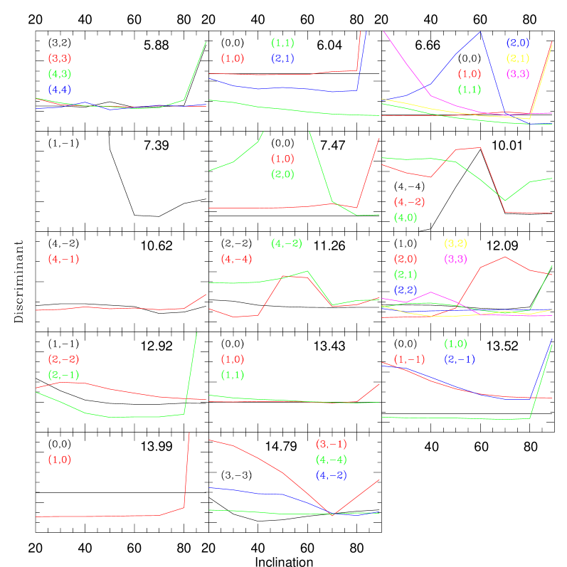
Figure 7: The discriminant of the best fitting modes are shown for each detected frequency term as a function of the inclination of the rotational axis. $\ell,m$ numbers are in the same colour of the corresponding line.

In order to evaluate the inclination, a total discriminant has been computed by adding for each inclination the minimum global discriminants of all the detected modes. As a matter of fact, the 7.39 cd^-1 mode dominates this discriminant and all the other modes supply only perturbations. Their presence affects appreciably this discriminant only for $i$ close to $90^{o}$. The result is reported in Fig. 8, where we see that there is a rather broad minimum centred at about $70^{o}$.

Figure 8: Total discriminant obtained summing the best discriminants of all the modes at each inclination versus the inclination angle.

Assuming this inclination, the equatorial rotational velocity results of about 73 km s^-1, and therefore the rotational period is about 2.4 d and the ratio between rotational and pulsation frequencies is lower than about 0.06 for all the modes.

Having established a reasonable value for the inclination angle, we can look at the discriminants of the individual modes in order to decide which are the more plausible identifications for this inclination. The proposed $\ell,m$ identifications for each detected mode are reported in the $6^{th}$ column of Table 7. For some modes these identifications are rather uncertain or there are different solutions which fit almost equivalently well the line profile variations. The more uncertain results are given between brackets.

In Fig. 9 we show the variations of the Ti 4501 line profile due to the 7.39 cd^-1 term (solid line) phased on a complete pulsation cycle and the corresponding best fitting variations generated by a model of a $\ell=1,m=-1$ mode. This model explains the 93% of the line profile variance, fits the $B$ light variations with a standard deviation of 0.4 mmag and the radial velocity variations with an accuracy of $\pm$0.2 km s^-1.

Figure 9: The variations induced on the profile of the TiII 4501 line by the 7.39 cd^-1 term phased over 1 cycle (solid lines) and the best fitting model of a mode with $\ell=1,m=-1$ and $i=70^{o}$ (dashed lines). The small bar at the lower left indicates a 0.02 amplitude in continuum intensity units.

In Fig. 10 we show the observed amplitude (upper panel) and phase variations (bottom panel) of the 7.39 cd^-1 term across the TiII line profile with the error bars derived from the least–squares fit, together with the corresponding curves derived from the best fitting model (solid lines). If we take into account all the approximations present in our model of pulsating star, we have to be more than satisfied by the quality of these results. Furthermore the figure makes it clear that the bump in the amplitude curve at the left of the line profile, that was already present in the 1992 data (see Fig. 4 of paper II), is a signature of the pulsation mode.

Figure 10: Observed (bars) and computed (solid lines) behaviours across the TiII 4501 line profile of the amplitude (top panel) and phase (bottom panel) of the 7.39 cd^-1 mode. The computed model correspond to the best fitting $\ell=1,m=-1$ mode, $i=70^{o}$.

5.5 Color phase shifts

In order to add weight to the mode identification a further independent tessera can be included in the mosaic by considering the phase differences between $V$ and $B$ light variations. Figure 11 shows this quantity versus the respective observed frequency for the 6 strongest photometric modes (namely, in order of frequency, 6.04, 6.66, 7.49, 7.47, 13.52 and 13.58 cd^-1). From the line profile variation analysis we have derived that apart from the 7.47 cd^-1 mode, all the others have as preferred choice $\ell=1$ (see Table 5). We see from the diagram that all of them fall in a strip of $\pm 3^{o}$ about the zero shift (dotted lines), just as expected. On the contary the 7.47 cd^-1 mode, for which the best option is $\ell=0$, has the highest fase difference and falls just outside this strip, again as expected.

Figure 11: Phase shifts between $V$ and $B$ light variations for the 6 strongest photometric modes. The dashed lines define the strip in which falls all the modes with $\ell=1$.

6 Discussion

6.1 Physical quantities related to pulsation modes

In the Table 5 we present the physical quantities obtained by fitting line profile and light variations for the better identified modes. In the successive columns we give: observed frequency ($\nu$), $\ell,m$, frequency in the stellar reference frame ($\nu_{0}$), pulsation constant ($Q$), amplitude of local radial velocity ($v_{r}$), percentual local flux variation ($\Delta F/F$) at the line wavelength, phase shift between flux and radial variation ($\psi$), percentual local radius variation ($\Delta R/R$), and the ratio between relative flux and radius variation ($f$). The reported amplitudes are sinusoidal amplitudes, so that the full amplitudes are twice these values.

Table 5: Physical parameters of the better identified modes

$\nu$	$\ell,m$	$\nu_{0}$	$Q$	$v_{r}$	$\Delta F/F$	$\Psi$	$\Delta R/R$	$f$
[cd-1 ]		[cd-1 ]	[d]	[km s-1]	%	[deg]	%
5.88	3,2	6.71	0.033	2.2	3.9	96	0.20	20
6.04	1,1	6.46	0.035	2.9	4.0	121	0.25	16
6.66	1,1	7.09	0.032	2.0	1.8	119	0.17	11
7.39	1,-1	6.98	0.032	25.1	19.0	114	2.04	9
7.47	0,0	7.47	0.029	2.4	2.0	102	0.18	11
11.26	2,-2	10.44	0.021	1.7	1.4	132	0.09	16
12.92	2,-1	12.51	0.018	6.3	5.1	145	0.29	18
13.52	1,0	13.52	0.016	5.1	3.6	149	0.22	16
13.99	1,0	13.99	0.016	9.5	7.2	164	0.39	18

The mode with the best defined parameters is obviously 7.39 cd^-1. We believe that these parameters are rather reliable: the formal uncertainties that we got from the simultaneous fit of its line profile and light variations are $\pm 1$ km s^-1  on $v_{r}$, $\pm 1.7\%$ on $\Delta F/F$, $\pm 7^{o}$ on $\Psi$, $\pm 0.09\%$ on $\Delta R/R$ and $\pm 1.0$ on $f$. It is interesting to compare the $f=9$ and $\Psi=114^{o}$ values with those predicted by theoretical models for a star with physical parameters similar to X Caeli. For low–degree $\ell$ modes of low radial order we have, for a mixing length parameter $\alpha=0.5$, $f\sim 11$ and $\Psi\sim 115^{o}$ and, for $\alpha=1.0$, $f\sim 8$ and $\Psi\sim 150^{o}$ (theses data were kindly supplied us by W. Dziembowsky, and the $f$ values have beeen rescaled at the line wavelength). The agreement with the theory is rather good, and it seems that our data favour a mixing length parameter of about 0.5.

The parameters of the other modes are more uncertain, given the small amplitudes of the perturbations produced by these modes on the line profiles.

It is worth noticing that the two lowest frequency modes (5.89, 6.04 cd^-1 ) are retrograde, as probably is also the case for the 6.66 cd^-1 one . Up to now there was not a large evidence of the presence of retrograde modes in $\delta$ Scuti stars: Kennelly et al. (1998) suspected that two high–degree modes in $\tau$ Peg could be retrograde, and Mantegazza and Poretti (1999) showed the presence of a rather certain low–degree retrograde mode in BB Phe.

We observe too, that the 6.66 and 7.39 cd^-1 terms have, within the approximations, due to the uncertaintinies on $i$ and on the Ledoux factor $C$, the same frequency in the stellar reference frame. Hence, having $\ell=1$, and $m=1$ and $m=-1$ respectively, they could be the rotational splitting of the same mode.

6.2 Fundamental stellar parameters as derived from pulsation

The identification of the 7.47 cd^-1 mode allows us to estimate some physical parameters of the star. As we have seen, this mode has been clearly detected in the light and in the radial velocity curves, but its detection is more uncertain in the line profile variations. Moreover its phase curve shows a clear rotation of $180^{o}$ in the line center, and the amplitude of the line profile variations are larger in the wings. These facts suggest that we are in presence of a mode that shifts the line rather than affecting its shape. Since in addition the mode is preferably seen in the integrated quantities and the inclination of the rotational axis is rather high, this mode is probably a radial mode. The same suggestion is supplied by its colour phase shift, even if on this basis alone we cannot rule out the $\ell=1$ possibility (Fig. 11).

If this is the correct identification then its $Q$ value as derived from the assumed physical parameters ($0.029\pm 0.004$ d) would put it midway between fundamental ($Q=0.033\pm 0.001$ d) and first overtone mode ($Q=0.025\pm 0.001$ d). In the first hypothesis the 7.39 cd^-1 term should be a $\ell=1$ $f$ mode, while according to the second it should be a $\ell=1$ $p_{1}$ mode (see the theoretical models by Fitch, 1981). In Table 6 we report the stellar fundamental parameters and their uncertainties as derived from three different hypotheses: a) adopting the Hipparcos parallax, b) 7.47 cd^-1 is the radial fundamental mode, c) 7.47 cd^-1 is the $1^{st}$ overtone radial mode. All the hypotheses assume the effective temperature derived from multicolor photometry, and the validity of the theoretical models by Shaller et al. (1992). In this table $\nu_{F}$ is the fundamental radial mode frequency. The uncertainty on the 7.47 cd^-1 mode ($\pm$0.02 cd^-1) is larger than on the other detected modes (see section 4) because of its proximity to the 7.39 cd^-1 mode.

Table 6: Physical parameters of the star estimated by considering the 7.47 cd^-1 mode as the radial fundamental or the first overtone mode and compared with the parameters derived using the Hipparcos parallax

	Hipparcos	Fund.	1st ov.
$T_{eff}$	$6900\pm 100$	$6900\pm 100$	$6900\pm 100$
$M/M_{\odot}$	$2.0\pm 0.1$	$1.90\pm 0.1$	$1.95\pm 0.05$
$M_{bol}$	$1.30\pm 0.15$	$1.47\pm 0.08$	$1.06\pm 0.08$
$R/R_{\odot}$	$3.45\pm 0.32$	$3.16\pm 0.08$	$3.82\pm 0.10$
$\log g$	$3.66\pm 0.09$	$3.72\pm 0.04$	$3.57\pm 0.04$
$\rho/\rho_{\odot}$	$0.049\pm 0.014$	$0.061\pm 0.004$	$0.036\pm 0.002$
$\nu_{F}$[cd-1 ]	$6.7\pm 0.7$	$7.47\pm 0.02$	$5.75\pm 0.02$
d[pc]	$102\pm 7$	$93\pm 3$	$113\pm 4$

The bolometric magnitude obtained with the fundamental mode assumption is $1\sigma$ higher than derived from Hipparcos parallax, while that obtained with the first overtone assumption is $1.4\sigma$ lower. On these bases it is difficult to get a firm conclusion even if it is slightly favoured the fundamental mode option for the 7.47 cd^-1 term. This without considering the possible presence of a circumstellar envelope that, introducing some extinction, could shift the result toward the first overtone mode hypothesis. In any case it can be appreciated how the use of the astroseismological information leads to a shrinking of the error bars.

Table 7: Complete list of the frequency terms detected in X Cae

freq.	Amplitude				$\ell,m$	Alt.Freq.	Possible
	V	B-V	RV	LP			couplings
[cd-1 ]	[mmag]		[km s-1]	[$10^{-3}$]	[cd-1 ]
5.89	1.8	0.3	0.2	1.6	3,2
6.04	7.6	1.9	0.7	2.7	1,1
6.22	1.4	0.0	0.1	—	—	7.16
6.66	3.9	1.2	0.4	1.7	1,1; 2,1	(7.67)
7.39	37.2	13.6	3.9	14.9	1,-1
7.47	5.6	1.9	0.5	1.5	0,0
8.85	1.4	0.2	—	—	—
10.01	0.6	1.4	0.2	2.4	(4,-4;4,-2)	9.01
10.62	1.2	0.7	—	1.5	(4,-2;4,-1)
11.26	0.9	0.3	0.1	1.8	2,-2	12.26?
11.77	1.9	1.0	0.2	—	—
12.09	1.8	0.1	0.2	1.7	2,1; 1,0		($\approx 6.04*2$)
12.92	3.3	0.6	—	2.1	2,-1
13.44	2.8	0.5	0.4	1.4	—		6.04+7.39
13.52	4.0	1.1	0.5	1.7	1,0; 0,0		($\approx 6.04+7.47$)
13.99	7.1	2.1	0.9	3.0	1,0
14.78	2.0	0.9	—	1.6	—		7.39*2

7 Conclusions

The analysis of the simultaneous photometric and spectroscopic observations of X Caeli has supplied the following results:

• 17 terms have been detected in the photometric data, most of which were already detected in the 1989 and 1992 campaigns. The comparison of the amplitudes of the strongest terms has shown that while the dominant mode (7.39 cd^-1 ) looks rather stable other terms have large amplitude variations.

• The analysis of the radial velocity curve detected 13 terms, and again 13 (but not exactly the same) were detected from the analyis of the line profile variations. All these terms are among those detected from photometry. Therefore no high–degree modes have been detected, even if the line profiles are sufficiently broadened by rotation to allow it.

• By means of simultaneous least–squares fits of the line profile and light variations induced by each mode we were able to supply $\ell,m$ identifications for many modes, and to estimate the inclination of the rotational axis (about $70^{o}$).

• The two shortest period modes are retrograde ones, while the 6.66 and 7.39 cd^-1 modes are probably the result of the rotational splitting of a $\ell=1$ mode.

• The physical parameters of the modes with the most reliable identifications have been given (Table 5). Rather accurate values have been obtained for the dominant mode, which has $\ell=1$, $m=-1$. When compared with those predicted by theoretical models they allow the estimation of the mixing length parameter which results about 0.5.

• The 7.47 cd^-1 mode is probably radial. It remains uncertain if it is the fundamental or the first overtone. The stellar physical parameters derived in both hypotheses are given and compared and discussed with those obtained using the Hipparcos parallax.

Table 7 summarizes all the detected modes in the present campaign with the different techniques and in order of increasing frequency. In the successive columns the $V$, $B-V$, RV amplitudes and the rms one across the line profile are given. The last three columns give furthermore the most probable $\ell,m$ identification, the eventual alternative frequency due to aliasing, and the possible relationships with the observed frequencies of other modes.

The research presented in this paper has supplied a lot of useful and interesting results concerning the pulsational behaviour and the physical characteristics of the $\delta$ Scuti star X Caeli. However a number of questions remains open and needs further investigations. First of all some of the detected terms still suffer of the 1 cd^-1 uncertainty which could probably be removed through a multisite photometric campaign.

Furthermore a better resolution both in spectroscopy and photometry would be useful to have a better plot of some close terms as the 7.39 and 7.47 cd^-1 . This would allow us to get a more accurate evaluation of the contribution of each mode to the observed variations and consequently would allow us to perform a more reliable mode identification. For instance the confirmation of the radial nature of the 7.47 cd^-1 mode would be of particular relevance in order to nail the fundamental stellar physical parameters.

Longer baselines would moreover allow us to detect more pulsation modes whose presence can be guessed from the present data, and to improve the accuracy of the phase shifts in different photometric bands and hence to allow an independent check of the $\ell$ identifications supplied by spectroscopy.

Given the brigthness of the object the use of a larger telescope in photometry would not significantly improve the results. However, since some modes produce variations of only a few thousands of the continuum intensity (see Fig. 6), a larger telescope in spectroscopy would allow us to obtain more accurate estimates of the line profile variations through higher $S/N$ data.

Nonetheless we emphasize that in order to improve the mode detection an effort should be made on the theoretical side too. Indeed, as Fig. 10 clearly shows, the computed amplitudes across the line profile of the best fitting mode ($1,-1$) for the dominant term (7.39 cd^-1), for which the spectroscopic $S/N$ is amply adequate, have still considerable systematic deviations from the observed amplitude variations.

- (1) Aerts C., 1996 A&A 314, 115
- (2) Balona L.A., 1986, MNRAS 220, 647
- (3) Balona L.A., 1987, MNRAS 224, 41
- (4) Bossi M., Mantegazza L., Nuñez N.S., 1998, A&A 336, 518
- (5) Breger M., Handler G., Nather R.E., et al., 1995, A&A 297,483
- (6) Breger M., Zima W., Handler G., et al. 1998, A&A
- (7) De Mey K., Daems K., Sterken C., 1998, A&A 336, 327
- (8) Dworetsky M.M., Moon T.T.,1986, MNRAS 220, 787
- (9) Fitch W.S., 1981, ApJ 249, 218
- (10) Hauck B., Mermilliod M., 1990, A&AS 40, 1
- (11) Heynderickx D., Waelkens C., Smeyers P., 1994, A&AS 105, 447
- (12) Kennelly E.J., Brown T.M., Kotak R. et al., 1998, ApJ 495, 440
- (13) Kunzli M., North P., Kurucz R.L., Nicolet B., 1997, A&AS 122, 51
- (14) Mantegazza L., Poretti E., 1992, A&A 255, 153
- (15) Mantegazza L., Poretti E., 1996, A&A 312, 855
- (16) Mantegazza L., 1997, A&A 323, 845
- (17) Mantegazza L., Poretti E., 1998, Proc. IAU Symp. 181, Poster Vol. p.267, Université de Nice
- (18) Mantegazza L., Poretti E., 1999, A&A 348, 139
- (19) Moon T.T., Dworetsky M.M., 1985, MNRAS 217, 305
- (20) Poretti E., Zerbi F.M., A&A 268, 369
- (21) Rufener F., 1988, Catalogue of stars measured in the Geneva Observatory Photometric System, Obs. Geneve
- (22) Schaller G., Schaerer D., Meynet G., Maeder A., 1992, A&AS 96, 269
- (23) Sperl M., 1998, Comm. in Asteroseismology (Vienna) 111, 1
- (24) Vaniĉek P., 1971, APSS 12, 10