An inverse Compton scattering (ICS) model of pulsar emission:
III. polarization

Abstract

Qiao and his collaborators recently proposed an inverse Compton Scattering (ICS) model to explain radio emission of pulsars. In this paper, we investigate the polarization properties of pulsar emission in the model. First of all, using the lower frequency approximation, we derived the analytical amplitude of inverse Compton scattered wave of a single electron in strong magnetic field. We found that the out-going radio emission of a single relativistic electron scattering off the “low frequency waves” produced by gap-sparking should be linearly polarized and have no circular polarization at all. However, considering the coherency of the emission from a bunch of electrons, we found that the out-going radiation from the inner part of emission beam, i.e., that from the lower emission altitudes, prefers to have circular polarization. Computer simulations show that the polarization properties, such as the sense reversal of circular polarization near the pulse center, S-shape of position angle swing of the linear polarization, strong linear polarization in conal components, can be reproduced in the ICS model.

Subject Headings: polarization — Pulsars: general — Radiation mechanisms: non-thermal

1 Introduction

The outstanding polarization properties of radio pulsars are keys to understand the magnetospheric structures of the neutron stars and the unknown emission mechanisms. Not only linear but also circular polarization has been detected from most pulsars. Soon after the discovery of pulsars, Radhakrishnan & Cook (1969) proposed the rotation vector model to interpret the rotating position angle of linear polarization, which has been widely accepted for practical reasons, regardless of the emission mechanism. Obviously, the linear polarization is probably related to the structure of the strong dipole field above magnetic poles. Large amount of polarization data have been accumulated (e.g. Gould & Lyne 1998; Manchester, Han & Qiao 1998; Rankin, Stinebring & Weisberg 1989; Weisberg et al. 1999). However, many observed polarization features can not be well explained, for example, the orthogonal position angles of linear polarization observed from individual pulses (e.g. Stinebring et al. 1984a,b), diverse circular polarization (e.g. Han et al. 1998), the different polarization characteristics of core and conal emission (Rankin 1993; Lyne & Manchester 1988). Though there were many theoretical efforts (e.g. Gil & Snakowski 1990), no consensus has ever reached on how pulsar polarization was generated (Radhakrishnan 1992; Melrose 1995). For example, the observed circular polarization in pulsar radio emission could either be converted from the linear polarization in the pulsar magnetosphere via the propagation effect (Melrose 1979, Cheng & Ruderman 1979; von Hoensbroech & Lesch 1999) or plasma process (e.g. Kazbegi et al. 1991), or origin from emission process intrinsically (Radhakrishnan & Rankin 1990; Michel 1987; Gangadhara 1997).

Recently, Qiao and his collaborators proposed an inverse Compton scattering (ICS) model of pulsar emission (Qiao 1988; Qiao & Lin 1998; Qiao et al. 1999). In the model, radio emission is the result of the secondary particles scattering off “low-frequency waves”. The waves are assumed to be produced by either the breaking down of the vacuum polar gap, or other sorts of short time oscillations or micro-instabilities (Björnsson 1996) . The gap-sparking may exist above polar cap, as shown by new observations by Deshpande & Rankin (1999) and by Vivekanand & Joshi (1999). If so, there must be low-frequency waves emitted by such sparking. The time scale of a sparking at a certain point is about $10^{-5}$ s or even shorter, the out-flowing plasma produced by the cascades of the sparking should form miniflux tubes with a radius of $\sim 10$ m and a length of $\sim 100$ m, and hence be highly inhomogenous in space. The plasma density between the tubes should be sufficiently low for radio wave to propagate, as if in a vacuum. Therefore, we assume that the pulsar magnetosphere is transparent for radio emission. That is to say, electromagnetic waves of observed emission can pass through the magnetosphere freely, and the so-called “low-frequency wave” can propagate through the emission region above the polar gap (see Qiao & Lin 1998). The success of the ICS model (Qiao & Lin 1998, Qiao et al. 1999) is that the core and the conal emission beams can be naturally explained in this model, while the core component comes from the nearest region to neutron-star surface, the inner cone is farther, and the out cone is farthest. Because of different heights of these emission components, the retardation and aberration effects cause the components apparently shift spatially, and could produce the position angle jumps in the integrated pulse profiles in some cases (e.g. Xu et al. 1997).

In this paper, we investigate the polarization properties of the ICS model for radio pulsars. First of all, we presented the polarization characteristics of scattered radio emission from a single particle in Sect. 2, half from theoretical work, half from numerical calculations. In the low frequency limit, deduction of the amplitude of outgoing radio waves from the ICS process in classical electrodynamics (CED) was presented in Appendix. In Sect. 3, we showed that the circular polarization can be the result of coherency of the outgoing waves. Considering the geometry above the polar cap regions, we numerically simulated the ICS process, and found that the circular polarization with possible sense reversal is preferably found from the emission in the beam center, while stronger linear polarization preferably from the outer part of the beam. Some related issues will be discussed in Sect. 4.

2 Polarization features of the out-going scattered waves from a single electron

The polarization features of scattered emission by relativistic electrons in the strong magnetic field has not been discussed in literature. In this section we are concerned with the general polarization properties of the scattered photons by a single relativistic electron onto the lower frequency waves. Previously, the quantum electrodynamics (QED) results of Compton scattering cross sections were first derived by Herold (1979) for electrons with ground initial and final states. Then, the QED cross sections for various initial and final electron states were calculated by Melrose & Parle (1983) and Daugherty & Harding (1986). Finally, Bussard, Alexander & Mesaros (1986) presented the QED results for electrons with arbitrary initial and final states. Xia et al. (1985) calculated for the first time the differential cross section of inverse Compton scattering, but no polarization features were discussed.

Based on the results of cross sections of various polarization vectors derived by Herold (1979), we used the Lorentz transformation in the magnetic field direction to calculate the differential cross section of inverse Compton scattering of orthogonal polarization pairs, an approach similar to that in Xia et al. (1985). Hereafter we denote the angular frequency of an incident photon as $\omega_{\rm in}$, the strength of magnetic field as $B$, and its cyclotron frequency as $\omega_{\rm c}={eB\over mc}$, and the angular frequency of the scattered wave or photon as $\omega_{\rm out}$. The geometry of the ICS process is shown in Fig. 1. The relativistic electron is moving along the field line (on the $z$ axis) and has a Lorentz factor $\gamma$ (and $\beta^{2}=1-1/\gamma^{2}$ in the equations) which we suppose to be about $\sim 10^{2}$ to $\sim 10^{3}$ in the pulsar magnetosphere. From the kinematic restrictions for the scattering process in strong magnetic fields, i.e. the momentum conservation in the magnetic field direction and the energy conservation of the process, the frequency of the scattered photons is (note that “$\sin\theta$” in Eq.(15c) of Xia et al. 1985 should read as“$\sin^{2}\theta$”)

$$\omega_{\rm out}=\left\{\begin{array}[]{ll}\omega_{\rm in}{\gamma(1+\beta)\over 2}{2\gamma mc^{2}(1-\beta\cos\theta_{\rm in})+\hbar\omega_{\rm in}\sin^{2}\theta_{\rm in}\over mc^{2}+\gamma\hbar\omega_{\rm in}(1+\beta)(1-\cos\theta_{\rm in})},&\theta_{\rm out}=0\\ \omega_{\rm in}{2\gamma mc^{2}(1-\beta\cos\theta_{\rm in})+\hbar\omega_{\rm in}\sin^{2}\theta_{\rm in}\over 2[\gamma(1+\beta)mc^{2}+\hbar\omega_{\rm in}(1+\cos\theta_{\rm in})]},&\theta_{\rm out}=\pi\\ {f(1-\sqrt{1-g})\over\hbar\sin^{2}\theta_{\rm out}},&\theta_{\rm out}\neq 0,\pi\end{array}\right.$$

where $f=\gamma(1-\beta\cos\theta_{\rm out})mc^{2}+(1-\cos\theta_{\rm in}\cos\theta_{\rm out})\hbar\omega_{\rm in}$ and $g=\hbar\omega_{\rm in}\sin^{2}\theta_{\rm out}[2\gamma(1-\beta\cos\theta_{\rm in})mc^{2}+\sin^{2}\theta_{\rm in}\hbar\omega_{\rm in}]/f^{2}.$ When $\hbar\omega_{\rm in}\ll m_{\rm e}c^{2}$, all above three equations can be simplified as being

$$\omega_{\rm out}=\omega_{\rm in}{1-\beta\cos\theta_{\rm in}\over 1-\beta\cos\theta_{\rm out}}.$$

According to the definition given by Saikia (1988), we derived the Stokes parameters (similar to Eq.(6) below) of scattered wave with the geometry plotted in Fig. 1. We numerically calculated the polarization properties, using Herold’s results, for radio frequency regime and high energy bands. We found that the polarization properties of the scattered photons are different.

(1). When $\omega_{\rm in}\ll\omega_{c}$ and both $\omega_{\rm in}$ and $\omega_{\rm out}$ are in radio band, the scattered photons are completely linearly polarized, and its polarization position angle (PA) is definitely in the co-plane of the out-going photon direction and the magnetic field (see geometry in Fig. 1), in spite of the polarization state of incident photons with one exception for the very specific case in which the incident photon is absolutely linear polarized and its polarization vector is exactly perpendicular to the magnetic field line.

We derived the amplitude of the scattered waves from a single electron with the classical electrodynamics (CED), which we will use in next sections for emission coherence. The electron can be considered as a particle since the magnetic field $B\ll B_{q}$, here $B_{q}$ is the critical magnetic field $B_{q}=(m^{2}c^{3})/(e\hbar)=4.413\times 10^{13}$ G, and the incident and the scattered photons can be considered as waves since the frequency of the incident wave in the electron-rest-frame is much smaller than the resonant frequency, i.e., $\omega_{\rm in}\gamma(1-\beta\cos\theta_{\rm in})\ll\omega_{c}$. We derived (see Appendix) that the electric field ${\bf E}_{\rm s}(t)$ of the scattered wave is

$${\bf E}_{\rm s}(t)=-{r_{\rm c}\over D}E_{0}\frac{\cos\eta\sin\theta_{\rm in}\sin\theta_{\rm out}}{\gamma^{2}(1-\beta\cos\theta_{\rm out})^{2}}e^{i({\bf k}\cdot{\bf D}-\omega_{\rm out}t)}\cdot{\bf e}^{\rm out}_{1},$$

where ${\bf k}$ the wave-vector, ${\bf D}$ the position vector from scattering electron to observer, $r_{\rm c}$ the electron classical radius. The incident wave has electric field amplitude $E_{0}$, and its electric vector has an angle $\eta$ with respect to ${\bf e}^{\rm in}_{1}$. The wave is scattered to be the out-going wave with only completely linear polarization, the polarization vector of which (${\bf e}^{\rm out}_{1}$) is in the plane of out-gong wave and magnetic field, in consistent with the results from the QED calculation shown above. We note that Chou & Chen (1990) have calculated Stokes parameters of Thomson scattered wave in strong magnetic fields and found that the scattered radiation is always linearly polarized for any polarized incident wave. Their results serve as an independent check of the specific case of $\gamma=1$ above.

In 3-D, emission from a single electron is going out in a micro-cone around the magnetic line, the cross-section profile is shown in Fig. 2, with the maximum at about $\theta_{\rm out}={1\over\sqrt{3}\gamma}\simeq$0.6/$\gamma$ (i.e. $0.3^{\circ}$ when $\gamma=100$. See Fig. 2), as deduced from Eq. (A9). At this angular radius, the frequency of the scattered waves should be (from Eq. 2)

$$\omega_{\rm out}=1.5\;\omega_{\rm in}\gamma^{2}(1-\beta\cos\theta_{\rm in}).$$

When a line-of-sight goes across the micro-cone, one can detect an “S” shape variation of polarization angle. Note that this cross section of the micro-cone does not have a gaussian-shape. All those polarization properties do not vary with frequency until $\omega_{\rm in}$ is about $10^{14}$ s^-1.

(2). For resonant scattering at high energy bands (for $B=10^{12}$G, $\omega_{\rm in}=1.3\;10^{18}$ s^-1), the scattered emission ($\omega_{\rm out}=1.7\;10^{21}$ s^-1) has a filled gaussian-like shape with the total emission peak in the direction of magnetic field (see Fig. 3), rather than a micro-cone. Circular polarization is 100% near the center, but decreases to zero when the angular radius $\theta_{\rm out}$ is about $1/\gamma$, and it changes the sense and gets almost 100% again when $\theta_{\rm out}=1.5/\gamma$. In contrast, there is no linear polarization near the center and the edge, but it peaks up to almost 100% when $\theta_{\rm out}=1/\gamma$. The position angle of linear polarization of the scattered photon is perpendicular to the co-plane of out-going photon and the magnetic field, different from the case in radio band.

(3). When $\omega_{\rm in}$ is about the resonant frequencies, i.e. higher than about $10^{14}$ s^-1 or lower than $10^{20}$ s^-1 as seen in Fig. 4, the total intensity of the scattered photons increases towards the resonant frequency. However, this increased total intensity is mainly contributed from circularly polarized emission, which is shown in the upper plots of Fig. 4 from the fraction variations of circular polarization with frequency at given directions of out-going photons.

What we considered in the second and third cases is at high energy regime with parameters $B=10^{12}$G and $\gamma=100$ in this section. However, polarization properties of scattered emission we presented above should be the same for the situation in the resonant region in the outer magnetosphere of pulsars which we will not considered in this paper.

Note that all these conclusions for an electron are the same for a positron because the amplitude of the scattered waves rests on the incident waves, having nothing to do with the charge sign of a particle.

3 The coherent ICS process in pulsar magnetosphere

Strong polarization is the most outstanding feature of pulsar emission. Circular polarization has been detected from pulsars, and sometimes has sense-reversals across pulse profile (Han et al. 1998). In this section, we consider the pulse polarization in the frame of the ICS model.

As we see from the last section, scattered emission in radio band from a single electron is completely linearly polarized, and the position angle follows an “S” shape for a sweep of the line of sight. The scattered waves from electrons in a close group are coherent, which can produce the circular polarization detected from pulsars. The amplitude of coherent emission can be calculated by using Eq. (3) for radio emission, so that we can avoid the much more complicated procedures by using coherent states in quantum electrodynamics. For example, if two linearly polarized plane waves E₁ and E₂ with same wave vector have a phase difference $\delta$ and an angle of $\kappa$ between their polarization vectors, the circular polarization percentage of the coherently superimposed emission is

$${V\over I}={2E_{1}E_{2}\sin\kappa\sin\delta\over E_{1}^{2}+E_{2}^{2}+2E_{1}E_{2}\cos\kappa\cos\delta}.$$

For $E_{1}=E_{2}$, Eq.(4a) becomes

$$V/I=\sin\kappa\sin\delta/(1+\cos\kappa\cos\delta).$$

This gives considerably circular polarization, as long as the values of $|\sin\kappa|$ and $|\sin\delta|$ are not too small. If $\kappa=\delta=\pi/2$, it will be totally circularly polarized.

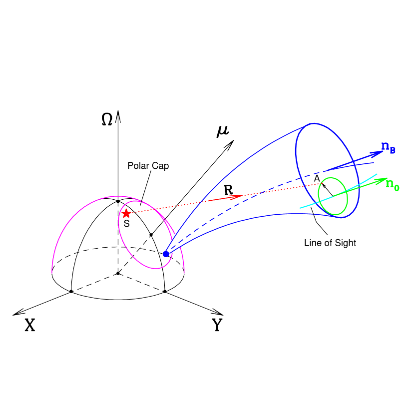
Figure 5: The geometry of the coherent ICS process. The sparking occurs at a point S above the polar cap, and produces the incident waves that are scattered by a bunch of particles. The emission visible to an observer at n₀ is from a ring-like area satisfying ${\bf n}_{B}\cdot{\bf n}_{0}\sim\cos(0.6/\gamma)$. Point $A$ is on this ring.

In the ICS model of radio emission of pulsars, the incident waves were generated by a sparking due to the breaking down of inner gap. The waves travel through a vacuum-like pulsar magnetosphere with a small filling factor of pair plasma (i.e., inhomogenous spatially). They encounter a bunch of relativistic particles that come from another cascade (in the other side) above the polar cap, and are upscattered coherently (Fig. 5) to produce the observed radio emission. In a given observational direction, coherently superpose scattered waves from a bunch of particles, which is seen from the transient “mini-beam” below, can be almost completely linearly polarized or some times have very strong circular polarization dependent on geometry. This is mainly the result of the coherency and the non-random distributions of the $\delta$ and $\kappa$ in Eq.(4). However, the observed integrated pulse profiles of pulsars, is the incoherent sum of many samplings of these mini-beams. In the field of view of a given line of sight, if the sparkings distribute symetrically, the circular polarizations will cancel each other, and no circular polarization left finally. Nevertheless, there is remarkable circular polarization in mean pulses if the sparking distribution is asymmetric.

In this section, we first describe the coherent ICS process of a bunch of particles, then we present computer simulations of their transient beam. Finally we simulate the mean pulse profiles, which have linear and circular polarization, S-shaped position angle swing and unpolarized emission as well.

3.1 The scattered waves from a bunch of particles

The scattered emission from a single particles is in a micro-cone of about $0.6/\gamma$ (see Fig. 2 and Sect. 2), hence only emission from a small area is visible to a given line-of-sight ${\bf n}_{0}$. Since a particle is moving in a direction along the magnetic field ${\bf n}_{\rm B}$, the emission from these particles satisfying ${\bf n}_{B}\cdot{\bf n}_{0}\sim\cos(0.6/\gamma)$ can be received by an observer. Using Eq.(2a) (see also Eq.(6) of Qiao & Lin 1998), combined with Eqs.(11) and (13) of Qiao & Lin (1998) which describe the scattering geometry and how the Lorentz factor of the particles changes along the field lines, one can find three emission heights for a given frequency. At a certain observing frequency, an observer cannot receive emission at the same time from all zones at three heights produced by a bunch of particles, but just see a part of one zone .

The upper-scattered waves from particles in such a small area can be accumulated coherently for some good reasons. First of all, the low frequency incident waves that were generated by one sparking should have a phase coherence when they encounter the bunch of particles, even if with a small phase dispersion due to travelling. Secondly, the scattered waves at one given frequency from these particles in a small visible ring-like area would have a good phase coherence as well. The complex electric field amplitude contributed from each particle[see Eq.(3)] reads

$${\bf E_{s}}=C{\cos\eta\sin\theta_{\rm in}\over R}\exp[{\it i}({\omega_{\rm in}\over{\it c}}R-{\omega_{\rm out}\over{\it c}}{\bf R}\cdot{\bf n_{0}}+\phi_{0})]\;{\bf e}_{1}^{\rm out},$$

here $C$ is a constant for a given $\gamma$. Vectors R = SA and n₀ are illustrated in Fig.5, and $\phi_{0}$ is the initial phase of the incident waves when it was generated by a sparking. Note that $\phi_{0}$ might be random for different sparkings. When the incident waves come from one sparking, we can integrate the complex amplitudes (rather than the power) from Eq. (3a) of scattered waves from all visible particles. The complex electric field amplitude of the total scattered wave is,

$${\bf E}=\int_{{\bf n}_{B}\cdot{\bf n}_{0}\sim\cos(0.6/\gamma)}{\bf E}_{\rm s}\;n_{\rm e}\;dV.$$

Here, $n_{\rm e}$ is the number density of particles in the bunch. The Stokes parameters of this accumulated emission are (Saikia 1988)

$$\left\{\begin{array}[]{lll}I&=&{1\over 2}[({\bf e}_{10}\cdot{\bf E})^{*}({\bf e}_{10}\cdot{\bf E})+({\bf e}_{20}\cdot{\bf E})^{*}({\bf e}_{20}\cdot{\bf E})],\\ Q&=&{1\over 2}[({\bf e}_{10}\cdot{\bf E})^{*}({\bf e}_{10}\cdot{\bf E})-({\bf e}_{20}\cdot{\bf E})^{*}({\bf e}_{20}\cdot{\bf E})],\\ U&=&{\rm Re}[({\bf e}_{10}\cdot{\bf E})^{*}({\bf e}_{20}\cdot{\bf E})],\\ V&=&{\rm Im}[({\bf e}_{10}\cdot{\bf E})^{*}({\bf e}_{20}\cdot{\bf E})].\end{array}\right.$$

Two orthogonal polarization vectors above were defined to be ${\bf e}_{20}={\bf n}_{0}\times{\bf\Omega}/|{\bf n}_{0}\times{\bf\Omega}|,$ and ${\bf e}_{10}={\bf e}_{20}\times{\bf n}_{0}$, here $\Omega$ is the direction of rotation axis (Fig. 5).

3.2 Transient beam from a bunch of particles: simulation

We now simulate the coherent ICS process of a bunch of particles, and will present its 2-D emission feature snap-shot.

The particles produced by the sparkings are moving out along the extremely strong magnetic fields. The radius of a sparking spot was assumed to have the same scale as the inner gap height (Gil 1998) , which Deshpande & Rankin (1999) estimated to be about 10 meters. We took this value in the following simulations, but we have found that changing of this dimensional size does not affect our results. We also assumed that the number density of particles $n_{\rm e}$ in a bunch has the maximum in the center and decline towards the edge. We took a gaussian distribution for convenience. This number density will be the natural weight upon the contribution in Eq.(5) from different visible part of a ring-like area at a given frequency. The wave-phase of this contribution depends on the location of this visible part relative to a sparking spot.

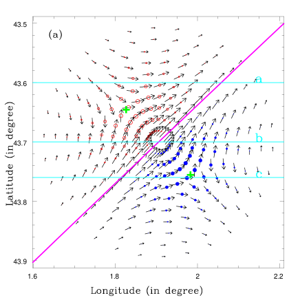
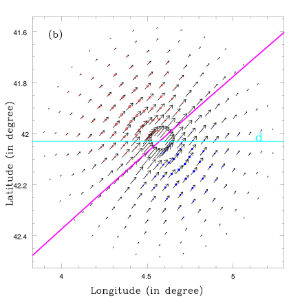
Figure 6: Polarization features of transient (a) core and (b) inner conal minibeams. The vectors stand for the polarization vector, their length is proportional to intensity. The filled and open circles represent the circular polarization of two senses, their size is proportional to circular polarization percentage. The circular polarization at two points in the core minibeam marked by the crosses gets to the maximum of 100%, with position angle jumps and null linear polarization. The sizes of circle in Fig.6b have been amplified by 4 times for clarity. The thick line is the projection of the curved magnetic field. The line of sight goes across the beam, for example, along lines $a$, $b$ and $c$ in Fig. 6a and $d$ in Fig. 6b. The radius of bunch is $R_{\rm b}=10$ m, magnetic inclination angle $\alpha=45^{\circ}$, the bunch location $\phi_{\rm c}=225^{\circ}$, and $\gamma_{0}=2000$, $\omega_{\rm out}=1$ GHz.

The ICS process by one bunch of particles moving along given field lines forms three “mini-beams” of a few degrees in width. They were produced at emission heights of core and two cones, respectively. We assumed that the particles in the bunch have the same Lorentz factor, and found that the polarization features are quite different between these mini-beams(see Fig. 6).

As seen in Fig. 6, circular polarization is very strong, even up to 100%, in the core minibeam, as shown by the open and filled circles. Emission from the minibeam of inner cone is much less circularly polarized. However, we could not calculate the beam feature of the outer cone using coherent superposition method as in the case of core and inner cone, since the particles at this larger emission height have much smaller Lorentz factors, and therefore the visible ring-like area (see Fig. 5) is so large that the upscattered emission is no longer coherent.

We also made simulations for a bunch of particles with different Lorentz factors, but the polarization features shown in Fig.6 do not change significantly. This does not surprise us since the global polarization pattern is mainly determined by field geometry.

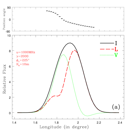
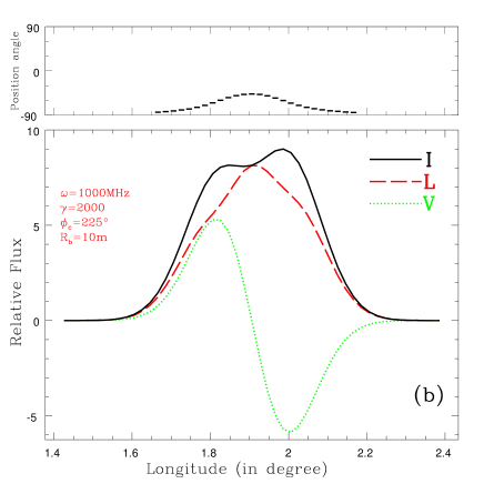
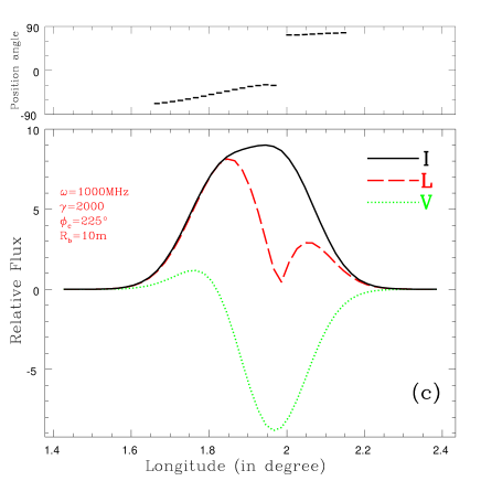
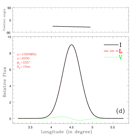
Figure 7: Cross-sections of transient beams, cut by the lines of sight $a$, $b$, $c$ and $d$ in Fig 6. The obvious features of these “subpulses” are the presence of different circular polarization patterns and the variation of position angles. The circular polarization percentage and position angle variation range of inner cone emission (d) both are much less than that of core emission (a, b, c).

When the line of sight sweeps across a minibeam, we can see a transient “subpulse”, as shown in Fig. 7. Note that the width of “transient” subpulses is about $0.6^{\circ}$, much larger than $1/\gamma\sim 0.04^{\circ}$. When the line of sight sweeps across the center of a core or inner conal minibeam, the circular polarization will experience a central sense reversal, or else it will be dominated by one sense, either left hand or right hand according to its traversal relative to the minibeam.

The position angles at a given longitude of transient “subpulses” have diverse values around the projection of the magnetic field (see Fig.6 and Fig.7). The variation range of position angles is larger for core emission, but smaller for conal beam. When many such “subpulses” from one minibeam is summed up, the mean position angle at the given longitude will be averaged to be the central value, which is determined by the projection of magnetic field lines. Therefore in our model, the mean position angle of pulsar emission beam naturally reflects the geometry of magnetic field lines. As we will show in our simulation the position angle of mean pulse profiles should have “S” shapes (see section 3.3).

Note that these transient “subpulses” are not the subpulse we observe from pulsars. The time scale for the transient beam to exist is very short, about $10^{-5}$ s. A real observation sample with extremely high time resolution (e.g. a few $\mu$s) will detect one point from only one transient “subpulse”. In this case, a strong (even near 100%) circular polarization could be observed. Observational evidence was presented by Cognard et al. (1996). However, if sampling time is longer (e.g. ms), what one receive is the incoherent summation of emission from hundreds of transient beams at a given longitude. This largely diminishes the circular polarization, but does not affect much on the linear one.

3.3 Polarization features of integrated pulse profiles

Integrated profiles of pulsars are characterized by linear polarization, circular polarization, the sweep of position angle, and substantial amount of unpolarized emission. Our simulation shows these characters can all be reproduced. In our model, at every longitude, an observer can see the scattered emission from particles in the many sparking-produced bunches around his line of sight. To get the integrated profile, we sum up incoherently the Stokes parameters of the scattered waves from all these bunches. For the simplicity of simulation, we assumed the particles in one bunch have the same Lorentz factor, since changing the Lorentz factor or considering the energy distribution of these particles should not alter the results following.

We used the geometry presented in Fig. 5 for our model calculation, which helped to determine the different $\theta_{\rm in}$ values for a sparking to every bunch in the ICS process. The key factor is the distribution of sparking spots in the polar cap. In the inner gap, a sparking is triggered when a $\gamma$-photon encounters considerable $B_{\bot}$, namely the perpendicular component of magnetic field, and produces an $e^{\pm}$ pair. A pair production cascade forms and the inner gap is discharged. This seems more likely to occur in a peripheral parts of the polar cap due to large $B_{\bot}$ while the central parts are inconducive to discharge. But at the edge of the gap, there is null electric field and thus it is impossible for a sparking to occur (Ruderman & Suthland 1975). Therefore, the preferred region of gap discharge is located between the center and the edge on the polar cap. We assume in our simulation that the sparking spots have a gaussian distribution radially from the magnetic axis, with a maximum at $\theta\sim 0.75\theta_{\rm pc}$, where $\theta_{\rm pc}$ is the radius of the polar cap. However, changing the form of this radial distribution will not affect our results qualitatively.

In the inner gap model, the electric potential across the gap is produced via monopolar generation. When the magnetic axis inclines from the rotation axis, the potential which accelerates the particles are different in the part of gap nearer to the rotation axis compared to that in the further part. Therefore, the probability of polar gap discharging varies with the distance to the rotation axis. This distribution asymmetry with respect to the magnetic axis has been included in our simulations. The probability of the sparkings was assummed to decrease exponentially with the azimuthal angle from the projection of the rotational axis. It is several times larger in the nearest part to the rotation axis than that in the farthest part.

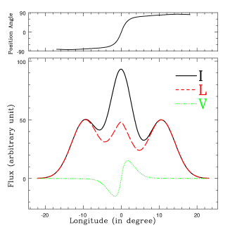
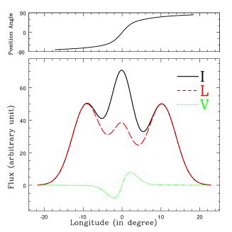
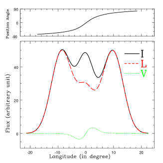
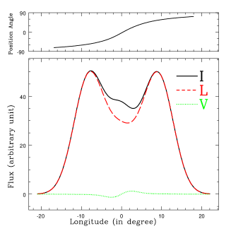
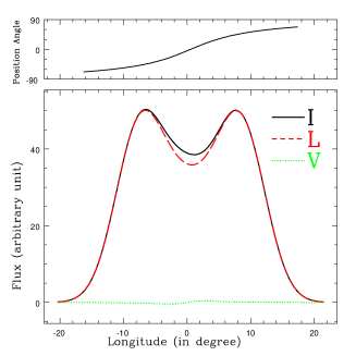
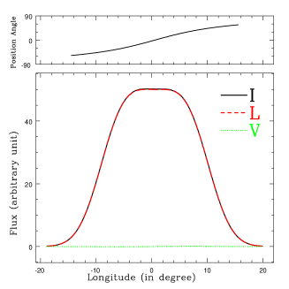
Figure 8: A set of integrated pulse profiles, simulated for the normalized impact angle $\beta_{\rm n}=0.15$, 0.30, 0.45, 0.60, 0.75, and 0.9. An S-shaped position angle swing, linear polarization, an antisymmetric type of net circular polarization and substantial amount of unpolarized emission can be presented from the ICS model. A small beam-shift between core and conal components due to different emission heights has been included in the simulation.

In Fig.8, we present a set of polarization profiles with various impact angle $\beta$. We found that the integrated profiles are highly linear polarized in general, and their polarization angles follow nice S-shapes. One can immediately see that the position angle curves have a larger “maximum sweep rate” for a smaller $\beta$, in excellent accordance with the rotating vector model.

One important result is the antisymmetric circular polarization found in the central or core component, which can be up to 20%. As we mentioned before, circular polarization can be up to 100% on some part of “subpulses”, but depolarization occurs in the process of incoherent summation of circular polarization of opposite senses. This also produces a substantial amount of unpolarized emission. For the linearly polarized emission, position angles of transient “subpulses” vary, causing further depolarization.

However, in the conal components, circular polarization is insignificant, mainly because it is originally weak in the minibeam (see Sect.3.2). Since there is negligible variation of position angles of “subpulse”, almost no linear depolarization presents, and therefore, the conal components are always highly linearly polarized.

4 Discussion and Conclusions

Qiao (1988) and Qiao & Lin (1998) proposed an inverse Compton scattering model for radio pulsar emission. The simulations presented in this paper show that linear as well as circular polarization can be obtained from coherent inverse Compton scattering process from a bunch of particles, although the radio radiation of a single electron is highly linearly polarized. In the simulation process, there are two assumptions we have made, namely the coherence of the outgoing waves and small velocity dispersion of particles in a bunch. The circular polarization is favorable to be produced in emission regions near the polar cap in the ICS model. Observational data show that the ‘core’ emission is radiated at a place relatively close to the surface of the neutron star (Rankin 1993), the ‘inner cone’ is emitted in a higher region, and the ‘outer cone’ in the highest. Our simulations show that circular polarization tends to appear in the core components, while the ‘outer cone’ emission is linearly polarized.

One might have noticed that the circular polarization from our simulation of the ICS model is always strong and antisymmetric in the central part of integrated pulsar profiles. It is of intrinsic origin. However, almost no circular polarization appears in the conal components according to the ICS model, therefore the observed one must be converted from the strong linear polarization in propagation process (Radhakrishnan & Rankin 1990; Han et al. 1998; von Hoensbroech & Lesch 1999).

One important ingredient to produce the circular polarization in the ICS model is the non-radial asymmetry of sparking distribution. We found from our summation that, without the non-radial asymmetry, circular polarization will be canceled by incoherent summation. The same conclusion has been reached by Radhakrishnan & Rankin (1990) when they studied circular polarization using curvature radiation.

The polarization of the individual pulses or micro-pulses, however, should be related to the time resolution of observations according to the ICS model. With high time resolution (e.g. short to $\sim 10\mu$s), each sample will take emission from few transient beam that has strong linear and circular polarization. Depolarization happens during the sample time of a low resolution. This can serve as a test for our model.

We emphasize that the width of observed subpulses is not necessary associated with $1/\gamma$ suggested by Radhakrishnan & Rankin (1990). The width of real subpulses observed from pulsars is generally 2-3 degrees, which was used to estimate $\gamma$ to be less than several tens. In our simulation, the width of transient “subpulse” produced by a bunch of particles along certain field lines reflect the width of the minibeam, which is mainly determined by the dimension of the bunch. The bunch radius near the star surface was taken to be 10 meters, corresponding to about one degree in longitude for core emission, and a little bit larger for cones. The width of a real observed sub-pulse might be related to the dimension of magnetic tube for the bunches more often to flow-out. Therefore, the upper limit of $\gamma$ can be released to $10^{3}$ or even higher.

In our simulation, the low-frequency waves are assumed to be monochromatic. We have also made simulations for various $\omega_{\rm in}$, and found that the polarization properties of transient beam and integrated profiles are quite similar to the results we presented above.

Appendix: The amplitude of scattered wave in strong magnetic field

We consider the complex amplitude of scattered wave in the electron-rest-frame, and then make Lorentz transformation for our case. The equation of motion for an electron with $\gamma=1$ in a magnetic field $B$ is

$$m\stackrel{{\scriptstyle..}}{{\bf r}}=e{\bf E}(t)+{e\over c}\stackrel{{\scriptstyle.}}{{\bf r}}\times{\bf B}.$$

Here, $e$ is the electron charge, and $c$ is the speed of light. For conditions $|\dot{\bf r}|\ll c$ and $\omega_{\rm in}\ll\omega_{c}$, the magnetic component of the incident wave and the radiation damping force have been neglected. The electric field of the incident wave is taken as ${\bf E}(t)={\bf E}_{0}\exp({-i\omega_{\rm in}t})={\bf e}^{\rm in}\;E_{0}\exp({-i\omega_{\rm in}t})$ (here ${\bf e}^{\rm in}$ is the polarization vector for incident wave) and the position vector of the electron as ${\bf r}(t)={\bf r}_{0}\exp({-i\omega_{\rm in}t})$. Generally, ${\bf E}_{0}$ and ${\bf r}_{0}$ are complex vectors. One then can get

$$m\omega_{\rm in}^{2}{\bf r}_{0}+e{\bf E}_{0}-i{e\omega_{\rm in}\over c}{\bf r}_{0}\times{\bf B}=0.$$

For the incident wave in $x$-$z$ plane (see Fig.1), fundamental linear polarization vectors of incident wave were defined ${\bf e}^{\rm in}_{1}=\{-\cos\theta_{\rm in},\;0,\;\sin\theta_{\rm in}\}$ and ${\bf e}^{\rm in}_{2}=\{0,\;-1,\;0\}$. The magnetic field ${\bf B}=\{0,\;0,\;B\}$. The fundamental vectors of scattered waves were chosen to be ${\bf e}^{\rm out}_{1}=\{-\cos\theta_{\rm out}\cos\phi,\;-\cos\theta_{\rm out}\sin\phi,\;\sin\theta_{\rm out}\}$, and ${\bf e}^{\rm out}_{2}=\{\sin\phi,\;-\cos\phi,\;0\}$. See Fig. 1 for the parameters of geometry. For a given incident wave, ${\bf e}^{\rm in}=\cos\eta{\bf e}^{\rm in}_{1}+\sin\eta{\bf e}^{\rm in}_{2}$. Here ${\bf e}^{\rm in}$ is a complex vector, and hence $\eta$ is a complex number generally. One can get the solutin of Eq.(A1) as:

$${\bf r}_{0}={\nu r_{c}\over 1-\mu^{2}}\left(\begin{array}[]{l}\cos\eta\cos\theta_{\rm in}+i\mu\sin\eta\\ \sin\eta-i\mu\cos\eta\cos\theta_{\rm in}\\ \cos\eta\sin\theta_{\rm in}(\mu^{2}-1)\end{array}\right),$$

here $\mu\equiv\omega_{c}/\omega_{\rm in}$, $\nu\equiv E_{0}c^{2}/(e\omega_{\rm in}^{2})$, and $r_{c}={e^{2}\over mc^{2}}$. In case of strong magnetic field, $\mu\gg 1$, and if $\eta\neq\pi/2$, Eq.(A.3) can be simplified as being

$${\bf r}_{0}=\{0,\;0,\;-\nu r_{c}\cos\eta\sin\theta\}.$$

The electric field for the scattered wave can be written as (for $|\dot{\bf r}|\ll c$)

$$\begin{array}[]{lll}{\bf E}_{\rm s}(t)&=&{e\over cD}[{\bf n}\times({\bf n}\times\stackrel{{\scriptstyle..}}{{\bf r}})]_{\rm ret}\\ &=&-{r_{\rm c}\over D}E_{0}\cos\eta\sin\theta_{\rm in}\sin\theta_{\rm out}\;\exp[i{\omega_{\rm in}\over c}({\bf n}\cdot{\bf D}-ct)]\;{\bf e}^{\rm out}_{1}.\end{array}$$

Here, ${\bf n}=\{\sin\theta_{\rm out}\cos\phi,\;\sin\theta_{\rm out}\sin\phi,\;\cos\theta_{\rm out}\}$ and ${\bf D}$ is the position vector from a scattering point to an observer, $D={|{\bf D}|}$. From Eq.(A.5) one see that the scattered wave has only the term of ${\bf e}^{\rm out}_{1}$, and there is no ${\bf e}^{\rm out}_{2}$ term, which implies the completely linear polarization of the scattered waves. The differential cross section is

$$d\sigma_{\eta}={E_{s}^{2}D^{2}d\Omega_{\rm out}\over E_{0}^{2}}=r_{c}^{2}\cos^{2}\eta\sin^{2}\theta_{\rm in}\sin^{2}\theta_{\rm out}d\Omega,$$

here $d\Omega_{\rm out}$ is the solid angle of the scattered wave. The total cross section is

$$\sigma_{\eta}=\int d\sigma_{\eta}=\sigma_{\small\rm Th}\cos^{2}\eta\sin^{2}\theta_{\rm in},$$

here, $\sigma_{\small\rm Th}={8\pi\over 3}r_{c}^{2}$ is the Thomson section. For $\eta=0$ (i.e. just for one polarization of ${\bf e}^{\rm in}_{1}$), one can get $\sigma|_{\eta=0}=\sigma_{\small\rm Th}\sin^{2}\theta_{\rm in}$, which is consistent with the Eq.(16) at the lower frequency limit ($\omega_{\rm c}\gg\omega_{\rm in}$) in Herold’s (1979) when ${\omega\over\omega_{\rm B}\pm\omega}=0$.

In the extreme case of $\eta=\pi/2$, the value of $|{\bf r}_{0}|$ is extremely small (with a factor of $(\omega_{\rm in}/\omega_{\rm c})^{2}$) for the scattered waves in the radio band, so we will not discuss it in following.

For an electron with $\gamma>1$, one can easily found through Lorentz transformation that the polarization vector of a wave is the same in an alternative inertial frame, but the complex amplitude of electric field of the wave in moving frame is $\gamma(1-\beta\cos\theta_{\rm in})$ times that in a rest frame. In the electron rest frame (the frame moving with a electron with Lorentz factor $\gamma$), the complex amplitude of the electric field for the incident wave is $E_{0}^{\small R}=\gamma(1-\beta\cos\theta_{\rm in})E_{0}$. The complex amplitude for the scattered wave in the electron rest frame is $E_{\rm s}^{\small R}=-{r_{\rm c}\over D}E_{0}\cos\eta\sin\theta_{\rm in}\sin\theta_{\rm out}/[\gamma(1-\beta\cos\theta_{\rm out})]$, hence, in the laboratory frame it becomes

$$E_{\rm s}=\gamma(1+\beta\cos\theta_{\rm out}^{\small R})E_{s}^{\small R}\\ =-{r_{\rm c}\over D}E_{0}\cos\eta\sin\theta_{\rm in}\sin\theta_{\rm out}[\gamma(1-\beta\cos\theta_{\rm out})]^{-2}.$$

Therefore, for a moving electron with Lorentz factor $\gamma$, the electric field of the scattered wave becomes

$${\bf E}_{s}(t)=-{r_{\rm c}\over D}E_{0}\cos\eta\sin\theta_{\rm in}\sin\theta_{\rm out}\;[\gamma(1-\beta\cos\theta_{\rm out})]^{-2}\;\exp[i{\omega_{\rm in}\over c}({\bf n}\cdot{\bf D}-ct)]\;{\bf e}^{\rm out}_{1}.$$

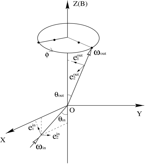
Figure 1: The geometry of the ICS process for a single electron. The incident photon is coming as $\omega_{\rm in}$ in the x-z plane, and the scattered photons are going out around the magnetic field line (i.e., the $z$ axis). The geometrical parameters used in the rest of the paper have been marked. In x-z plane, $\phi=0$.

Figure 2: The total and linearly polarized intensities vary with the distance from the field direction, forming an micro-cone of out-going photons. The curves were calculated for $\theta_{\rm in}=30^{o}$ and $80^{o}$. Other parameters were taken as: $B=0.1B_{q}$ (here $\omega_{c}=7.75\;10^{19}$ s^-1), $\gamma=100$, $\omega_{\rm in}=10^{5}$ s^-1.

Figure 3: The resonantly scattered waves: the total, linear and circular polarization intensity varying with the distance from the magnetic field direction were plotted as a solid line, dashed line and dash-dot-dash line, respectively.

Figure 4: The frequency dependence of total intensity (lower plots) and circular polarization percentage (upper plots) of the scattered waves about the resonant frequency, in four given directions of the out-going photon beam as $(\phi,\theta_{\rm out})=(0^{\circ},0.5/\gamma)$, $(45^{\circ},0.5/\gamma)$, $(0^{\circ},2.0/\gamma)$, and $(45^{\circ},2.0/\gamma)$. See Fig. 1 for geometry. The solid lines are plotted for the azimuthal angle $\phi=0^{\circ}$, and dash-dot-dot-dot lines for $\phi=45^{\circ}$. The left is plotted for emission at the angular radii $\theta_{\rm out}=0.5/\gamma$, and the right for $\theta_{\rm out}=2/\gamma$.

References

- (1)
- (2) Björnsson, C.-I., 1996, ApJ, 471, 321
- (3)
- (4) Bussard, R. W., Alexander, S. B., Mesaros, P. 1986, Phys. Rev., D34, 440
- (5)
- (6) Cheng, A.F., Ruderman, M.A., 1979, ApJ 229, 348
- (7)
- (8) Chou, C. K., & Chen, H. H. 1990, ApSS, 174, 217
- (9)
- (10) Cognard I., Shrauner J.A., Taylor J.H., Thorsett S.E., 1996, ApJ 457, L81
- (11)
- (12) Daugherty, J. H., & Harding, A. K. 1986, ApJ, 309, 362
- (13)
- (14) Deshpande, A.A, & Rankin, J.M. 1999 ApJL, in press
- (15)
- (16) Gangadhara R.T., 1997, A&A 327, 155
- (17)
- (18) Gil, J.A., Snakowski, J.K., 1990, A&A, 234, 237
- (19)
- (20) Gil, J. A., 1998, in: 1997 Pacific Rim Conference on Stellar Astrophysics, eds: K. L. Chan, K. S. Cheng, & H. P. Singh, Astronomical Society of the Pacific Conference Series, Vol. 138, p. 109
- (21)
- (22) Gould, D. M., Lyne, A.G., 1998, MNRAS 301, 235
- (23)
- (24) Han, J. L., Manchester, R. N., Xu, R. X., & Qiao, G. J., 1998, MNRAS, 300, 373
- (25)
- (26) Herold, H. 1979, Phys. Rev. D19, 1868
- (27)
- (28) Kazbegi, A.Z., Machabeli, G.Z. & Melikidze, G.I. 1991, MNRAS, 253, 377
- (29)
- (30) Lyne, A.G., & Manchester, R.N., 1988, MNRAS 234, 477
- (31)
- (32) Manchester, R.N., Han, J.L., Qiao, G.J., 1998, MNRAS 295, 280
- (33)
- (34) Melrose, D. B., 1979, Aust. J. Phys., 32, 61
- (35)
- (36) Melrose, D. B., 1995, J. Astrophy. Astron. 16, 137
- (37)
- (38) Melrose, D. B., & Parle, A. J. 1983, Aust. J. Phys., 36, 755
- (39)
- (40) Michel F.C., 1987, ApJ 322, 822
- (41)
- (42) Qiao, G. J., 1988, Vistas in Astronomy, 31, 393
- (43)
- (44) Qiao, G. J., Lin, W. P., 1998, A&A 33, 172 (Paper I)
- (45)
- (46) Qiao, G.J., Liu, J.F., Zhang, B., and Han, J.L., 1999, ApJ submitted (Paper II)
- (47)
- (48) Radhakrishnan, V., 1992, in: The Magnetosphere Structure and Emission Mechanism of Radio Pulars, Hankin T. et al. (eds), Proc. of IAU Colloq. No.128, p.367
- (49)
- (50) Radhakrishnan V., & Cooke D. J., 1969, Ap.L. 3, 225
- (51)
- (52) Radhakrishnan, V., & Rankin, J. M., 1990, ApJ., 352, 258
- (53)
- (54) Rankin, J. M., 1993, ApJ 405, 285
- (55)
- (56) Rankin, J. M., Stinebring, D.R., Weisberg, J.M., 1989, ApJ 346, 869
- (57)
- (58) Ruderman, M. A. & Sutherland, P. G. 1975, ApJ 196, 51
- (59)
- (60) Saikia, D. J., 1988, Ann. Rev. A&Ap., 26, 93
- (61)
- (62) Stinebring, D. R., Cordes, J. M., Rankim, J. M., Weisberg, J. M., & Boriakoff, V., 1984a, ApJS, 55, 247
- (63)
- (64) Stinebring, D. R., Cordes, J. M., Weisberg, J. M., Rankin, J. M., & Boriakoff, V., 1984b, ApJS, 55, 279
- (65)
- (66) Vivekanand, M., & Joshi, B. C. 1999 ApJ 515, 398
- (67)
- (68) von Hoensbroech, A., Lesch, H., 1999, A&A 342, L57
- (69)
- (70) Weisberg J.M., Cordes J.M., Lundgren S.C., et al., 1999, ApJS 121, 171
- (71)
- (72) Xia, X. Y., Qiao, G. J., Wu, X. J., & Hou, Y. Q. 1985, A&A, 152, 93
- (73)
- (74) Xu, R. X., Qiao, G. J. & Han J. L. , 1997, A&A, 323, 395
- (75)