Distribution of Caustic-Crossing Intervals for
Galactic Binary-Lens Microlensing Events

Abstract

Detection of caustic crossings of binary-lens gravitational microlensing events is important because by detecting them one can obtain useful information both about the lens and source star. In this paper, we compute the distribution of the intervals between two successive caustic crossings, $f(t_{\rm cc})$, for Galactic bulge binary-lens events to investigate the observational strategy for the optimal detection and resolution of caustic crossings. From this computation, we find that the distribution is highly skewed toward short $t_{\rm cc}$ and peaks at $t_{\rm cc}\sim 1.5$ days. For the maximal detection of caustic crossings, therefore, prompt initiation of followup observations for intensive monitoring of events will be important. We estimate that under the strategy of the current followup observations with a second caustic-crossing preparation time of $\sim 2$ days, the fraction of events with resolvable caustic crossing is $\sim 80\%$. We find that if the followup observations can be initiated within 1 day after the first caustic crossing by adopting more aggressive observational strategies, the detection rate can be improved into $\sim 90\%$.

1 Introduction

Several groups are searching for massive astronomical compact objects (MACHOs) by monitoring light variations of stars caused by gravitational microlensing towards the Galactic bulge and the Magellanic Cloud fields (EROS: Aubourg et al. 1993; MACHO: Alcock et al. 1993; OGLE: Udalski et al. 1993; DUO: Alard & Guibert 1997). With their efforts, more than 400 candidate events have been detected to date.

Among these events, a considerable number of events are believed to be caused by binary lenses (Udalski et al. 1994a; Dominik & Hirshfeld 1994, 1996; Mao & Di Stefano 1995; Alard, Mao, & Guibert 1995; Bennett et al. 1996; Rhie & Bennett 1996; Alcock et al. 1999b; Afonso et al. 2000). The light curve of a binary-lens event differs from that of a single-lens event. The most distinctive feature of a binary-lens event light curve occurs when a source star crosses a lens caustic. When the source star is located on the caustic, the amplification becomes very large. Therefore, the light curve of a caustic-crossing binary-lens event is characterized by a sharp spike. On the other hand, if a binary-lens event does not involve a caustic crossing, the resulting light curve exhibits a relatively small deviation from that of a single-lens event (Mao & Paczyński 1991; Dominik 1998).

Detection of caustic-crossing binary-lens events is important because they can provide useful information both about the lens and source star. First, a caustic-crossing event provides an opportunity to measure how long it takes for the caustic line to transit the face of the source star. By using the source crossing time along with an independent determination of the source star size, one can determine the lens proper motion with respect to the source star (Afonso et al. 1998; Albrow et al. 1999a; Alcock et al. 1999a). With the determined lens proper motion, one can significantly better constrain the physical parameters of the lens (Gould 1994; Nemiroff & Wickramasinghe 1994; Witt & Mao 1994; Peng 1997). Second, a caustic-crossing event can also be used to determine the surface structure of the source star such as the radial brightness profiles (Gaudi & Gould 1999; Albrow et al. 1999b, 2000; Afonso et al. 2000) and spots (Han et al. 1999). To obtain these useful information from the light curve of a binary-lens event, the event should be monitored with high time resolution. However, under the nightly monitoring observational strategy of the current lensing experiments, it is difficult to construct light curves with resolution high enough to resolve caustics.

However, the caustic crossing can be resolved with the help of alert system based on real time observations (Alcock et al. 1996, 1997; Udalski et al. 1994b) and subsequent high time resolution followup observations (GMAN: Pratt et al. 1996; PLANET: Albrow et al. 1998; MPS: Rhie et al. 1998). Since the caustics of a binary-lens event form a closed curve, the source star of a caustic-crossing event crosses the caustic line at least twice. Although the first caustic crossing is unlikely to be resolved due to its short duration, it can be inferred from the enhanced amplification. Then, if followup observations can be prepared before the second caustic crossing, dense enough sampling through the second caustic will be possible. Therefore, it is important to estimate the distribution of the intervals between caustic crossings (caustic-crossing intervals, $t_{\rm cc}$) for the optimal detection and resolution of caustic crossings.

The distribution of caustic-crossing intervals, $f(t_{\rm cc})$, was computed by Honma (1999) for events expected towards the Magellanic Cloud field. His intention for the computation of $f(t_{\rm cc})$ was to demonstrate the detection bias against events with short $t_{\rm cc}$, for which the second caustic crossings are more likely to be missed. For this purpose, it was enough to determine $f(t_{\rm cc})$ based on the typical values of the lens mass and the Einstein ring radius crossing time (Einstein time scale, $t_{\rm E}$). However, for the investigation of the optimal observational strategy to detect and resolve caustic crossings, it is required to determine $f(t_{\rm cc})$ based on the distribution of Einstein time scales expected from detailed models of the physical and dynamical distributions of lens matter and binary mass function. In addition, since majority of caustic-crossing binary-lens events have been detected towards the Galactic bulge (Alcock 1999b), constructing $f(t_{\rm cc})$ for these events is desirable.

In this paper, we compute the distribution of the intervals between two successive caustic crossings, $f(t_{\rm cc})$, for Galactic bulge binary-lens events to investigate the observational strategy for the optimal detection and resolution of caustic crossings. From this computation, we find that the distribution is highly skewed toward short $t_{\rm cc}$ and peaks at $t_{\rm cc}\sim 1.5$ days. For the maximal detection of caustic crossings, therefore, prompt initiation of followup observations for intensive monitoring of events will be important. We estimate that under the strategy of the current followup observations with a second caustic-crossing preparation time of $\sim 2$ days, the fraction of events with resolvable caustic crossing is $\sim 80\%$. We find that if the followup observations can be initiated within 1 day after the first caustic crossing by adopting more aggressive observational strategies, the detection rate can be improved into $\sim 90\%$.

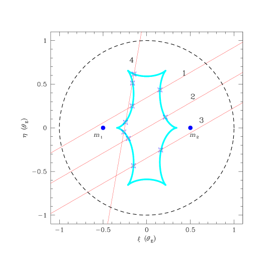
Figure 1: Caustic crossings for various source star trajectories (thin solid straight lines) for an example event caused by a binary system with a separation $\ell=1.0$ and a mass ratio $q=1.0$. The caustics are represented by a thick sold line. The location of the lenses ($m_{1}$ and $m_{2}$) are marked by dots and the circle drawn by a dashed line represents the combined Einstein ring.

2 Caustic-Crossing Intervals

2.1 Binary-lens Events

When the lengths are normalized to the combined Einstein ring radius, the lens equation in complex notations for a binary-lens system is represented by

$$\zeta=z+{m_{1}\over\bar{z}_{1}-\bar{z}}+{m_{2}\over\bar{z}_{2}-\bar{z}},$$

where $m_{1}$ and $m_{2}$ are the mass fractions of individual lenses (and thus $m_{1}+m_{2}=1$), $z_{1}$ and $z_{2}$ are the positions of the lenses, $\zeta=\xi+i\eta$ and $z=x+iy$ are the positions of the source and images, and $\bar{z}$ denotes the complex conjugate of $z$ (Witt 1990). The combined Einstein ring radius is related to the total mass $M$ of the binary system and its location between the observer and the source star by

$$r_{\rm E}=\left({4GM\over c^{2}}{D_{ol}D_{ls}\over D_{os}}\right)^{1/2},$$

where $D_{ol}$, $D_{ls}$, and $D_{os}$ are the separations between the observer, lens, and source star. Since the individual microlensing images cannot be resolved due to the small separations between them, the amplification of the binary-lens event is given by the sum of the amplifications of the individual images, $A_{i}$, which are given by the Jacobian of the transformation (1) evaluated at the image position, i.e.

$$A_{i}=\left({1\over|{\rm det}\ J|}\right)_{z=z_{i}};\qquad{\rm det}\ J=1-{\partial\zeta\over\partial\bar{z}}{\overline{\partial\zeta}\over\partial\bar{z}}.$$

The caustic refers to the source position on which the amplification becomes infinity, i.e. ${\rm det}\ J=0$. The set of caustics form a closed curve, called cautsics. The caustics take various shape and size depending on the binary mass ratio $q=m_{1}/m_{2}$ and the projected binary separation $\ell$ normalized by the angular Einstein ring radius $\theta_{\rm E}=r_{\rm E}/D_{ol}$. In Figure 1, we present the caustics (a thick solid curve) of an example binary-lens event with $\ell=1.0$ and $q=1.0$. In the figure, the locations of the lenses ($m_{1}$ and $m_{2}$) are marked by dots and the circle with its center at the center of mass of the binary system drawn by a dashed line represents the combined Einstein ring. For more example caustics of binary-lens events with various values of $\ell$ and $q$, see Figure 1 of Han (1999).

2.2 Distribution of Caustic-Crossing Separations

The caustic-crossing interval is proportional to the separation between two successive caustic-crossing points (caustic-crossing separation, $\theta_{\rm cc}$). Due to the dependency of the shape and size of the caustics on the binary separation and the mass ratio, the caustic-crossing separation and the resulting caustic-crossing interval depend on the values of $\ell$ and $q$. In addition, since $t_{\rm cc}$ is scaled by the Einstein time scale, which depends on the physical lens parameters of the mass, the location, and the lens-source transverse speed $v$ by

$$t_{\rm E}={r_{\rm E}\over v}=\left({4GM\over c^{2}v^{2}}{D_{ol}D_{ls}\over D_{os}}\right)^{1/2},$$

the caustic-crossing interval depends also on these parameters. Therefore, for the determination of $f(t_{\rm cc})$, one should consider binary-lens events which are expected for all combinations of $\ell$ and $q$ over the entire range of the physical lens parameters.

To determine $f(t_{\rm cc})$, we first determine the distribution of the caustic-crossing separations $f(\theta_{\rm cc};\ell,q)$, which is expected for events caused by a binary lens with $\ell$ and $q$. By defining a binary-lens event as a close lens-source encounter within the combined Einstein ring, we produce a large number of source trajectories that pass through the combined Einstein ring. The source star trajectory orientations with respect to the projected binary axis, $\psi$, and the impact parameter, $\beta$, are randomly selected in the ranges of $0\leq\psi\leq 2\pi$ and $0\leq\beta\leq 1$, respectively. If the source star trajectory crosses the lens caustics, we then find the crossing points and measure the separation $\theta_{\rm cc}$ in units of $\theta_{\rm E}$. In most cases, the source crosses the caustics twice, e.g. the three trajectories numbered by 1, 2, and 3 in Figure 1. But due to the concavity of the caustics, crossings can occur more than twice, e.g. the trajectory numbered by 4 in Figure 1. For these cases, we measure $\theta_{\rm cc}$ between every pair of two successive crossing points.

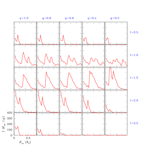
Figure 2: The distributions of the normalized caustic-crossing separations for events caused by binary systems with various separations $\ell$ (also normalized by $\theta_{\rm E}$) and mass ratios $q$. The individual distributions are arbitrarily normalized, but they are relatively scaled so that the area under each distribution is proportional to the caustic-crossing probability.

In Figure 2, we present the distributions $f(\theta_{\rm cc};\ell,q)$ for events caused by binaries with various projected separations and mass ratios. The individual distributions are arbitrarily normalized, but they are relatively scaled so that the area under each distribution is proportional to the caustic-crossing probability. From the figure, one finds that the distribution $f(\theta_{\rm cc};\ell,q)$ depends strongly, both in the scale (i.e. the caustic-crossing probability) and the shape, on the binary separation. In the scale, the caustic probability becomes maximum for binary-lens events with $\ell\sim 1.5$. This is because caustics at around this binary separation form the largest curve. With the same reason, the distribution peaks at relatively large caustic-crossing separations, e.g. at around $\theta_{\rm cc}=0.4$ for binary-lens events with $\ell\sim 1.5$. As the separation becomes smaller or larger, the caustics becomes smaller, making the caustic-crossing probability smaller and the distribution peaks at small value of $\theta_{\rm cc}$. On the other hand, the dependency of $f(\theta_{\rm cc};\ell,q)$ on the binary mass ratio both in the scale and the shape is relatively weak (Gaudi & Gould 1999).

With the obtained distribution of $f(\theta_{\rm cc};\ell,q)$, we then obtain the combined distribution of caustic-crossing separations by

$$f(\theta_{\rm cc})=\int_{0}^{1}dqf(q)\int_{0}^{\infty}dbf(\theta_{\rm cc};\ell,q)f(b)\delta(\theta_{\rm cc}-\theta_{\rm cc}^{\prime}),$$

where $f(q)$ and $f(b)$ respectively are the distributions of the binary mass ratios and the intrinsic binary separations $b$ in units of $\theta_{\rm E}$, and $\delta$ denote the delta function. The projected binary separation $\ell$ is obtained from the intrinsic separation $b$ by assuming that the intrinsic binary separation vector ${\bf b}$ is randomly oriented onto the sky. The notation $\theta_{\rm cc}^{\prime}$ represents the caustic-crossing separation obtained under the assumption of random orientation of ${\bf b}$. For the distribution $f(q)$, we adopt the distribution determined by Trimble (1990).

2.3 Distribution of Caustic-Crossing Intervals

Once the distribution of caustic-crossing separations $f(\theta_{\rm cc})$ is obtained, the distribution of the caustic-crossing intervals expected for events caused by binaries with a constant mass $M$ is obtained by

$$f(t^{\prime}_{\rm cc})=\int_{0}^{d_{\rm max}}dD_{os}\rho(D_{os})\int_{0}^{D_{os}}dD_{ol}\rho(D_{ol})\left({D_{ol}D_{ls}\over D_{os}}\right)^{1/2}$$

$$\times\int dv_{y}\int dv_{z}vf(v_{y},v_{z})\int_{0}^{\infty}d\theta_{\rm cc}f(\theta_{\rm cc})\delta\left(t^{\prime}_{\rm cc}-\theta_{\rm cc}t_{\rm E}\right),$$

where $\rho(D_{os})$ and $\rho(D_{ol})$ are the mass density of source stars and lenses along the line of sight toward the Galactic bulge, $d_{\rm max}$ is the maximum extent of the source star distribution, $(v_{y},v_{z})$ are the two components, parallel and normal to the Galactic plane, of the lens-source transverse velocity v, and $f(v_{y},v_{z})$ represents their distribution. In the equation, the factors $(D_{ol}D_{ls}/D_{os})^{1/2}$ and $v$ are included to weight $f(t^{\prime}_{\rm cc})$ by the cross section of the lens-source encounter, i.e. the Einstein ring radius $r_{\rm E}\propto(D_{ol}D_{ls}/D_{os})^{1/2}$, and the transverse speed.

For the matter distributions of the Galactic bulge, we adopt a ‘revised COBE’ model, which is based on a triaxial COBE model (Dwek et al. 1995) except the central part of the bulge. For the inner $\sim 600\ {\rm pc}$ of the bulges, we adopt a high central density Kent (1992) model which better matches with observations in this region. For the matter distributions of the Galactic disk, we adopt a double exponential disk model with vertical and radial scale heights of $h_{R}=325\ {\rm pc}$ and $h_{z}=3.5\ {\rm kpc}$ (Bahcall 1986). The transverse velocity distributions for both Galactic bulge and disk lenses are modelled by a Gaussian of the form

$$f(v_{i})\propto\exp\left[-{\left(v_{i}-\bar{v}_{i}\right)^{2}\over{2\sigma_{i}}^{2}}\right];\qquad i\in y,z,$$

where the means and the standard deviations for individual transverse velocity components are $({\bar{v}_{y}},\sigma_{y})$=(220,30) ${\rm km\ s}^{-1}$ and $({\bar{v}_{z}},\sigma_{z})$=(0,20) ${\rm km\ s}^{-1}$ for the disk lenses, and $({\bar{v}_{y}},\sigma_{y})$=(220,93) ${\rm km\ s}^{-1}$ and $({\bar{v}_{z}},\sigma_{z})$=(0,79) ${\rm km\ s}^{-1}$ for the bulge lenses, respectively. For the detailed discussion both about the matter and the transverse velocity distributions, see Han & Gould (1996).

The expected distributions of $f(t^{\prime}_{\rm cc})$ for events caused by various values of the binary mass are presented in the upper panel of Figure 3. In the lower panel, we also present the integrated probability for events with $t>t^{\prime}_{\rm cc}$, i.e. $P(t>t^{\prime}_{\rm cc})=1-\int_{0}^{t}f(t^{\prime}_{\rm cc})dt^{\prime}_{\rm cc}/\int_{0}^{\infty}f(t^{\prime}_{\rm cc})dt^{\prime}_{\rm cc}$. In each panel, to better show the distribution in the short caustic-crossing interval region, we expand the region and present in a separate small box. From the figure, one finds that as the binary-lens mass decreases, the distribution becomes narrower and peaks at shorter $t_{\rm cc}$.

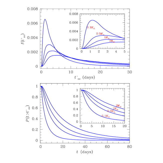
Figure 3: Upper panel: The distributions of caustic-crossing intervals for Galactic bulge events caused by binaries with various constant masses. Lower panel: The integrated probability for caustic-crossing events with $t>t^{\prime}_{\rm cc}$. In each panel, to better show the short $t^{\prime}_{\rm cc}$ region, we expand the region and presented in a separate small box.

Binary-lens events are caused by Galactic binaries with various masses. Then the final distribution of the caustic-crossing intervals is obtained by convolving $f(t^{\prime}_{\rm cc})$ with the mass function of binary lenses $\Phi_{\rm bi}(M)$, i.e.

$$f(t_{\rm cc})=\int dMM^{1/2}\Phi_{\rm bi}(M)\int_{0}^{\infty}dt^{\prime}_{\rm cc}f(t^{\prime}_{\rm cc})\delta(t_{\rm cc}-M^{1/2}t^{\prime}_{\rm cc}).$$

The factor $M^{1/2}$ in the first integrand is included to weight $f(t_{\rm cc})$ by the cross-section of lens-source encounter ($r_{\rm E}\propto M^{1/2}$), while the same factor in the second integrand is included because the caustic crossing-crossing interval is scaled by the Einstein time scale ($t_{\rm E}\propto M^{1/2}$).

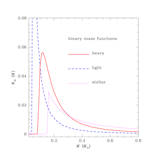
Figure 4: The model binary-lens mass functions that are used for the determination of the caustic-crossing interval distributions.

The mass function of binary lenses is very uncertain due to the observational difficulties in identifying binaries by resolving their components combined with our ignorance about the mechanism of binary formation. Furthermore, since binary-lens microlensing events can be caused by binaries which are composed of dark components (either one or both), construction of $\Phi_{\rm bi}(M)$ becomes even more complicated. Though many possibilities have been proposed, the scenarios for the formation of binaries can be classified into two categories. The first one is that binaries are formed during the star formation stage through fragmentation of a collapsing object (Norman & Wilson 1970; Boss 1988). In the other scenario, by contrast, both binary components form independently and then later combine through some sort of capture mechanism (Fabian, Pringle, & Rees 1975; Press & Teukolsky 1997; Ray, Kembhavi, & Anita 1987). Due to the difference in the binary formation mechanism, the mass functions expected from the two scanarios would be different each other. Under the formation environments of the former scenario, the most probable binary-lens mass function would be similar to that of single lenses. On ther other hand, under the circumstances of the latter binary formation scenario, the two lens masses would be drawn independently from the same mass function, which is similar to the single-lens mass function. For the construction of $f(t_{\rm cc})$, therefore, we test both binary mass function models expected under the two cases of binary formation scenario. The first binary mass function is modeled by a power law with a mass cutoff, i.e.

$$\Phi_{\rm bi}(M)\propto M^{-p}\Theta(m-m_{\rm cut}),$$

where $\Theta$ is a heavy side step function. For the values of the power and the mass cutoff, we adopt $p=2.1$ and $m_{\rm cut}=0.04\ M_{\odot}$, following the best-fitting values determined from the distribution of Einstein time scales of 51 Galactic bulge single-lens events by Han & Gould (1996). The second model of binary mass function is constructed by selecting masses of individual binary components from the same mass function in equation (9) and then combining the two masses. Since two masses are combined to yield a single binary mass, binaries following the latter mass function tend to be heavier than the binary lens masses following the former mass function. We distinguish the two models by calling them ‘heavy’ and ‘light’ binary mass functions. Note that since the mass cutoff of both the heavy and light binary mass functions is less than the hydrogen-burning limit of $0.08\ M_{\odot}$, dark component of lenses are included in these mass functions. In the third model, we test binary mass function which is constructed under the assumption that lenses are composed of only stars: ‘stellar’ mass function. We construct the stellar mass function by adopting the mass function determined by Zoccali et al. (2000) from observations of Galactic bulge stars by using the Hubble Space Telescope (HST) plus the Near Infrared Camera and Multi Object Spectrometer (NICOMOS). The stellar binary-lens mass function extends down to $0.15\ M_{\odot}$. In Figure 4, we present the model binary-lens mass functions.

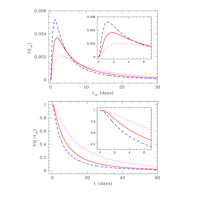
Figure 5: The resulting distributions of caustic-crossing intervals (lower left panel) and the integrated probabilities with $t>t_{\rm cc}$ for Galactic bulge binary-lens events determined for the two model binary-lens mass functions in the upper panel.

In Figure 5, we present the finally determined distribution of caustic-crossing intervals and integrated probability with $t>t_{\rm cc}$. From the figure, one finds that the distributions $f(t_{\rm cc})$ are highly skewed toward short $t_{\rm cc}$ regardless of the assumed mass functions. The peak of the distribution occurs at $\sim 1.5\ M_{\odot}$ although ther exist slight variations depending on the assumed binary-lens mass functions. As a result, majority (70%–90%) of binary-lens events expected to be detected towards the Galactic bulge will have caustic-crossing intervals shorter than $t_{\rm cc}=20$ days.

3 Discussion

In the current strategy, intensive followup observations of the second caustic crossing of a binary-lens event can be initiated within $\sim 2$ days after the first crossing. The primary search teams alert on the first caustic crossing within 1 day, and the followup teams begin monitoring of the event immediately. For example, the PLANET group generally produces template images the same day and is able to make rudimentary measurements of the event within a day after the receipt of the alert from the primary search teams. Once these rudimentary measurements of the event are in place, one can determine a second crossing time without difficulties. Therefore, the typical response time of the current followup observation teams is 2 days if the weather is good (A. Gould 1999, private communication). According to the determined distribution $f(t_{\rm cc})$, then, the fraction of binary-lens events whose second caustic crossings can be monitored by the followup observations is $\sim 80\%$ although there exist slight difference depending on the assumed mass functions. Therefore, we find that for Galactic bulge events the detection bias toward long time-scale events argued by Honma (1999) will not be very strong. However, we note that his argument about the detection bias against short time-scale events is based on the assumption that the current preparation time for intensive followup observations is greater than 7 days. We are not certain why his adopted preparation time is that long. However, if the same preparation time of 2 days is adopted, the fraction of LMC binary-lens events that can be intensively monitored by followup observations would be similar to that of Galactic bulge events.

However, the expected most frequent caustic-crossing interval of $\sim 1.5$ day is shorter than the current preparation time of the followup observations. Then, if the preparation time is shortened by adopting more aggressive observational strategy, one can detect and resolve caustic crossings for more binary-lens events. With the help of automatized process, the MACHO group (Alcock et al. 1997) can finish data reduction within 6 hrs of image acquisition. With vigorous efforts to minimize the preparation time, therefore, initiation of followup observations within 1 day after the first caustic crossing will be possible. We find that if the followup observations can be initiated within 1 day after the first caustic crossing, the detection rate can be improved into $\sim 90\%$.

References

- [1] Afonso, C., et al. 1998, A&A, 337, L17
- [2] Afonso, C., et al. 2000, ApJ, 532, 000
- [3] Alard, C., Mao, S., & Guibert, J. 1995, A&A, 300, L17
- [4] Alard, C., & Guibert, J. 1997, A&A, 326, 1
- [5] Albrow, M. D., et al. 1998, ApJ, 509, 687
- [6] Albrow, M. D., et al. 1999a, ApJ, 512, 672
- [7] Albrow, M. D., et al. 1999b, ApJ, 522, 1011
- [8] Albrow, M. D., et al. 2000, ApJ, submitted (astro-ph/9910307)
- [9] Alcock, C., et al. 1993, Nature, 365, 621
- [10] Alcock, C., et al. 1996, ApJ, 463, L67
- [11] Alcock, C., et al. 1997, ApJ, 491, 436
- [12] Alcock, C., et al. 1999a, ApJ, 518, 44
- [13] Alcock, C., et al. 1999b, ApJ, submitted
- [14] Aubourg, E., et al. 1993, Nature, 365, 623
- [15] Bahcall, J. N. 1986, ARA&A, 24, 577
- [16] Boss, A. P. 1988, Comments Astrophysics, 12. 169
- [17] Bennett, D. P., et al. 1996, Nucl. Phys. Proc. Suppl., 51B, 152
- [18] Dominik, M. 1998, A&A, 329, 361
- [19] Dominik, M., & Hirshfeld, A. C. 1994, A&A, 289, L31
- [20] Dominik, M., & Hirshfeld, A. C. 1996, A&A, 313, 841
- [21] Dwek, E., et al. 1995, ApJ, 445, 716
- [22] Fabian, A. C., Pringle, J. E., & Rees, M. J. 1975, MNRAS, 172, 15
- [23] Gaudi, B. S., & Gould, A. 1999, ApJ, 513, 619
- [24] Gould, A. 1994, ApJ, 421, L71
- [25] Han, C. 1999, MNRAS, 308, 1077
- [26] Han, C., & Gould, A. 1996, ApJ, 467, 540
- [27] Han, C., Kim, H.-I., Chang, K., & Park, S.-H. 1999, MNRAS, submitted
- [28] Honma, N. 1999, ApJ, 511, L29
- [29] Kent, S. M. 1992, ApJ, 387, 181
- [30] Mao, S., & Di Stefano, R. 1995, ApJ, 440, 22
- [31] Mao, S., & Paczyński, B. 1991, ApJ, 374, L37
- [32] Nemiroff, R. J., & Wickramasinghe, W. A. D. T. 1994, ApJ, 424, L21
- [33] Norman, M. L., & Wilson, J. R. 1978, ApJ, 224, 479
- [34] Peng, E. 1997, ApJ, 475, 43
- [35] Pratt, M. R., et al. 1996, in Proc. IAU Symp. 173: Astrophysical Applications of Gravitational Lensing, eds. C. S. Kochanek & J. N. Hewitt, (Dordrecht: Kluwer Academic Publisher), 221
- [36] Press, W. H., & Teukolsky, S. A. 1997, ApJ, 213, 183
- [37] Ray, A., Kembhavi, A. K., & Anita, H. M. 1987, A&A, 184, 164
- [38] Rhie, S. H., & Bennett, D. P. 1996, Nucl. Phys. Proc. Suppl., 51B, 86
- [39] Rhie, S. H., et al. 1998, BAAS, 193, 108.05
- [40] Schneider, P., & Weiss, A. 1986, A&A, 164, 237
- [41] Trimble, V. 1990, MNRAS, 242, 79
- [42] Udalski, A., et al. 1993, Acta Astro., 43, 289
- [43] Udalski, A., et al. 1994a, ApJ, 436, L103
- [44] Udalski, A., et al. 1994b, Acta Astro., 44, 227
- [45] Witt, H. J. 1990, A&A, 263, 311
- [46] Witt, H. J., & Mao, S. 1994, ApJ, 430, 505
- [47] Zoccali, M., Cassisi, S., Frogel, J. A., Gould, A., Ortolani, S., Renzini, A., Rich, R. M., & Stephens, A. W. 2000, ApJ, in press