Multi-epoch Doppler tomography and polarimetry of QQ Vul

Abstract

We present multi-epoch high-resolution spectroscopy and photoelectric polarimetry of the long-period polar (AM Herculis star) QQ Vul. The blue emission lines show several distinct components, the sharpest of which can unequivocally be assigned to the illuminated hemisphere of the secondary star and used to trace its orbital motion. This narrow emission line can be used in combination with Na i-absorption lines from the photosphere of the companion to build a stable long-term ephemeris for the star: inferior conjunction of the companion occurs at HJD $=244\,8446.4710(5)+E\times 0\aas@@fstack{d}15452011(11)$. The polarization curves are dissimilar at different epochs, thus supporting the idea of fundamental changes of the accretion geometry, e.g. between one- and two-pole accretion modes. The linear polarization pulses display a random scatter by 0.2 phase units and are not suitable for the determination of the binary period. The polarization data suggest that the magnetic (dipolar) axis has a co-latitude of $23\degr$, an azimuth of $-50\degr$, and an orbital inclination between $50\degr$ and $70\degr$.

Doppler images of blue emission and red absorption lines show a clear separation between the illuminated and the non-illuminated hemisphere of the secondary star. The absorption lines on their own can be used to determine the mass ratio of the binary by Doppler tomography with an accuracy of $15\%-20\%$. The narrow emission lines of different atomic species show remarkably different radial velocity amplitudes: $K=85-130$ km s^-1. Emission lines from the most highly ionized species, He ii, originate closest to the inner Lagrangian point $L_{1}$. We can discern two kinematic components within the accretion stream; one is associated with the ballistic part, the second with the magnetically threaded part of the stream. The location of the emission component associated with the ballistic accretion stream appears displaced between different epochs. Whether this displacement indicates a dislocation of the ballistic stream, e.g. by a magnetic drag, or emission from the magnetically threaded part of the stream with near-ballistic velocities remains unsolved.

1 Introduction

QQ Vul was discovered with the HEAO-1 low energy detectors in the $0.15-0.5$ keV band and catalogued by Nugent (1983). Spectroscopic, photometric, and polarimetric observations by Nousek et al. (1984) immediately following its detection led to the classification of this object as an AM Her type cataclysmic variable (or ‘polar’) with an orbital period of 222.5 min. Nousek et al. (1984) found that the centroids of the prominent blue emission lines showed a huge systemic velocity, $\gamma\sim 500$ km s^-1, when fitted with a circular orbit velocity equation, $v=K\sin 2\pi(\phi-\phi_{0})+\gamma$.

An extensive observational study using X-ray (EXOSAT), UV (IUE), and optical spectroscopy and photometry was presented in Osborne et al. (1986) and Mukai et al. (1986). They found pronounced dips in the soft X-ray light curve caused by photoelectric absorption in the magnetically confined stream (out of the orbital plane). In addition, their spectroscopy revealed a systemic velocity $\gamma$ compatible with zero, indicating substantial changes in the line emitting region with respect to the Nousek et al. (1984) results. They also identified a narrow emission line component (peak 2) which they associated with the heated surface of the secondary star.

Table 1: Log of spectroscopic observations of QQ Vul

Date	Tel.a	Instr.b	Res.	$\Delta\lambda$	Tint	No. spec.
[Y/M/D]			[Å] FWHM	[Å]	[sec]
86/10/14-20	LS22	B&C+RCA	3	4180–5050	600	31
86/10/18	LS22	B&C+RCA	1.5	4540–4960	625	10
88/06/10-12	CA22	B&C+RCA	3	4150–5050	720/500	22
91/07/08-10	CA35	CTS+RCA2	1.7	$4400-4940$	$660-720$	38
91/07/08-10	CA35	CTS+GEC	2.2	$7550-8800$	$660-720$	36
93/08/23-26	WHT42	ISIS+Tek1	1.5	$4230-5010$	300	64
93/08/23-26	WHT42	ISIS+EEV3	0.7	$7940-8380$	300	64

^a LS: La Silla, CA: Calar Alto, WHT: William Herschel Telescope La Palma; numbers following the observatory code denote the aperture diameter in units of 10 cm

^b instrument codes: B&C – Boller & Chivens spectrograph, CTS – Cassegrain Twin Spectrograph, ISIS – Intermediate-Dispersion Spectroscopic and Imaging System, the abbreviations following the instrument code denote the CCD chip used

Table 2: Photoelectric polarimetry of QQ Vul

Date	Tel.a	Instr.b	Modec	Filter	Tint	Ttot
[Y/M/D]					[sec]	[hours]
85/06/11	CA22	ZPP	CP	WL/RG630	60	3.9
85/06/12	CA22	ZPP	LP	WL	72	4.1
87/06/25-27	CA22	ZPP	CP	WL	100	8.2
87/09/04	LS22	PISCO	LP	WL	130	2.0
88/06/14+16	CA22	ZPP	LP	WL	60	5.0
88/06/15	CA22	ZPP	CP	WL	60	4.2

^a for coding of telescopes see Tab. 1

^b ZPP: two-channel photometer/polarimeter, PISCO: Polarimeter for Instrumental and Sky polarization COmpensation

^c CP: circular polarimetry, LP: linear polarimetry

In the same year, McCarthy et al. (1986) presented their analysis of moderate-resolution phase-resolved spectroscopy obtained in a state of reduced accretion. They identified a number of narrow emission lines and tentatively assigned one of them to the illuminated part of the secondary. Surprisingly, they found a stationary emission line component at redshift $\sim$500 km s^-1 which remained largely unexplained.

In 1986, Mukai & Charles detected the secondary star in near-infrared spectra of QQ Vul and, in 1987, the same authors were able to trace the Na i $\lambda\lambda$8183/94-doublet around the orbital cycle. Their data gave the first secure measurement of inferior conjunction of the companion star.

EXOSAT observations of QQ Vul showed substantial changes of the X-ray light curve which were tentatively interpreted by Osborne et al. (1987) as changes between a simple one-pole and a more complex two-pole geometry. This scenario has been supported by Beardmore et al. (1995) using more recent ROSAT X-ray observations.

The lack of an ephemeris with sufficient accuracy hampers the unique interpretation of all the data collected in the past. In this paper, we will present an accurate spectroscopic ephemeris using both narrow emission lines from the illuminated hemisphere of the secondary star and photospheric absorption lines observed on several occasions between 1986 and 1993. We show that both features are equally well suited for tracing the secondary. Our new spectroscopic ephemeris replaces older ones which were built using the recorded times of linear polarisation pulses or crosscorrelations of optical light curves. We will show that the linear polarisation pulses may occur at random phase (within a certain interval) and are not suitable, therefore, for the derivation of the binary period.

We also present the results of polarimetric observations obtained between 1985 and 1988. These data are discussed in conjunction with the spectroscopic observations in order to establish a consistent picture of the accretion geometry of QQ Vul. Previous polarimetry was presented by Nousek et al. (1984) and by Cropper (1998), who derived the orbital inclination to be $46\degr<i<74\degr$ and $i\simeq 40\degr-50\degr$, respectively.

This paper concentrates mainly on the analysis of the blue emission lines; in the companion paper (Mapping the secondary star in QQ Vul) by Catalán, Schwope and Smith (1999, henceforth referred to as Paper 1) we present a detailed analysis of the absorption and emission lines in the red spectral regime. Preliminary results were presented in Catalán et al. (1996) and in Schwope et al. (1998, 1999).

2 Observations

2.1 High-resolution spectroscopy

QQ Vul was observed between 1986 and 1993 using the 2.2-m telescopes at La Silla and Calar Alto with Boller & Chivens Cassegrain spectrographs, with the Calar Alto 3.5-m telescope equipped with the Cassegrain double-beam spectrograph TWIN, and with the 4.2-m William Herschel telescope (WHT) at La Palma equipped with the double-beam spectrograph ISIS. All the blue spectra covered the approximate wavelength range 4200–5000 Å, where H-Balmer and Helium emission lines are prominent. The red spectra were centred on the Na i-doublet at $\lambda\lambda 8183/8194$ Å. Full phase-coverage was achieved on all occasions. Some details of the spectroscopic observations are given in Table 1. All observations were performed under good weather conditions. Flatfield, bias, dark, and arc line spectra were taken frequently, and spectra of spectrophotometric standard stars were taken on each of the observing nights. We estimate the photometric accuracy of our spectra to be better than 30%.

2.2 Photoelectric polarimetry

Polarimetric observations of QQ Vul were carried out during several nights in 1985, 1987 and 1988 using the two-channel photometer/polarimeter of the DSAZ (Proetel 1978) mounted on the 2.2m telescope at Calar Alto. In addition, a rather short ($2^{h}$) observation covering just one linear polarization pulse was carried out in November 1987 at the 2.2m telescope at La Silla using the ESO-polarimeter PISCO (Stahl et al. 1986). Most observations were done in unfiltered (white) light, hence the spectral bandpass was limited by the atmospheric cutoff and the sensitivity of the photomultipliers to $\sim$$3400-8500$ Å. An observation log is given in Table 2. The sky was monitored regularly, allowing sky-subtraction from object measurements after fitting polynomials to the sky measurements.

Using the DSAZ-polarimeter, the incoming signal is modulated by a rotating quarter-wave or half-wave plate, for the detection of circular (CP-mode) and linear polarisation (LP-mode), respectively. In the CP-mode a linearly polarised signal can also be detected but with reduced efficiency.

3 Analysis

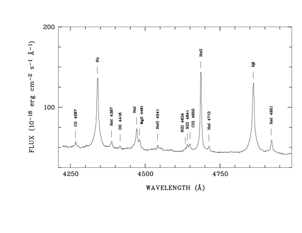
Figure 1: Orbital mean blue spectrum of QQ Vul in August 1993

3.1 Spectroscopic ephemeris of the secondary star

The orbital mean spectrum of our 1993 observations (blue spectral range) is shown in Fig. 1. The mean spectra obtained on the other occasions look very similar to that shown in the figure, although at a somewhat different brightness level. QQ Vul displays the typical features of an AM Herculis star in a high accretion state: a strong line of ionized Helium He ii $\lambda$4686, an inverted Balmer decrement, asymmetric variable lines with line wings extending to $\sim$2000 km s^-1, and a pronounced Bowen blend of Ciii/Niii-lines between 4635 and 4650 Å.

Individual emission lines consist of several components with different radial velocity amplitudes and different brightness variations. To give an example we show in Fig.2 a grey-scale representation of the phase-folded, continuum-subtracted trailed spectrogram of the He ii $\lambda$4686-line (1991 observations). The ephemeris used for phase-binning is that given in Eq. 1. The trailed blue emission line spectrogram is shown together with a trailed, continuum-subtracted spectrogram of the Na i absorption line doublet recorded simultaneously. These red spectra are fully analysed in the accompanying Paper 1 and are shown here to facilitate the interpretation of the blue spectra.

The profile of the He-line generally shows great similarity to those displayed in HU Aqr in its high accretion state (Schwope et al. 1997). The most pronounced feature is a narrow emission line (NEL) with rather low velocity amplitude. It moves parallel to the Na absorption lines, while its brightness is anticorrelated with those of the absorption lines. The latter are bright at inferior conjunction (blue to red zero crossing of the lines), the NEL is bright at superior conjunction. The NEL clearly has a much lower radial velocity amplitude than the absorption lines. Both the different brightness variation and the different radial velocity amplitude suggest that the two spectral features originate mainly from opposite hemispheres of the secondary star. This is demonstrated clearly by a combined Doppler map of both lines shown in Fig. 3. The underlying broader features in the He ii emission line complex with higher radial velocity amplitudes must then have their origin somewhere in the accretion stream. They will be investigated in section 3.3.4. Here we concentrate on the narrow emission line which obviously originates somewhere on the donor star.

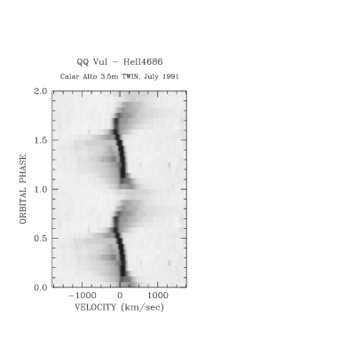
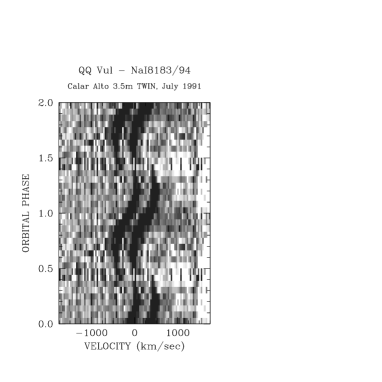
Figure 2: Trailed spectrograms of the simultaneously recorded He ii $\lambda$4686 emission and Na i $\lambda\lambda$8183/94 absorption lines of QQ Vul (1991 observations). The original spectra were continuum-subtracted and phase-folded according to the final ephemeris of Eq. 1. All data are shown twice for clarity

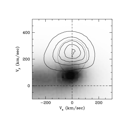
Figure 3: Doppler image (MEM-reconstruction) of the He ii emission and the Na i absorption lines recorded simultaneously in 1991. The Doppler image of Na i is shown as contourplot with iso-intensity lines at 20, 40, 60, 80 and 98% of the maximum intensity. The Doppler map of He ii is shown as a grey-scale image with dynamic range between 0 and 90% of maximum intensity. The overlay gives the size of a Roche lobe for a mass ratio $Q=1.75$, the $\times$ marks the adopted centre of mass of the secondary star.

We cannot confirm the finding by McCarthy et al. (1986) of a stationary narrow emission component at a velocity of $\sim$500 km s^-1.

The He ii $\lambda$4686 emission lines in all our spectra obtained during different years were fitted by two or three Gaussians in order to separate the NEL from the stream emission. This was unequivocally possible only in the phase interval $0.25-0.60$, at other phases the NEL is too faint to be clearly detected or strongly blended with another relatively sharp underlying component (around phases $\sim$0.2 and $\sim$0.7). The centroid positions of the NEL were then fitted assuming a circular orbit velocity equation $v=\gamma+K\sin 2\pi(t-t_{0})/P$, with fixed period $P$.

Table 3: Fit parameters for sine fits to the He ii  narrow emission and the Na i absorption lines

Year	Cycle	$\gamma$		$K$		$t_{0}$		$O-C$
		km s-1		km s-1		HJDa		daysb
HeII narrow emission line
1986	$-11183$	$-8$$\pm$	$11$	$118$$\pm$	$11$	6718.	4720(20)	$-7$
1988	$-7266$	$-66$$\pm$	$12$	$144$$\pm$	$13$	7323.	7330(30)	$+51$
1991	$0$	$-13$$\pm$	$5$	$116$$\pm$	$6$	8446.	4767(31)	$+57$
1993	$5035$	$2$$\pm$	$8$	$111$$\pm$	$5$	9224.	4817(19)	$+19$
NaI absorption line
1985	$-14396$	$17$$\pm$	$23$	$209$$\pm$	$28$	6222.	0000(30)	$+5$
1991	$0$	$-3$$\pm$	$6$	$271$$\pm$	$8$	8446.	47042(62)	$-6$
1993	$5028$	$18$$\pm$	$7$	$228$$\pm$	$10$	9223.	3982(11)	$+1$
${}^{a}+$244 0000
${}^{b}\times 10^{-4}$

Similarly, the Na i absorption lines were fitted by a double Gaussian with a fixed peak separation and the same line widths. Again the resulting radial velocities were fitted by a circular orbit velocity equation and the values given in Paper 1 are quoted here. Ellipsoidal fits gave smaller residuals than the straight sine fits (Paper 1); the influence on the times $t_{0}$ of zero crossing, however, is negligible. We compile the results for all fit-parameters in Table 3 and include also those found in the literature (Mukai & Charles 1987, Na i measurement).

Linear regressions for the times of blue-to-red zero crossing were performed for the emission and the absorption features. They yielded identical results within the errors. The weighted linear regression for the combined Na i- and He ii-lines yields

$$T_{0}\mbox{(HJD)} = 244\,8446.47105+E\times 0.15452011$$

$$\phantom{244\,8446.47}(48)\hskip 59.0pt(11)$$

(the numbers in brackets are the uncertainties in the last digits). The epochs defined by integer numbers of $E$ are regarded as epochs of inferior conjunction of the secondary star in QQ Vul. All phases in both papers refer to the ephemeris of Eq. 1. The residuals of several features recorded around the orbital cycle, such as radial velocity zero crossings, centres of linear polarization pulses, X-ray absorption dips, are plotted in Fig. 4 with respect to Eq. 1. This diagram shows the good agreement of the narrow emission-line zero crossings with Na i absorption-line zero crossings. It shows furthermore that the ‘peak 2’ component of Mukai et al. (1987) which was suspected to originate from the secondary star has nothing in common with the narrow emission line from the companion investigated here. In addition it shows the variability of the phase of the X-ray absorption dip (the bars in the diagram denote the duration of that feature, not the phase error) and it shows finally, that the linear polarisation pulse appears at random phase between phase 0.33 and 0.50 and cannot be used in order to derive the orbital period.

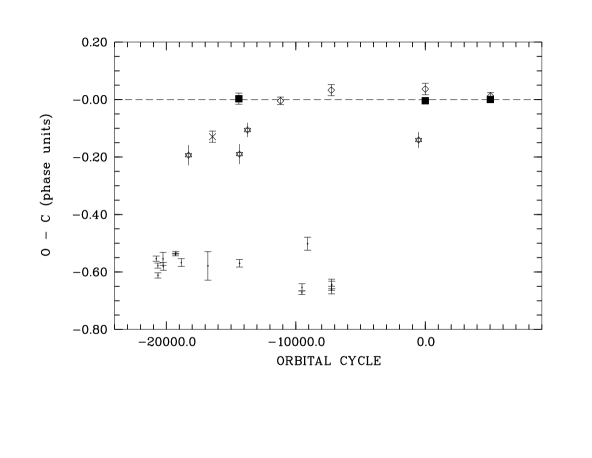
Figure 4: Residuals of events around the binary orbit in QQ Vul with respect to the linear ephemeris of Eq. 1. Meaning of symbols: $\diamond$ – NEL blue-to-red zero crossing; filled square – Nai blue-to-red zero crossing; $\times$ – Mukai et al. peak ‘2’ component; $\cdot$ – linear polarisation pulses; $\ast$ – X-ray absorption dips.

3.2 Analysis of polarimetric observations

3.2.1 Overall characteristics of the light and polarization curves

Figure 5: Phase-averaged light and polarization curves of QQ Vul obtained in 1985 and 1988 in white light. Shown are from top to bottom the brightness (in arbitrary units), the degree of circular and linear polarization and the polarization angle. The data are shown twice for clarity. Phase zero is the inferior conjunction of the secondary star (ephemeris given in Eq. 1).

In Fig. 5 we show phase-averaged light and polarization curves with full phase coverage obtained in 1985 and 1988 in white light. All data were phase-folded and averaged using the ephemeris derived in Sect. 3.1, where phase zero indicates inferior conjunction of the secondary star. The data obtained in 1987 are very similar to those obtained one year later, but with poorer signal-to-noise. These data are therefore not discussed separately.

The 1985 data are quite similar to those published recently by Cropper (1998) and to those by Nousek et al. (1984) but show some striking differences from the 1988 data with respect to the shape of the curves and the phasing of individual features.

The light curve at all three epochs is double-humped with primary and secondary minima separated by a half orbital cycle and the primary minimum centred around $\phi_{\rm spec}\simeq 0.9$. In June 1985, maximum light occurred at the phase of the second hump whereas in all later data the first hump was stronger (see Fig. 11). The phasing of the light curve does not show dramatic changes between 1985 and 1988, quite unlike the circular and linear polarisation curves which do.

Circular polarization is almost always negative with short excursions at low level towards positive values somewhere in the phase interval $\phi_{\rm spec}=0.30-0.55$, and shows a pronounced depression at phase $\phi_{\rm spec}=0.80$ and $\phi_{\rm spec}=0.95$ in 1985 and 1988, respectively.

Linear polarization is always low, i.e. below 2–3%. The curves show one distinct linear polarization maximum (pulse) per orbital cycle. It is centred at phase $\phi_{\rm spec}\simeq 0.42$ in 1985, and marks the end of the phase interval of vanishing circular polarization in that year. In 1988, the pulse occurs at $\phi_{\rm spec}\simeq 0.35$, and marks the start of the interval of positive (or vanishing) circular polarization. Not so easily recognizable in the phase-averaged representation of Fig. 5 is a second fainter linear polarization pulse at $\phi_{\rm spec}=0.57$ observed in 1988 which coincides with a second circular polarization zero crossing. The linear polarization angle displays a large scatter in 1985, whereas the variation is much simpler in 1988. Meggitt & Wickramasinghe (1982) derived a simple relation for the derivative of the polarization angle at the time of the polarization pulse for the case of a point-like emission region, $\dot{\psi}_{\rm p}=\cos{i}$. The observed data do not allow us to determine a unique value for $\dot{\psi}_{\rm p}$ in 1985, contrary to 1988 where $i\simeq 60\degr$. The fact that the value of $\dot{\psi}_{\rm p}$ changes during the pulse in the 1985 observation means that the emission region must have had a more complicated shape on that occasion compared with the 1988 observation.

The optical light and polarization curves of AM Herculis binaries are modulated by cyclotron beaming, eclipses by the secondary star and the accretion stream, and self-eclipses of the accretion region by the white dwarf itself. X-ray observations on different occasions using the EXOSAT satellite have shown that there is no eclipse by the secondary star (Osborne et al. 1987). The polarimetric data in 1985 were taken simultaneously with an EXOSAT observation. The combined data show clearly that the depression in the circular polarization at phase $\phi_{\rm spec}\simeq 0.8$ is due to an obscuration of the accretion spot by the intervening accretion stream. It is that part of the stream which is magnetically coupled and lifted out of the orbital plane. As has been pointed out by Cropper (1998), this requires the orbital inclination $i$ to be larger than the colatitude of the accretion spot $\delta_{\rm s}$ (measured with respect to the rotation axis).

Around the phase of the X-ray and circular polarization dip the observer looks almost directly onto the accretion region (minimum angle between the line of sight and the surface normal at the accretion spot). At this viewing angle the optical flux and the circular polarization are reduced due to strong cyclotron beaming. The primary optical minimum (and circular polarization dip) is, therefore, caused by the combination of depolarization/absorption in the stream and cyclotron beaming.

The secondary optical minimum at phase $\phi_{\rm spec}\simeq 0.4$ marks the phase when the accretion spot is at the limb of the white dwarf. Its phasing coincides with a sign reversal of circular polarisation and the occurrence of linear polarisation pulses. On the basis of those clues, we interpret the pronounced secondary minimum in the light curve seen in 1988, which is even more pronounced in the 1991 and 1993 data (see Fig. 11), as caused by a partial self-eclipse of an extended accretion region. The EXOSAT X-ray light curve of September 14/15 1985 shows a broad primary minimum at that phase which is being interpreted by us as the combined effect of the partial self-eclipse and foreshortening of an extended accretion spot.

Figure 6: Variation of the linear polarization position angle in the 1988 data shown together with some models. The three model curves correspond to $i=70\degr$ (short-dashed line), 60°(solid line), and 50°(long-dashed line) and length of self-eclipse of 0.21 phase units.

3.2.2 Modelling the 1988 polarimetry

To determine the accretion geometry of QQ Vul we take the simple view of a pointlike accretion region in a dipolar geometry. A simplified sketch of the geometry is shown in Fig. 7. Three vectors play an important role, the magnetic axis $\vec{\mu}$, the surface normal in the accretion spot $\vec{s}$, and the field in the spot $\vec{f}$. All vectors are shown projected onto an $x^{\prime}-z$ plane centred on the white dwarf with $z$ being parallel to the rotation axis. For an analogous representation of the geometry see e.g. Cropper (1989). The stellar co-latitudes of the dipolar axis, the spot and the field therein are measured with respect to the rotation axis and designated $\delta$ with the corresponding subscripts $\mu,s,f$. Similarly, the azimuths, $\chi$, of these vectors are measured with respect to the line joining both stars. Conventionally the accretion stream in our geometry is deflected towards negative azimuth. Below we will discuss also the azimuth of the threading region, $\chi_{\rm th}$ (Fig. 8), which is defined in the same reference frame.

Previous determinations of the accretion geometry based on polarimetry were published by Nousek et al. (1984) and Cropper (1998). Nousek et al. used a point-like accretion spot and derived a stellar latitude of the accreting magnetic pole in the range $27\degr-10\degr$, and an orbital inclination of $i=46\degr-74\degr$. Cropper (1998) investigated extended accretion arcs with constant temperature, magnetic field and density, and derived $i\simeq 40\degr-50\degr$ and a co-latitude of the magnetic dipolar axis $\delta_{\mu}\simeq 10\degr$.

The markedly different yet simpler behaviour seen in the 1988 data relative to all previous observations, called for a redetermination of the accretion geometry. Furthermore, with our extended data set, it is possible to find a solution that can encompass the results from both polarimetry and Doppler tomography. Previous analyses also lacked an absolute reference in the binary frame. We do not attempt to perform a least-squares fit of the polarimetric data, instead we try to globally optimize the model (including polarimetry, X-ray photometry and Doppler tomography). Cropper (1998), although using a more sophisticated model which accounts for an extended accretion arc, found a full inversion of the data (as in Potter, Hakala & Cropper 1987) objectively inefficacious and also only globally optimized his model.

Figure 7: Sketch of the dipolar geometry at the white dwarf surface. Shown are a cut through the white dwarf and a single dipolar field line projected on an appropriately rotated $x^{\prime}-z$ plane. Also shown are vectors indicating the orientation of the dipolar axis $\vec{\mu}$, of the surface normal in the accretion spot $\vec{s}$, and of the magnetic field line in the accretion spot $\vec{f}$, the latter being tangent to the field line at the footpoint. In a dipolar geometry $\vec{s}$ and $\vec{f}$ are always different.

The following observed features are used for an estimate of the geometry: the length of the self-eclipse $\Delta\phi_{\rm self}$, the variation of the polarization angle, and the phase of the circular polarization dip. Variation of the dipolar axis $\vec{\mu}$, the inclination $i$, and the coupling radius then predicts a different run of the polarization angle. By integrating the equation of motion for one particle with given mass ratio $Q$, one can also predict its velocity pattern in the $(v_{x},v_{y})$-plane (a schematic Doppler map) when projected with the assumed orbital inclination. The resulting image can then be compared with the observed Doppler maps (Sect. 3.3.4) thus constraining the azimuth $\delta_{\rm th}$ of the threading region. A solution is accepted if the predicted tomogram and the predicted curve of polarization angle are globally optimized and the phase of the X-ray/circular polarization dip is reflected well.

The separation between the linear polarization pulses is 0.24 phase units. The sign reversals of the circular polarization are separated by 0.18 phase units. For our estimate we use the mean of both values, $\Delta\phi_{\rm self}=0.21$. Both features are, in principle, measures of the same event, namely when the line of sight is perpendicular to $\vec{f}$. The length of the self-eclipse of the accretion spot is shorter than this phase interval. The inclination is approximately 60°, as suggested by the slope $\dot{\psi}_{\rm p}$ of the polarization angle during the pulse (Fig. 6). The values of $i$ and $\Delta\phi_{\rm self}$ constrain the possible values of the colatitude $\delta_{\rm f}$ of the field line to a certain range (see Brainerd & Lamb, 1985, for technical details). The dip is centred at $\phi_{\rm spec}=0.95$, corresponding to an azimuth of about $-20\degr$.

Model curves for the polarization angle for the acceptable range of inclination angles, $i=50\degr-70\degr$, are shown in Fig. 6 together with the 1988 data. Deviations between model and observation in the phase interval 0.8 – 1.1 should not be taken seriously, since this is the phase of depolarization in the stream and low intensity due to cyclotron beaming. The adopted values of the magnetic colatitude for the three model curves are $\delta_{\rm f}=47\degr$, $38\degr$ and $27\degr$ for $i=50\degr$, $60\degr$ and $70\degr$, respectively.

Figure 8: Model for the coupling of the accretion stream as seen by a hypothetical observer located at the white dwarf. The big circle represents the secondary star. The adopted orientation of the dipole $\vec{\mu}$ is given by its azimuth $\chi_{\mu}=-50\degr$ and its colatitude $\delta_{\mu}=23\degr$.

A globally optimised fit taking into account the different observational quantities was achieved with the following system parameters: mass ratio $Q=M_{1}/M_{2}=1.75$, inclination $i=60\degr$, orientation of the dipole axis $\delta_{\mu}=23\degr$ and $\chi_{\mu}=-50\degr$, azimuth of the threading region $\chi_{\rm th}=-20\degr$. With these parameters the accretion spot emerges at $\delta_{s}=33\degr$ and $\chi_{s}=-40\degr$, and the field line within the spot has $\delta_{f}=36\degr$ and $\chi_{f}=-37\degr$. In Fig. 8 a series of field lines around this particular one is shown as seen from the white dwarf. An observer viewing the binary at inclination $i$ would be rotating along a line of constant latitude $l=90\degr-i$. Hence, the figure illustrates that the line of sight for a likely inclination of about $60\degr$ crosses the stream between $\chi=-17\degr\mathrm{\dots}-32\degr$, which corresponds to orbital phase $\phi_{\rm spec}=0.91\mathrm{\dots}0.95$. At that phase the X-ray absorption dip was observed in the September 1985 data. The model thus reproduces the observed motion of the polarization angle, the observed phase of the X-ray/circular polarization dip, and it reflects the main features of the Doppler tomograms (see Sect. 3.3.4).

Based on the analysis of the 1988 polarimetry we do not claim an accuracy of the orbital inclination $i$ and the co-latitude $\delta_{f}$ better than $10\degr$. One should bear in mind, however, that these two quantities cannot be varied independently, they communicate with each other via $\Delta\phi_{\rm self}$. A higher inclination requires a lower co-latitude of the field $\delta_{f}$ and of the spot $\delta_{s}$. We note in particular that our estimate of $i$ based on polarimetry is in full agreement with the results of Paper 1, $i=65\degr$, using high-resolution spectroscopy of the infrared Na lines. It is also in agreement with the analysis in Nousek et al. (1984), which is worth mentioning since their data look quite different. The somewhat lower values favoured by Cropper (1988), $i=40\degr-50\degr$, are likely to be caused by the large scatter of the polarization angle in his data which indicates a more complicated accretion geometry in 1983 – 1985.

Our results imply certain values of the azimuth and co-latitude of the accretion spot, which are in good agreement with X-ray photometry (not used for the determination of the geometry so far). The value of $\chi_{s}=-40\degr$ predicts a minimum in the X-ray flux at phase 0.39 due to projection effects. Indeed, this is exactly the phase where the broad X-ray minimum occurred in the EXOSAT data taken in September 1985 (Osborne et al. 1987). Although the X-ray and our polarimetric observations were not carried out simultaneously, the simple shape of the X-ray light curve in 1985 and the simple polarimetric behaviour of QQ Vul seen in 1988 are suggestive of a similar accretion geometry. On the other hand, our parameter combination of $i$ and $\delta_{s}$ predicts a complete self-eclipse of the point-like accretion region at that phase, $i+\delta_{s}=93\degr>90\degr$, which is not observed. However, this does not necessarily imply that the model is incorrect. For one, the uncertainties associated with our derived values are larger than $5\degr$. More importantly, the accretion region is likely to be extended.

3.2.3 Changes of the accretion geometry

Up to this point, we have considered and modelled only the 1988 observations. The shift of the X-ray absorption dip towards earlier phases in June 1985 and October 1983, when the X-ray light curve had a complex shape, suggests that threading of the stream occurs further downstream, i.e. farther away from the $L_{1}$–point at an azimuth of $\chi_{\rm th}\sim-70\degr$. The X-ray lightcurve of June 1985, on the other hand, shows a completely different shape from the September 1985 data, which cannot be explained by a simple migration of the accretion spot towards a different azimuth. The fact that phasing of the X-ray maximum in June 1985 occurs exactly at the phase of minimum flux in the light curve taken three months later suggests the presence of a second active accretion region on the opposite hemisphere (Osborne et al. 1987). The corresponding cyclotron emission from the second region must affect the polarization measurements and probably distorts the simple variation of the polarization angle seen in 1988, which likely represents a one-pole accretion mode. This was already pointed out by Cropper (1998) who also detected a second polarization pulse at optical minimum phase. We confirm this likely presence of a second accretion region based on our observation of enhanced linear polarization at $\phi_{\rm spec}=0.0$ in our 1985 data.

3.3 Analysis of the emission lines

3.3.1 Origin of the narrow emission lines

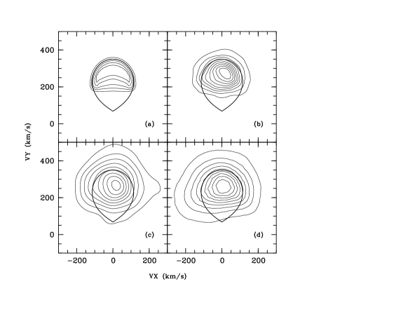
Figure 9: Numerical experiments showing the effects of noise and sampling on the reconstructed Roche lobe. The input Roche lobe used for generation of synthetic spectra is shown in each panel. (a) Reconstruction without noise, infinite velocity resolution and velocity sampling 12 km s^-1, phase sampling 0.00556; (b) reconstruction with noise at observed level, velocity resolution 80 km s^-1, phase sampling 0.0556; (c) reconstruction with noise at observed level, velocity resolution 180 km s^-1, phase sampling 0.0556; (d) reconstruction of the observed (1991) spectra. In panels (b) – (d) the isocontours represent between 10% and 90% of maximum intensity in steps of 20%. The isocontours drawn in (a) are the 20% – 80% intensity levels in steps of 20% with an additional contour at 90%.

Our initial analysis of the simultaneously recorded spectrograms of the He ii emission and the Na i absorption lines in Sect. 3.1 based on radial velocity fits suggests that the NEL and the absorption lines originate on opposite hemispheres of the secondary star. This impression is supported by a combined Doppler tomogram of both lines (Fig. 3) which was constructed using MEM-deconvolution of the trailed spectrograms. We had chosen the He ii emission line for this initial analysis because it is intrinsically the sharpest of the bright lines in the blue spectral regime. With a full width at half maximum FWHM of 1.9 Å (1991) and 2.0 Å (1993) at phase 0.5, the NEL of He ii is just resolved. The NEL components of the H-Balmer lines at the same phase have a FWHM of 3.7 Å, those of He i have 2.5 – 4 Å. The NEL of Mg ii $\lambda$4481 is comparable in width to that in He ii $\lambda$4686 but has a much lower flux and thus reduced signal-to-noise.

A comparison of the results from the fit to the radial velocity measurements and those from the Doppler map (Sect. 3.1) for the same data set reveals an inconsistency between the radial velocity amplitudes in the NEL. Maximum emission in the Doppler map occurs at $v=|v_{y}|\simeq 96$ km s^-1 whereas the radial velocity fit gives $v=116\pm 6$ km s^-1. We think that this inconsistency results from the reduced phase interval in which the NEL velocities can be derived with good accuracy. Thus, we will use radial velocity amplitudes derived from the Doppler maps which are based on all the data instead of a restricted data set. To compute the Doppler maps we mainly used the code of Spruit (1998).

Figure 10: Velocity ratio of the photocentres of the irradiated front- and the non-irradiated backside of the donor star due to our irradiation model compared with the observed velocity ratios of Na i absorption lines (271 km s^-1) and narrow emission lines (NEL) of different species (data from 1991 and 1993). The solid line is a spline fit through the filled dots which were computed for $i=90\degr$, the open circles were computed for $i=60\degr$ (fit indicated by dashed line).

The relatively sharp separation between emission and absorption features in the Doppler map shown in Fig. 3 requires us to address the following questions. (1) Is it possible to reconstruct the shape of the Roche lobe and thus determine the mass ratio $Q$ using Doppler maps of the Na i-lines alone? (2) Is it possible to measure the size of the Roche lobe of the secondary directly using the velocities of the illuminated and the non-illuminated hemispheres of the secondary star provided these could be unequivocally determined observationally? Answering these questions, in particular locating the $L_{1}$-point, is essential for the next section’s investigation of the accretion stream using Doppler tomography.

3.3.2 An irradiation model for the secondary star

To address both questions we computed synthetic line profiles using an illumination model of the secondary star like the one used in MR Ser and HU Aqr (Schwope et al. 1993, Schwope et al. 1997). The procedure is described in detail in Beuermann & Thomas (1990).

In brief, the irradiating source is located at $M_{1}$, it is assumed that the secondary star fills its Roche lobe, that no shielding of the secondary’s surface by the accretion stream or an accretion curtain occurs and that a sharp separation of irradiated and non-irradiated parts of the secondary exists. We assume that both emission and absorption lines originate from the photosphere, i.e. from the Roche lobe of the secondary. The shape of the Roche lobe is iterated for given $Q$. Line emission from a surface element on the irradiated secondary is taken to be proportional to the solid angle as seen from the source at $M_{1}$. Radiation is assumed to be optically thick, hence foreshortening of surface elements has to be taken into account. For the non-illuminated parts of the secondary star we assume that an absorption line is formed whose strength is proportional to the size of the surface element and also take foreshortening of the individual element into account. Emission and absorption line profiles are synthesized using the full Roche geometry. Since the spread of the radial velocity over the secondary’s surface is of the order of several hundred km s^-1, we regard velocity broadening as the only broadening mechanism of spectral lines. In order to transform velocities from dimensionless binary coordinates into the observer’s frame, we adopt the mass-radius relation by Neece (1984) for the secondary star. The often used empirical relation by Caillault & Patterson (1990) gives slightly different results (see below).

As mentioned above, our model does not take into account any kind of shielding of the secondary star by e.g. an accretion curtain. This was present at some occasions in AM Her and HU Aqr (Davey & Smith 1996, Schwope et al. 1997) and became obvious in these stars by a prominent left/right asymmetry of the Doppler maps. Such an obvious asymmetry is not present in the combined He/Na Doppler map of QQ Vul, the centres of light of both species lie at $v_{x}=0$ km s^-1 (Fig. 3), i.e. indicating no or far less shielding in 1991 than in 1993. Shielding was present in 1993 (cf. Paper 1), with the effect that the radial velocity curve of Na i had a higher ellipticity, yet smaller amplitude.

In order to answer question (1) we computed absorption line profiles with the same spectral resolution, orbital phase sampling and noise level as our 1991 observations. In Fig. 9 we compare reconstructions of data with (a) infinite resolution and S/N, (b) resolution, sampling and noise as in 1991 ($v_{\rm FWHM}=80$ km s^-1 measured using arc lines), (c) sampling and noise as before but degraded resolution ($v_{\rm FWHM}=180$ km s^-1) and (d) with a reconstruction of the observed data. The Roche lobe used for generation of the data is shown in each panel.

From that exercise we learned (panel a) that it is possible to reconstruct the original shape of the non-irradiated hemisphere of the companion star using high-quality data (high resolution, low noise), not a big surprise. The reconstruction shown in panel (b), which uses data of same quality as the observed data appears somewhat smeared. This map has already lost the arc shape of the inner contours of the reconstruction in panel (a).

Due to the limited resolution of the data, the contours extend into the nominally dark, front-side hemisphere of the star. The whole map has a smaller FWHM than the reconstruction of the observed data (panel d). In order to match the FWHM of the map in panel (d) we had to degrade the resolution in our simulation to values as high as $\Delta v=180$ km s^-1. The resulting map (c) is almost rotationally symmetric and no longer displays a half star as all other maps do. The high degree of similarity between maps (b) and (d) suggest that the Na i absorption almost entirely originates from the non-irradiated hemisphere of the companion star and that the size of the Roche lobe chosen for the simulations is a fairly good representation of the true size. Variation of $Q$ increases the size and shifts the lobe along the $v_{y}$-axis and makes the fit worse.

Our guess is that the observed map is disturbed by some effect and is, therefore, not as sharply reconstructed as the simulated one. For example, emission from the nearby He ii $\lambda$8236 line and the corresponding curved continuum could easily contaminate the absorption lines. The range of $Q$, which gave acceptable fits (by eye) to the location and curvature of the contours of the observed Doppler map, is $Q=1.5-2.2$ (for $i$ between 50° and 71°) with a best agreement at about $Q=1.8$.

Figure 10 addresses question 2. We attempt to (further) constrain the mass ratio using the velocity ratio of the photocentres of the illuminated and non-illuminated hemispheres of the secondary star. Synthetic spectra computed for different mass ratio $Q$ and orbital inclination $i$ were used. The inclination only has a small effect on the velocity ratio. Theoretically, the velocity ratio $v_{\rm b}/v_{\rm f}$ is a steep function of $Q$. This – in principle – offers the opportunity to measure the size of the Roche lobe by determining the velocities of the photocentres. We assume that, observationally, the velocity of the non-irradiated side of the secondary star is $v_{b}=271$ km s^-1, the largest velocity amplitude of the Na i lines measured so far (1991 data). Above we have argued that the Doppler map is consistent with a complete depletion of the irradiated front side of Na absorption. Incomplete Na depletion would mean that the true $v_{b}$ would be larger and the derived mass ratio be smaller.

Using all NEL’s radial velocity amplitudes with estimated uncertainties better than 10 km s^-1 as potential tracers of $v_{f}$, observed ratios $v_{b}/v_{f}$ were computed. These ratios, shown as dotted lines in Fig. 10 are highly dispersed, from 85 km s^-1 for Hei 4471 in 1993 to 135 km s^-1 for Caii in 1991, and do not allow us to constrain the mass ratio better than when using the Na i lines alone (see above and Paper 1).

For $Q\simeq 1.85$ and $i=65\degr$ (Paper 1), the predicted velocity $v_{f}$ is $115-125$ km s^-1, that of the $L_{1}$-point is $v_{\rm L1}\simeq 75-80$ km s^-1, $v_{b}/v_{f}=2.36-2.17$. For these parameters the H-Balmer lines are apparently the most suitable tracers of $v_{f}$. The Ca and Paschen lines are compatible with this solution within the accuracy of our velocity determination, while the He ii lines display too low velocities, i.e. they originate closer to the $L_{1}$-point. Obviously these lines are formed in an extended quasi-chromosphere located above the photosphere. The He ionizing radiation is not able to reach the whole geometrically allowed hemisphere of the secondary. The data presented here are thus able to resolve (although marginally) these different layers. A quantitative understanding of the formation of the emission lines requires detailed modelling of non-isotropically X-ray irradiated photospheres of late-type stars, a project within reach of current models (e.g. Hauschildt, Baron & Allard 1997), but not yet undertaken.

3.3.3 Multi-epoch line flux variations

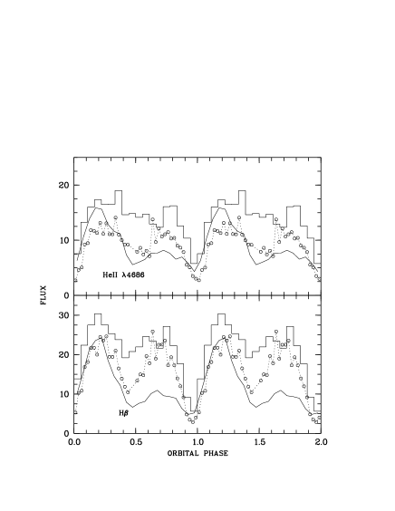
Figure 11: (a, left) Continuum and emission line light curves (He ii $\lambda$4686, H$\beta$) of QQ Vul in 1986 (solid lines), 1991 (histograms), and 1993 (circles). The continuum flux is the wavelength-averaged flux over the line-free wavelength interval indicated in the top panel in units of 10^-16 erg cm^-2 s^-1 Å^-1. Line flux is the integrated line flux in units of 10^-14 erg cm^-2 s^-1. (b, right) Emission line light curves after subtraction of the approximated contribution of reprocessed emission from the secondary star thus leaving emission only from the accretion stream.

For the analysis of emission lines originating from the stream, we make use of emission line light curves and Doppler maps, shown in Figs. 11 and 12. The emission line light curves are based on the integrated line profiles of the trailed spectrograms shown in Fig. 12. We approximately removed the contribution of the NEL, which does not originate from the stream, by measuring its flux at phase $\phi_{\rm spec}=0.5$, adapting a simulated emission line light curve to that level and subtracting it from the total flux. These NEL-free light curves are also shown in Fig. 11. For comparison, continuum light curves extracted from a line-free region between the two emission lines H$\beta$ and He ii $\lambda$4686  are also shown.

The continuum light curves are all similar in shape displaying a double-humped structure with the primary minimum centred on $\phi_{\rm spec}\simeq 0.95$ in 1991 and 1993 and probably somewhat earlier, $\phi_{\rm spec}\simeq 0.92$ in 1986. As discussed in Sect. 3.2 this minimum is caused by cyclotron beaming and the small shift of minimum phase at the different epochs indicates a possible azimuthal shift of the emission region.

The emission line light curves are also double humped with intensity maxima at phase 0.2 and 0.7. This behaviour is more pronounced in H$\beta$ than in He ii and more obvious after subtraction of the NEL, which peaks at $\phi_{\rm spec}=0.5$. Pronounced minima occur in the phase interval 0.92 – 1.00, the minima in H$\beta$ generally occur earlier by $\sim 0.03-0.05$ phase units at all epochs. The minima in both lines occurred earlier in 1986 than in 1993. The light curves in 1986 are highly asymmetric with a pronounced first maximum which is more than double the height of the second one. All these observed properties are suggestive of optically thick radiation in the accretion stream, with the stream having a higher thickness in 1986 than at the two other epochs.

3.3.4 Multi-epoch trailed spectrograms and Doppler maps of He ii $\lambda$4686

Also the trailed spectrograms and the Doppler maps are markedly variable between the three epochs. We show in Fig. 12 the trails and maps of He ii $\lambda$4686. The data of the other emission lines look very similar as far as the velocity pattern (though not the brightness pattern) is concerned. Looking first at the trailed spectra, the narrow emission line (NEL) is the most obvious and the most pronounced feature in all three observations. The underlying emission from the stream is brighter close to the NEL-emission in 1991 and 1993 than in 1986. Hence, during the two recent observations the stream was brighter in the vicinity of the inner Lagrangian point $L_{1}$ at rather lower velocities than in 1986, when stream emission was bright at higher velocities.

This is nicely illustrated too in the Doppler maps which are shown as contour plots below the trailed spectrograms in Fig. 12. Contour levels were chosen appropriately to emphasize stream emission (the inner contour corresponds to the maximum intensity level from the stream). In 1991 and 1993, there is some bright emission originating approximately at $L_{1}$ and extending down to velocities $v_{x}\sim-500$ km s^-1 at constant $v_{y}$. From there a tail stretches down to the lower left region of the maps which can be recognized at velocities as high as $(v_{x},v_{y})=(-1200,-700)$ km s^-1. Within the resolution of our data, the orientation of these high-velocity tails is the same in all maps.

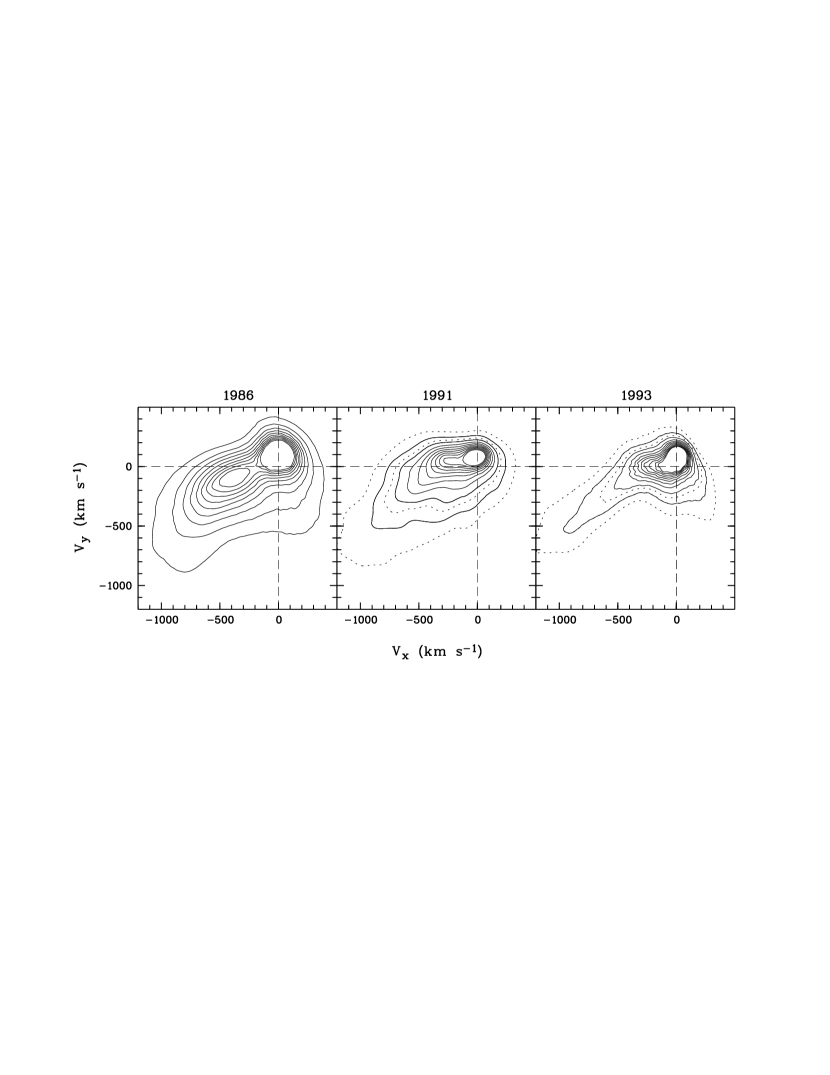
Figure 12: Trailed spectrograms (top) and MEM-reconstructed Doppler maps (bottom) of the He ii emission lines in 1986, 1991 and 1993. All spectra were continuum-subtracted and phase-averaged according to the ephemeris given in Eq. 1. The dynamic range of the grey-scale representations is between 0 and $150\times 10^{-16}$ erg cm^-2 s^-1 Å^-1, the same in each panel. Isocontour lines drawn with solid lines represent emission at 10%, 20% …90% of maximum emission originating from the accretion stream. For the 1991, and 1993 tomograms contours at the 5% and 15% level are shown in addition drawn with dashed lines.

The initial ridge of emission between $L_{1}$ and $(v_{x},v_{y})\sim(-400,50)$ km s^-1 can be tentatively identified with emission originating from the ballistic stream, as seen as prominent features in HU Aqr and UZ For (Schwope et al. 1997, 1999). There are, however, some problems with this interpretation, since this ridge shows a displacement by $\Delta v_{y}\simeq 45$ km s^-1 between 1991 and 1993. If it were a purely ballistic stream, it would be fixed in the binary and always appear at the same $v_{y}$–velocity. In the following, we will use the term ‘ballistic’ stream for the bright ridge of emission connected to the secondary star seen in the 1991 and 1993 tomograms, although it might not appear at a ballistic velocity at all.

Figure 13: Model of the accretion stream in Doppler coordinates. The adopted orientation of the dipole $\vec{\mu}$ is given by its azimuth $\chi_{\mu}=-50\degr$ and its colatitude $\delta_{\mu}=23\degr$, the same as in Fig. 8. With this geometry the ballistic part of the stream is truncated at $v_{x}\simeq-500$ km s^-1. The magnetically controlled part of the flow appears in the lower left quadrant. The straight line at the centre of the bundle of trajectories indicates the location of the observed stream.

We determined the location of the ballistic stream by fitting a Gaussian curve to the Doppler maps at $v_{x}=-250$ km s^-1. Maximum emission ocurred at $v_{y}\simeq 45$ km s^-1 in 1991 and at $v_{y}\simeq 0$ km s^-1 in 1993. For a first-order estimate we set the $v_{y}$-velocities at $L_{1}$ and at $v_{x}=-250$ km s^-1 to be the same. For our best guess of $Q$ and $i$, the projected velocity $v_{y}$ at $L_{1}$ is $75-80$ km s^-1 (see above). Only for the lower limit value $Q=1.5$, $i=70\degr$, is the projected $v_{y}=51$ km s^-1 as low as observed in 1991. Hence, on both occasions (1991 likely, 1993 definitely), the observed ballistic stream appears at smaller velocities $v_{y}$ than predicted by a single-particle trajectory for the likely parameter combination of $i$ and $Q$.

Emission which could be apparently associated to the ballistic stream was almost completely absent in 1986. At that epoch a bright spot of emission centred on $(v_{x},v_{y})\simeq(-380,-100)$ km s^-1 emerged instead.

As a first step to gain a quantitative understanding of the location and extent of the different parts of the stream in the magnetosphere, we have computed models for the accretion stream, representing it by a single-particle trajectory under gravitational and centrifugal influence. We accounted for the pull of the magnetic field on the partly ionized stream by a magnetic drag force decreasing exponentially as a function of radius. This additional drag redirects the trajectory in a small region in physical space. It initially follows a ballistic path and then follows a dipolar field line. The velocity component along the field is conserved in our computation when the particle latches onto the field line. Depending on the orientation of the magnetic field in the threading region, the re-direction of the stream may result in a rather large step in velocity space $(v_{x},v_{y})$ (see Schwope et al. 1997 for further details).

A model which accounts for most of the observed features of the 1991 and 1993 tomograms of He ii is shown in Fig. 13. We simulated several different trajectories coupling at different radii by varying the magnetic field strength, which appears as a dimensionless tuning parameter in our calculations. The trajectories shown in Fig. 13 in velocity space are the same as those shown in Fig. 8 in real space. The smaller the assumed value of the field strength, the longer the particle remains on the ballistic trajectory (coupling at larger azimuth) and the higher the velocity at the threading point becomes. Observationally, the ballistic part of the accretion stream can be followed down to $v_{x}\simeq-500$ km s^-1. It is perhaps a bit more elongated in 1991 than in 1993, but this is difficult to state exactly, because the Doppler map of 1991 has a poorer velocity resolution. A velocity of $v_{x}\simeq-500$ km s^-1 on the ballistic stream corresponds to an azimuth of the coupling region of about $-25\degr$. Coupling may – in principle – occur all along the ballistic stream between the $L_{1}$ point and that azimuth. The orientation of the axis of the magnetic field was chosen in accord with polarimetry (Sect. 3.2). With the chosen field geometry the magnetically funnelled part of the trajectories stretches along a more or less straight line in the lower left quadrant of the velocity plane, almost exactly along the observed high-velocity ridge in the Doppler maps (indicated by a straight line in Fig. 13).

This simple model cannot account for the observed displacement towards smaller $v_{y}$-velocities of the ‘ballistic’ stream with respect to the single-particle trajectory. One possible explanation for this displacement is that a proper ballistic stream (not influenced by the magnetic field) exists but that the observed emission is dominated by matter with slightly changed velocity (matter in the process of getting coupled). Another possibility has recently been worked out by Sohl & Wynn (1999) who treated the accretion flow as a number of diamagnetic blobs which independently interact with the magnetosphere of the primary. This model predicts blob trajectories differing from single-particle trajectories and might be applicable to QQ Vul.

The apparent absence of a ballistic stream in 1986 and the occurrence of the bright spot at $(v_{x},v_{y})\simeq(-380,-100)$ km s^-1 remains unexplained so far. There might be two explanations for the missing ballistic stream: either matter couples on the field directly at $L_{1}$ or the stream was outshone by other emission components and therefore not recognizable at the phase and spectral resolution of our observations. We investigated the first possibility by tuning the magnetic field strength in our models to high values (which mimics low accretion rates), so that no ballistic stream was formed. We then used different orientations of the dipolar axis in order to check whether the trajectory runs through the observed bright spot down to the lower left quadrant in the $(v_{x},v_{y})$ plane. Azimuth and latitude of the magnetic axis were varied over large ranges but no solution was found. We conclude that the resolution of the 1986 data and the brightness of the other components prevented us from detecting emission from the ballistic stream.

3.3.5 A simple model for the emission line light curves

Support for the view that the bulk of matter does not couple at $L_{1}$ but somewhere downstream comes from some numerical experiments which were performed to reach a basic understanding of the emission line light curves. A single-particle trajectory between the $L_{1}$ point, the coupling region and the white dwarf was divided in 100 parts of equal length and each element was assigned an intensity value. We allowed for two different brightness values, depending on whether the irradiated or the non-irradiated side of the stream was seen. Emission from an element was assumed to be optically thick, hence the observed brightness of an element at a given phase was the intrinsic brightness times a foreshortening factor. The brightness $b$ of the vertical stream (along the dipolar field line) was varied as a function of radius with $b\propto r^{1.5}$ starting with some initial value in the threading region. This radial dependence accounts for the shrinkage of the effectively emitting area due to the converging field lines. Light curves were computed by coadding over all visible elements at a given phase taking the full Roche geometry into account so that eclipses of parts of the stream are recognized if the inclination is high enough.

Figure 14: Model of the stream emission as function of orbital phase for the ballistic part in (a) and the magnetically funnelled part in (b).

In Fig. 14 we show the resulting model light curves for the ballistic part of the stream and the magnetically funnelled part. The central trajectory of those shown in Figs. 13 and 8 was used and a contrast of $1:0.7$ between the irradiated and non-irradiated sides of the stream was adopted. The light curves were computed for an assumed orbital inclination of 65°. Both light curves were normalized to maximum emission. Emission from the ballistic stream shows emission maxima at $\phi_{\rm spec}\simeq 0.3$ and 0.8 which is simply an expression of the deflection angle of $\sim$18° of the ballistic stream with respect to the line connecting both stars. The primary minimum at $\phi_{\rm spec}\simeq 0.02$ is caused by the combined effect of foreshortening and a partial eclipse of the stream by the secondary star.

The model light curve from the magnetically funnelled part of the stream shown in Fig. 14b is affected only by foreshortening. This causes the maxima of emission to appear at spectroscopic phases 0.2 and 0.7 and the minima at phases 0.45 and 0.95. These phases are well in agreement with the observed maxima and minima of the emission lines of Fig. 11. These phasings and the absence of pronounced stream eclipses by the secondary star are suggestive of stream emission mainly originating from the magnetic part of the stream (in 1991 and 1993) or the threading region (1986). The visual impression of the Doppler maps (1991, 1993) is in apparent contradiction to this statement, since they show emission associated with the ballistic stream as a prominent feature. We regard the contradiction as apparent only for two reasons. Firstly, as discussed above, at least part of the emission associated with the ballistic stream originates from matter which is coupled to the field and thus is expected to produce a light curve resembling that in Fig. 14. Secondly, the surface brightness distribution of a Doppler map does not reflect the brightness distribution in real space. In particular, emission at high velocities is spread over a large region in a $(v_{x},v_{y})$ diagram. The summed flux of the high surface-brightness pixels in the region defined by $(v_{x},v_{y})=(-500,-40)$ km s^-1 (lower left corner) and $(120,200)$ km s^-1 (upper right corner), i.e. including the NEL from the secondary star, contributes only to about 40% (1991) and 50% (1993) of the total intensity in the maps. Hence, low surface-brightness emission from higher velocities is dominating in the stream.

The Doppler maps indicate that we can best differentiate between emission from the ballistic and the magnetic stream at phases 0.25 and 0.75, i.e. in the direction of the $v_{x}$-axis. Projection in these directions produces a relatively sharp spectral feature of emission associated with the ballistic stream (although not as sharp as the NEL from the secondary) whereas emission from the magnetic stream will appear as a rather broad feature. Fitting the observed spectra (1991 and 1993) at these indicated phases with triple Gaussians (NEL plus medium width plus broad component) reveals that the medium width and broad base components carry almost the same flux at these phases on both occasions. If we then take into account, that even the medium width component is fed by emission from matter which has already latched onto the field it seems plausible that most of the observed line emission comes from the magnetically funnelled stream and/or matter which is in the process of becoming funnelled, and that emission from the ballistic stream plays a minor role in the formation of the emission line light curves. Hence, Doppler maps and emission line light curves tell us the same story.

4 Conclusions and outlook

Using medium- and high-spectral resolution observations with full phase coverage of the long-period AM Herculis binary QQ Vul obtained on three occasions in 1986, 1991 and 1993 and complementary polarimetry obtained between 1985 and 1988 we studied the accretion geometry in the inner and outer magnetosphere. First of all, we derived a reliable spectroscopic ephemeris for inferior conjunction of the secondary star by combining Na i photospheric absorption lines with narrow emission lines of reprocessed emission from the X-ray irradiated hemisphere, HJD($T_{0}$) $=244\,8446.4710(5)+E\times 0\aas@@fstack{d}15452011(11)$. The arrival times of linear polarization pulses show a large scatter in an $(O-C)$ diagram with respect to the new ephemeris and thus are disqualified as useful tracers of the orbital motion for the case of QQ Vul.

Analysis of the linear and circular polarization curves favour an orientation of the (dipolar) magnetic axis of $\delta_{\mu}=23\degr$ and $\chi_{\mu}=-50\degr$, and an orbital inclination between $50\degr$ and $70\degr$. The variable shape of the polarization curves, in particular the phasing of circular polarization dips, suggests that the azimuth of the coupling (threading) region undergoes significant migrations in azimuth.

The suggested orientation of the magnetic dipole and of the coupling region is in good agreement with the results inferred from Doppler tomography of bright emission lines, in particular those of He ii $\lambda$4686. These show (in 1991 and 1993) three distinct emission features: (1) the irradiated hemisphere of the secondary star, (2) emission which can be associated with the ballistic stream, and (3) emission from the magnetically funnelled stream. Emission, which apparently arises from the ballistic stream, appears at different places in the Doppler tomograms of 1991 and 1993. This suggests that it is formed by matter which is in the process of becoming threaded, in complete agreement with the emission line light curves, which show the major contribution from the magnetic part of the stream. At one occasion (1986) the Doppler maps do not reveal any emission that could be associated with the ballistic stream.

We explored whether it would be possible to use the narrow emission lines from the secondary star in combination with photospheric absorption lines to constrain the mass ratio and the orbital inclination. This was not possible in QQ Vul because the radial velocity amplitudes of different atomic species were found to be widely different. Lines from high ionization species such as He ii $\lambda$4686 originate more closely to the $L_{1}$ than a reprocessing model predicts.

The Doppler tomograms presented in this paper suggest that threading of the accretion stream (or parts of it) starts very soon or perhaps immediately after leaving the secondary star. The stream seems to be completely disrupted at an azimuth of about $-30\degr$. Future observations with higher spectral and temporal resolution of the Na i-lines (1) will allow the mass ratio to be determined with an accuracy of better than 10% by the straightforward application of Doppler tomography and (2) will reveal substructure in the Doppler maps due to e.g. star spots.

References

- [] Beardmore, A.P., Ramsay, G., Osborne, J.P., Mason, K.O., Nousek, J.A., Baluta, C., 1995, MNRAS 273, 742
- [] Beuermann, K., Thomas, H.-C., 1990, A&A 230, 326
- [] Brainerd J.J., Lamb, D.Q., 1985, In: Lamb D.Q., Patterson, J. (eds.) Proc. 7th North American Workshop on CV’s and LMXBs, Reidel, Dordrecht, p. 247
- [] Caillault, J.–P., Patterson, J., 1990, AJ 100, 825
- [] Catalán, M.S., Schwope, A.D., Smith, R.C., 1999, MNRAS, in press (Paper I)
- [] Catalán, M.S., Davey, S., Smith, R.C., Jones, D.H.P., 1996, in Cataclysmic Variables and Related Objects, Proc. IAU Coll. 158, Kluwer, Dordrecht, p. 227
- [] Cropper, M., 1989, MNRAS 236, 935
- [] Cropper, M., 1998, MNRAS 295, 353
- [] Hauschildt, P.H., Baron, E., Allard, F., 1997, ApJ 483, 390
- [] Liebert, J., Stockman, H.S., 1985, in Proc. 7th North American Workshop on CVs and LMXBs, eds. D.Q. Lamb and J. Patterson, Reidel, Dordrecht, p. 151
- [] Marsh, T.R., Horne, K., 1988, MNRAS 235, 269
- [] Meggitt, S.M.A., Wickramasinghe, D.T, 1982, MNRAS 198, 71
- [] McCarthy, P., Bowyer, S., Clarke, J.T., 1986, ApJ 311, 873
- [] Mukai, K., Charles, P.A., 1986, MNRAS 222, 1P
- [] Mukai, K., Charles, P.A., 1987, MNRAS 226, 209
- [] Mukai, K., Bonnet-Bidaud, J.-M., Charles, P.A., et al., 1986, MNRAS 221, 839
- [] Neece, G.D., 1984, ApJ 277, 738
- [] Nousek, J.A., Takalo, L.O., Schmidt, G.D., et al., 1984, ApJ 277, 682
- [] Nugent, J.J., 1983, ApJS 51, 1
- [] Osborne, J.P., Beuermann, K., Charles, P.A., Maraschi, L., Mukai, K., Treves, A., 1987, ApJ 315, L123
- [] Osborne, J.P., Bonnet-Bidaud, J.-M., Bowyer, S., et al., 1986, MNRAS 221, 823
- [] Potter, S.B., Hakala, P.J., Cropper, M., 1998, MNRAS 297, 1261
- [] Proetel, K., 1978, PhD thesis, Ruprecht-Karls-Universität, Heidelberg
- [] Schwope, A.D., Mantel, K.-H., Horne, K., 1997, A&A 319, 894
- [] Schwope, A.D., Beuermann, K., Jordan, S., Thomas, H.-C., 1993, A&A 278, 498
- [] Schwope, A.D., Beuermann, K., Buckley D.A.H., et al., 1998, ASP Conf. Ser. 137, pp. 45–59
- [] Schwope, A.D., Schwarz R., Staude A., Heerlein C., Horne K., Steeghs D., 1999, ASP Conf. Ser. 157, 71
- [] Sohl, K., Wynn, G., 1999, ASP Conf. Ser. 157, 1999
- [] Spruit, H.C., 1998, astro-ph/9806141
- [] Stahl, O., Buzzoni, B., Kraus, G., Schwarz, H., Metz, K., Roth, M., 1986, The Messenger 46, 23