The Local Ly$\alpha$ Forest. II. Distribution of
H I Absorbers, Doppler Widths, and Baryon Content

Abstract

In Paper I of this series we described observations of 15 extragalactic targets taken with the Hubble Space Telescope+GHRS+G160M grating for studies of the low-$z$ Ly$\alpha$ forest. We reported the detection of 111 Ly$\alpha$ absorbers at significance level (SL) $\geq 3\sigma$, 81 with $SL\geq 4\sigma$, in the redshift range $0.002<z<0.069$, over a total pathlength $c\Delta z=116,000$ km s^-1 ($\Delta z=0.387$). In this second paper, we evaluate the physical properties of these Ly$\alpha$ absorbers and compare them to their high-$z$ counterparts. The $SL\geq 4\sigma$ distribution of Doppler parameters is similar to that at high redshift, with $\langle$$b$$\rangle=38.0\pm 15.7$ km s^-1. The true Doppler parameter may be somewhat lower, owing to component blends and non-thermal velocities. The distribution of equivalent widths exhibits a significant break at $\mathcal{W}\leq 133$ mÅ, with an increasing number of weak absorbers (10 mÅ $<\mathcal{W}<100$ mÅ). Adopting a curve of growth with $b=25\pm 5$ km s^-1 and applying a sensitivity correction as a function of equivalent width and wavelength, we derive the distribution in column density, $N_{\rm HI}$^-1.72±0.06 for $12.5\leq\log{\left[N_{\rm HI}\right]}\leq 14.0$. We find no redshift evolution within the current sample at $z<0.07$, but we do see a significant decline in d$\mathcal{N}$/d$z$ compared to values at $z>1.6$. Similiar to the high equivalent width ($\mathcal{W}>240~{}{\rm m}\mbox{\AA}$) absorbers, the number density of low-$\mathcal{W}$ absorbers at $z$=0 is well above the extrapolation of d$\mathcal{N}$/d$z$ from $z>2$, but we observe no difference in the mean evolution of d$\mathcal{N}$/d$z$ between absorbers of high ($\mathcal{W}>240~{}{\rm m}\mbox{\AA}$) and low ($\mathcal{W}\leq 100~{}{\rm m}\mbox{\AA}$) equivalent width absorbers. While previous work has suggested slower evolution in number density of lower-$\mathcal{W}$ absorbers, our new data do not support this conclusion. A consistent evolutionary pattern is that the slowing in the evolution of the low column density clouds occurs at lower redshift than for the higher column density clouds. A $4-5\sigma$ signal in the two-point correlation function of Ly$\alpha$ absorbers for velocity separations $\Delta v\leq 150$ km s^-1 is consistent with results at high-$z$, but with somewhat greater amplitude. Applying a photoionization correction, we find that the low-$z$ Ly$\alpha$ forest may contain $\sim 20$% of the total number of baryons, with closure parameter $\Omega_{Ly\alpha}=(0.008\pm 0.001)h_{70}^{-1}$, for a standard absorber size and ionizing radiation field. Some of these clouds appear to be primordial matter, owing to the lack of detected metals (Si III) in a composite spectrum, although current limits on composite metallicity are not strong.

1 Introduction

Since the discovery of the high-redshift Ly$\alpha$ forest over 25 years ago, these abundant absorption features in the spectra of QSOs have been used as evolutionary probes of the intergalactic medium (IGM), galactic halos, large-scale structure, and chemical evolution. Absorption in the Ly$\alpha$ forest of H I (and He II) is also an important tool for studying the high-redshift universe (Miralda-Escudé & Ostriker, 1990; Shapiro, Giroux, & Babul, 1994; Fardal, Giroux, & Shull, 1998). A comparison of the H I and He II absorption lines provides constraints on the photoionizing background radiation, on the history of structure formation, and on internal conditions in the Ly$\alpha$ clouds. In the past few years, these discrete Ly$\alpha$ lines have been interpreted in the context of N-body hydrodynamical models (Cen et al., 1994; Hernquist et al., 1996; Zhang et al., 1997; Davé et al., 1999) as arising from baryon density fluctuations associated with gravitational instability during structure formation. The effects of hydrodynamic shocks, Hubble expansion, photoelectric heating by AGN, and galactic outflows and metal enrichment from early star formation must all be considered in understanding the IGM.

At high redshift, the rapid evolution in the distribution of Ly$\alpha$ absorption lines per unit redshift, $d{\cal N}/dz\propto(1+z)^{\gamma}$ ($\gamma\approx 2.5$ for $z\geq 1.6$), was consistent with a picture of these features as highly ionized “clouds” whose numbers and sizes were controlled by the evolution of the IGM pressure, the metagalactic ionizing radiation field, and galaxy formation. However, the rapid evolution of the Ly$\alpha$ forest stopped at $z<1.6$. One of the delightful spectroscopic surprises from the Hubble Space Telescope (HST) was the discovery of Ly$\alpha$ absorption lines toward the quasar 3C 273 at $z_{\rm em}=0.158$ by both the Faint Object Spectrograph (FOS, Bahcall et al., 1991) and the Goddard High Resolution Spectrograph (GHRS, Morris et al., 1991, 1993). The number of these absorbers was found to be far in excess of their expected number based upon an extrapolation from high-$z$ (see e.g. Weymann et al. (1998) and section 5 therein). This evolutionary shift is probably a result of the collapse and assembly of baryonic structures in the IGM (Davé et al., 1999) together with the decline in the intensity of the ionizing radiation field (Haardt & Madau, 1996; Shull et al., 1999b). Detailed results of the Ly$\alpha$ forest evolution in the redshift interval $0<z<1.5$ are described in the FOS Key Project papers: the three catalog papers (Bahcall et al., 1993, 1996; Jannuzi et al., 1998) and the evolutionary analysis study (Weymann et al., 1998).

However, the HST/FOS studies were primarily probes of strong Ly$\alpha$ lines with equivalent widths greater than 0.24 Å. A great deal more information about the low-$z$ IGM can be gained from studies of the more plentiful weak absorbers. Realizing the importance of spectral resolution in detecting weak Ly$\alpha$ absorbers, the Colorado group has engaged in a long-term program with the HST/GHRS, using the G160M grating at 19 km s^-1 resolution, to study the very low-redshift ($z<0.07$) Ly$\alpha$ forest. Earlier results from our study have appeared in various research papers (Stocke et al., 1995; Shull, Stocke, & Penton, 1996; Shull et al., 1998) and reviews (Shull, 1997; Shull, Penton, & Stocke, 1999a).

The current series of papers discusses our full GHRS dataset. In Paper I (Penton, Shull, & Stocke, 2000a) we described our HST/GHRS observations and catalog of Ly$\alpha$ absorbers. In Paper II (this article) we describe the physical results from our program, including information on the physical parameters and nature of the low-redshift Ly$\alpha$ forest. A discussion of the relationship between the Ly$\alpha$ absorbers discovered in our GHRS program and the nearby galaxy distribution as mapped using available galaxy redshift survey data will be presented in Paper III (Penton, Stocke, & Shull, 2000b). We believe that the low-redshift Ly$\alpha$ forest of absorption lines, combined with information about the distribution of nearest galaxies, can provide a probe of large-scale baryonic structures in the IGM, some of which may be remnants of physical conditions set up during galaxy formation. In Tables 1 and 2 we present the basic data for the definite ($\geq 4\sigma$) and possible ($3-4\sigma$) Ly$\alpha$ absorbers from Paper I. In general, scientific results will be determined for only the $\geq 4\sigma$ absorbers in Table 1, with data using the expanded ($\geq 3\sigma$) sample (Tables 1 and 2) shown only as corroborating. Only the absorbers judged to be intervening (“intergalactic”) are included ; see Paper I for detailed criteria and analysis. We exclude all Galactic metal-line absorbers and absorbers “intrinsic” to the AGN, with $(cz_{AGN}-cz_{abs})<1200$ km s^-1; see Paper I. The information in Tables 1 and 2 by column is: (1) name of target AGN; (2) absorber wavelength and error in  Å; (3) absorber recession velocity and error quoted non-relativistically as $cz$ in km s^-1; (4) observed $b$-value ($b_{\rm obs}$) and error in  km s^-1; (5) resolution-corrected $b$-value and error in km s^-1; (6) rest-frame equivalent width and error in mÅ; (7-10) estimated column densities in cm^-2 assuming $b$-values of 20, 25, 30 km s^-1 and the value from column (5). Detailed descriptions of the determination of values in columns (1-6) can be found in Paper I. As described in detail in Paper I, the uncertainties for the $\mathcal{W}$ values in column 6 are the uncertainties in the Gaussian fit to each feature and not the significance level (i.e., typically $\mathcal{W}/\Delta\mathcal{W}\geq$ significance level (SL)). Further discussion of the correction of the $b_{\rm obs}$-values (columns 4 and 5) can be found in § 2. Descriptions and justification for values in columns (7-10) can be found in § 3.

In this paper, we analyze physical quantities derivable from the measured properties of the intergalactic low-$z$ Ly$\alpha$ lines of Paper I. In § 2, we discuss the results and limitations of the $b$-value determinations for our low-$z$ Ly$\alpha$ detections. In § 3, we discuss the basic properties of our measured rest-frame equivalent width ($\mathcal{W}$) distributions and compare them to higher-$z$ distributions. In § 4, we estimate H I column densities ($N_{\rm HI}$) for our Ly$\alpha$ absorbers and discuss their distribution, (d$\mathcal{N}$/d$z$)_z=0, relative to similarly derived values at higher redshift. In § 5, we discuss the $z$ distribution of the low-$z$ Ly$\alpha$ forest, as well as the cumulative Lyman continuum opacity of these absorbers and the $z$ evolution of the number density of lines, d$\mathcal{N}$/d$z$. In § 6, we analyze the cloud-cloud two-point correlation function (TPCF) for low-$z$ Ly$\alpha$ clouds, and in § 7, we explore the limits on metallicity of the low-$z$ Ly$\alpha$ forest. In § 8, we estimate its contribution, $\Omega_{Ly\alpha}$, to the closure parameter of the Universe in baryons, $\Omega_{\rm b}$, inferred from D/H. Section 9 summarizes the important conclusions of this investigation.

Table 1: H I Column Densities ($N_{\rm HI}$) of Definite Ly$\alpha$ features

Target	Wavelength	Velocity	$b_{\rm obs}$	$b$	$\mathcal{W}$	log[$N_{\rm HI}$  (in $cm^{-2}$)]
	Å	km s-1	km s-1	km s-1	mÅ	$b$=20	$b$=25	$b$=30	$b$=col 5
$*$3C273	1219.786 $\pm$ 0.024	1015 $\pm$ 6	71 $\pm$ 5	69 $\pm$ 5	369 $\pm$ 36	15.44	14.76	14.42	13.98
$*$3C273	1222.100 $\pm$ 0.023	1586 $\pm$ 6	73 $\pm$ 4	72 $\pm$ 4	373 $\pm$ 30	15.48	14.78	14.44	13.98
$*$3C273	1224.954 $\pm$ 0.029	2290 $\pm$ 7	56 $\pm$ 32	54 $\pm$ 33	35 $\pm$ 30	12.85	12.85	12.84	12.83
$*$3C273	1247.593 $\pm$ 0.046	7872 $\pm$ 11	38 $\pm$ 15	34 $\pm$ 17	33 $\pm$ 18	12.82	12.82	12.81	12.81
$*$3C273	1251.485 $\pm$ 0.032	8832 $\pm$ 8	63 $\pm$ 9	61 $\pm$ 10	114 $\pm$ 25	13.48	13.44	13.41	13.36
$*$3C273	1255.542 $\pm$ 0.069	9833 $\pm$ 17	66 $\pm$ 23	64 $\pm$ 24	46 $\pm$ 22	12.98	12.97	12.96	12.94
$*$3C273	1275.243 $\pm$ 0.031	14691 $\pm$ 7	63 $\pm$ 8	61 $\pm$ 8	140 $\pm$ 25	13.62	13.56	13.53	13.47
$*$3C273	1276.442 $\pm$ 0.059	14987 $\pm$ 14	54 $\pm$ 19	52 $\pm$ 20	46 $\pm$ 22	12.98	12.97	12.96	12.95
$*$3C273	1277.474 $\pm$ 0.136	15241 $\pm$ 33	89 $\pm$ 51	88 $\pm$ 52	52 $\pm$ 40	13.05	13.03	13.02	13.00
$*$3C273	1280.267 $\pm$ 0.077	15930 $\pm$ 19	73 $\pm$ 27	71 $\pm$ 28	64 $\pm$ 33	13.15	13.13	13.12	13.09
$*$3C273	1289.767 $\pm$ 0.098	18273 $\pm$ 24	84 $\pm$ 35	82 $\pm$ 36	47 $\pm$ 28	12.99	12.98	12.97	12.95
$*$3C273	1292.851 $\pm$ 0.051	19033 $\pm$ 12	48 $\pm$ 16	45 $\pm$ 17	47 $\pm$ 22	12.99	12.98	12.97	12.96
$*$3C273	1296.591 $\pm$ 0.025	19956 $\pm$ 6	64 $\pm$ 4	62 $\pm$ 4	297 $\pm$ 25	14.67	14.28	14.10	13.86
AKN120	1232.052 $\pm$ 0.034	4040 $\pm$ 8	36 $\pm$ 10	32 $\pm$ 11	48 $\pm$ 18	13.00	12.99	12.98	12.98
AKN120	1242.972 $\pm$ 0.028	6733 $\pm$ 7	36 $\pm$ 7	33 $\pm$ 8	53 $\pm$ 13	13.05	13.04	13.03	13.02
AKN120	1247.570 $\pm$ 0.087	7867 $\pm$ 21	37 $\pm$ 32	34 $\pm$ 35	20 $\pm$ 25	12.60	12.59	12.59	12.59
AKN120	1247.948 $\pm$ 0.023	7960 $\pm$ 5	32 $\pm$ 3	27 $\pm$ 4	147 $\pm$ 22	13.65	13.59	13.56	13.58
AKN120	1248.192 $\pm$ 0.027	8020 $\pm$ 7	28 $\pm$ 5	23 $\pm$ 6	65 $\pm$ 17	13.16	13.14	13.13	13.14
FAIRALL9	1240.988 $\pm$ 0.038	6244 $\pm$ 9	38 $\pm$ 12	35 $\pm$ 13	22 $\pm$ 9	12.63	12.63	12.62	12.62
FAIRALL9	1244.462 $\pm$ 0.034	7100 $\pm$ 8	42 $\pm$ 10	39 $\pm$ 11	32 $\pm$ 10	12.81	12.80	12.80	12.79
FAIRALL9	1254.139 $\pm$ 0.024	9487 $\pm$ 6	46 $\pm$ 6	43 $\pm$ 6	84 $\pm$ 13	13.29	13.27	13.25	13.23
FAIRALL9	1262.864 $\pm$ 0.029	11638 $\pm$ 7	32 $\pm$ 12	28 $\pm$ 13	16 $\pm$ 8	12.49	12.48	12.48	12.48
FAIRALL9	1263.998 $\pm$ 0.041	11918 $\pm$ 10	45 $\pm$ 14	42 $\pm$ 15	22 $\pm$ 9	12.63	12.62	12.62	12.61
FAIRALL9	1264.684 $\pm$ 0.073	12087 $\pm$ 18	47 $\pm$ 31	44 $\pm$ 33	30 $\pm$ 28	12.78	12.77	12.77	12.76
FAIRALL9	1265.104 $\pm$ 0.026	12191 $\pm$ 6	28 $\pm$ 6	23 $\pm$ 7	28 $\pm$ 7	12.74	12.73	12.73	12.73
FAIRALL9	1265.970 $\pm$ 0.117	12404 $\pm$ 29	36 $\pm$ 21	32 $\pm$ 23	19 $\pm$ 23	12.57	12.57	12.56	12.56
H1821+643	1245.440 $\pm$ 0.023	7342 $\pm$ 5	49 $\pm$ 3	47 $\pm$ 3	298 $\pm$ 20	14.68	14.28	14.11	13.92
H1821+643	1246.301 $\pm$ 0.036	7554 $\pm$ 9	44 $\pm$ 13	41 $\pm$ 14	50 $\pm$ 24	13.03	13.01	13.00	12.99
H1821+643	1247.583 $\pm$ 0.029	7870 $\pm$ 7	25 $\pm$ 7	19 $\pm$ 9	40 $\pm$ 17	12.91	12.90	12.89	12.91
H1821+643	1247.937 $\pm$ 0.033	7957 $\pm$ 8	37 $\pm$ 9	33 $\pm$ 10	68 $\pm$ 38	13.18	13.16	13.15	13.14
H1821+643	1265.683 $\pm$ 0.025	12334 $\pm$ 6	32 $\pm$ 5	28 $\pm$ 6	64 $\pm$ 15	13.15	13.13	13.12	13.13
MARK279	1236.942 $\pm$ 0.030	5246 $\pm$ 7	31 $\pm$ 8	27 $\pm$ 9	30 $\pm$ 10	12.78	12.77	12.77	12.77
MARK279	1241.509 $\pm$ 0.029	6372 $\pm$ 7	24 $\pm$ 3	18 $\pm$ 4	58 $\pm$ 7	13.09	13.08	13.07	13.10
MARK279	1241.805 $\pm$ 0.023	6445 $\pm$ 6	26 $\pm$ 3	21 $\pm$ 4	40 $\pm$ 7	12.91	12.90	12.89	12.91
MARK279	1243.753 $\pm$ 0.023	6925 $\pm$ 5	31 $\pm$ 3	26 $\pm$ 3	65 $\pm$ 8	13.16	13.14	13.13	13.14
MARK279	1247.216 $\pm$ 0.024	7779 $\pm$ 6	32 $\pm$ 4	28 $\pm$ 5	48 $\pm$ 9	13.01	13.00	12.99	12.99
MARK279	1247.533 $\pm$ 0.042	7858 $\pm$ 10	38 $\pm$ 13	34 $\pm$ 14	21 $\pm$ 10	12.62	12.61	12.61	12.61
MARK290	1234.597 $\pm$ 0.027	4667 $\pm$ 7	31 $\pm$ 7	26 $\pm$ 8	60 $\pm$ 18	13.12	13.10	13.09	13.10
MARK290	1244.408 $\pm$ 0.032	7087 $\pm$ 8	28 $\pm$ 9	23 $\pm$ 11	23 $\pm$ 10	12.65	12.64	12.64	12.64
MARK290	1245.536 $\pm$ 0.025	7365 $\pm$ 6	19 $\pm$ 5	11 $\pm$ 9	21 $\pm$ 7	12.61	12.60	12.60	12.61
$*$MARK335	1223.637 $\pm$ 0.026	1965 $\pm$ 6	77 $\pm$ 7	75 $\pm$ 7	229 $\pm$ 30	14.12	13.95	13.86	13.71
$*$MARK335	1224.974 $\pm$ 0.049	2295 $\pm$ 12	75 $\pm$ 17	73 $\pm$ 17	81 $\pm$ 26	13.28	13.25	13.24	13.20
$*$MARK335	1232.979 $\pm$ 0.057	4268 $\pm$ 14	53 $\pm$ 19	51 $\pm$ 20	33 $\pm$ 16	12.82	12.81	12.81	12.80
$*$MARK335	1241.093 $\pm$ 0.026	6269 $\pm$ 6	77 $\pm$ 6	75 $\pm$ 6	130 $\pm$ 14	13.56	13.52	13.49	13.42
MARK421	1227.977 $\pm$ 0.025	3035 $\pm$ 6	39 $\pm$ 5	35 $\pm$ 5	86 $\pm$ 15	13.31	13.28	13.27	13.26
$*$MARK501	1234.572 $\pm$ 0.039	4661 $\pm$ 10	62 $\pm$ 12	60 $\pm$ 13	161 $\pm$ 43	13.73	13.66	13.62	13.54
$*$MARK501	1239.968 $\pm$ 0.029	5992 $\pm$ 7	62 $\pm$ 38	59 $\pm$ 39	55 $\pm$ 46	13.07	13.06	13.05	13.03
$*$MARK501	1246.177 $\pm$ 0.069	7523 $\pm$ 17	50 $\pm$ 25	48 $\pm$ 26	53 $\pm$ 36	13.05	13.04	13.03	13.02
$*$MARK501	1251.152 $\pm$ 0.029	8750 $\pm$ 7	78 $\pm$ 48	77 $\pm$ 49	66 $\pm$ 57	13.16	13.15	13.13	13.10
MARK509	1226.050 $\pm$ 0.025	2560 $\pm$ 6	43 $\pm$ 5	40 $\pm$ 5	209 $\pm$ 32	13.99	13.86	13.79	13.72
MARK817	1223.507 $\pm$ 0.037	1933 $\pm$ 9	38 $\pm$ 12	34 $\pm$ 13	29 $\pm$ 13	12.75	12.75	12.74	12.74
MARK817	1224.172 $\pm$ 0.023	2097 $\pm$ 5	44 $\pm$ 4	40 $\pm$ 4	135 $\pm$ 15	13.60	13.54	13.51	13.48
MARK817	1234.657 $\pm$ 0.041	4682 $\pm$ 10	43 $\pm$ 14	40 $\pm$ 15	23 $\pm$ 11	12.65	12.64	12.64	12.63
MARK817	1236.303 $\pm$ 0.023	5088 $\pm$ 6	85 $\pm$ 4	84 $\pm$ 4	207 $\pm$ 14	13.98	13.85	13.78	13.65
MARK817	1236.902 $\pm$ 0.027	5236 $\pm$ 7	29 $\pm$ 6	24 $\pm$ 7	25 $\pm$ 7	12.69	12.68	12.68	12.68
MARK817	1239.159 $\pm$ 0.029	5793 $\pm$ 7	42 $\pm$ 11	39 $\pm$ 12	34 $\pm$ 13	12.84	12.83	12.82	12.82
MARK817	1241.034 $\pm$ 0.024	6255 $\pm$ 6	33 $\pm$ 5	29 $\pm$ 5	37 $\pm$ 8	12.88	12.87	12.86	12.86
MARK817	1245.395 $\pm$ 0.051	7330 $\pm$ 13	53 $\pm$ 17	51 $\pm$ 18	17 $\pm$ 7	12.50	12.50	12.50	12.49
MARK817	1247.294 $\pm$ 0.044	7799 $\pm$ 11	59 $\pm$ 15	56 $\pm$ 16	28 $\pm$ 9	12.74	12.74	12.73	12.72
$*$PKS2155-304	1226.345 $\pm$ 0.060	2632 $\pm$ 15	63 $\pm$ 31	61 $\pm$ 33	42 $\pm$ 40	12.94	12.93	12.92	12.91
$*$PKS2155-304	1226.964 $\pm$ 0.065	2785 $\pm$ 16	66 $\pm$ 25	64 $\pm$ 26	36 $\pm$ 22	12.86	12.85	12.84	12.83
$*$PKS2155-304	1232.016 $\pm$ 0.049	4031 $\pm$ 12	42 $\pm$ 16	39 $\pm$ 17	21 $\pm$ 11	12.62	12.61	12.61	12.61
$*$PKS2155-304	1235.748 $\pm$ 0.029	4951 $\pm$ 7	70 $\pm$ 14	68 $\pm$ 15	64 $\pm$ 23	13.15	13.14	13.12	13.10
$*$PKS2155-304	1235.998 $\pm$ 0.029	5013 $\pm$ 7	61 $\pm$ 10	58 $\pm$ 11	82 $\pm$ 22	13.28	13.26	13.24	13.21
$*$PKS2155-304	1236.426 $\pm$ 0.029	5119 $\pm$ 7	82 $\pm$ 5	80 $\pm$ 5	218 $\pm$ 20	14.05	13.90	13.82	13.68
$*$PKS2155-304	1238.451 $\pm$ 0.029	5618 $\pm$ 7	37 $\pm$ 12	33 $\pm$ 14	29 $\pm$ 15	12.76	12.75	12.75	12.75
$*$PKS2155-304	1238.673 $\pm$ 0.031	5673 $\pm$ 8	34 $\pm$ 10	30 $\pm$ 12	39 $\pm$ 16	12.91	12.90	12.89	12.89
PKS2155-304	1270.784 $\pm$ 0.027	13591 $\pm$ 6	43 $\pm$ 5	39 $\pm$ 6	101 $\pm$ 18	13.41	13.37	13.35	13.33
PKS2155-304	1281.375 $\pm$ 0.024	16203 $\pm$ 5	61 $\pm$ 3	58 $\pm$ 3	346 $\pm$ 23	15.17	14.59	14.31	13.97
PKS2155-304	1281.867 $\pm$ 0.061	16325 $\pm$ 15	52 $\pm$ 21	49 $\pm$ 22	62 $\pm$ 34	13.13	13.12	13.11	13.09
PKS2155-304	1284.301 $\pm$ 0.030	16925 $\pm$ 7	25 $\pm$ 10	19 $\pm$ 13	43 $\pm$ 37	12.95	12.94	12.93	12.95
PKS2155-304	1284.497 $\pm$ 0.039	16973 $\pm$ 9	65 $\pm$ 6	63 $\pm$ 6	389 $\pm$ 68	15.67	14.91	14.52	14.03
PKS2155-304	1285.086 $\pm$ 0.038	17119 $\pm$ 9	89 $\pm$ 11	87 $\pm$ 11	448 $\pm$ 79	16.36	15.41	14.86	14.10
PKS2155-304	1287.497 $\pm$ 0.024	17713 $\pm$ 6	38 $\pm$ 4	35 $\pm$ 5	139 $\pm$ 21	13.62	13.56	13.53	13.51
PKS2155-304	1288.958 $\pm$ 0.029	18073 $\pm$ 7	50 $\pm$ 7	47 $\pm$ 8	99 $\pm$ 20	13.39	13.36	13.34	13.31
Q1230+0115	1221.711 $\pm$ 0.026	1490 $\pm$ 6	26 $\pm$ 6	21 $\pm$ 8	138 $\pm$ 42	13.61	13.56	13.52	13.60
Q1230+0115	1222.425 $\pm$ 0.035	1666 $\pm$ 9	56 $\pm$ 9	54 $\pm$ 10	385 $\pm$ 94	15.62	14.88	14.50	14.07
Q1230+0115	1222.747 $\pm$ 0.029	1745 $\pm$ 7	43 $\pm$ 11	40 $\pm$ 12	241 $\pm$ 99	14.21	14.00	13.90	13.82
Q1230+0115	1223.211 $\pm$ 0.051	1860 $\pm$ 13	50 $\pm$ 20	48 $\pm$ 21	142 $\pm$ 81	13.63	13.57	13.54	13.49
Q1230+0115	1225.000 $\pm$ 0.024	2301 $\pm$ 6	57 $\pm$ 5	55 $\pm$ 6	439 $\pm$ 57	16.26	15.33	14.81	14.16
Q1230+0115	1253.145 $\pm$ 0.031	9242 $\pm$ 8	74 $\pm$ 8	72 $\pm$ 8	301 $\pm$ 49	14.71	14.30	14.12	13.85

Table 2: H I  Column Densities ($N_{\rm HI}$) of Possible Ly$\alpha$ features

Target	Wavelength	Velocity	$b_{\rm obs}$	$b$	$\mathcal{W}$	log[$N_{\rm HI}$  (in $cm^{-2}$)]
	Å	km s-1	km s-1	km s-1	mÅ	$b$=20	$b$=25	$b$=30	$b$=col 5
$*$3C273	1224.587 $\pm$ 0.150	2199 $\pm$ 37	59 $\pm$ 53	57 $\pm$ 55	29 $\pm$ 35	12.77	12.76	12.75	12.74
$*$3C273	1234.704 $\pm$ 0.029	4694 $\pm$ 7	71 $\pm$ 60	69 $\pm$ 61	25 $\pm$ 29	12.69	12.68	12.68	12.67
$*$3C273	1265.701 $\pm$ 0.064	12338 $\pm$ 16	37 $\pm$ 24	33 $\pm$ 26	21 $\pm$ 18	12.61	12.61	12.60	12.60
$*$3C273	1266.724 $\pm$ 0.084	12590 $\pm$ 21	54 $\pm$ 29	52 $\pm$ 30	24 $\pm$ 18	12.68	12.67	12.67	12.66
$*$3C273	1268.969 $\pm$ 0.076	13144 $\pm$ 19	45 $\pm$ 26	43 $\pm$ 28	18 $\pm$ 15	12.55	12.55	12.55	12.54
AKN120	1223.088 $\pm$ 0.039	1829 $\pm$ 10	30 $\pm$ 14	25 $\pm$ 17	64 $\pm$ 48	13.15	13.13	13.12	13.13
AKN120	1247.267 $\pm$ 0.104	7792 $\pm$ 26	38 $\pm$ 29	34 $\pm$ 32	19 $\pm$ 22	12.57	12.57	12.56	12.56
ESO141-G55	1249.932 $\pm$ 0.036	8449 $\pm$ 9	23 $\pm$ 11	17 $\pm$ 15	12 $\pm$ 8	12.36	12.36	12.36	12.37
ESO141-G55	1252.483 $\pm$ 0.041	9078 $\pm$ 10	28 $\pm$ 13	23 $\pm$ 16	12 $\pm$ 7	12.35	12.34	12.34	12.34
FAIRALL9	1265.407 $\pm$ 0.029	12265 $\pm$ 7	25 $\pm$ 13	19 $\pm$ 18	11 $\pm$ 8	12.31	12.31	12.31	12.31
H1821+643	1238.014 $\pm$ 0.036	5510 $\pm$ 9	26 $\pm$ 11	21 $\pm$ 14	23 $\pm$ 13	12.66	12.65	12.65	12.66
H1821+643	1240.569 $\pm$ 0.036	6140 $\pm$ 9	21 $\pm$ 10	14 $\pm$ 16	24 $\pm$ 16	12.66	12.66	12.65	12.67
H1821+643	1244.966 $\pm$ 0.031	7225 $\pm$ 8	22 $\pm$ 8	15 $\pm$ 12	25 $\pm$ 13	12.69	12.68	12.68	12.70
H1821+643	1247.362 $\pm$ 0.029	7815 $\pm$ 7	39 $\pm$ 31	36 $\pm$ 34	27 $\pm$ 29	12.73	12.73	12.72	12.72
H1821+643	1252.477 $\pm$ 0.042	9077 $\pm$ 10	26 $\pm$ 12	21 $\pm$ 15	23 $\pm$ 15	12.65	12.65	12.64	12.65
H1821+643	1254.874 $\pm$ 0.099	9668 $\pm$ 24	29 $\pm$ 26	24 $\pm$ 31	21 $\pm$ 25	12.61	12.61	12.61	12.61
MARK279	1237.915 $\pm$ 0.029	5486 $\pm$ 7	34 $\pm$ 26	30 $\pm$ 29	17 $\pm$ 18	12.53	12.52	12.52	12.52
MARK279	1238.502 $\pm$ 0.047	5631 $\pm$ 12	26 $\pm$ 19	21 $\pm$ 23	18 $\pm$ 18	12.54	12.53	12.53	12.54
MARK290	1232.797 $\pm$ 0.064	4224 $\pm$ 16	27 $\pm$ 23	21 $\pm$ 29	41 $\pm$ 49	12.93	12.92	12.91	12.93
MARK290	1235.764 $\pm$ 0.044	4955 $\pm$ 11	30 $\pm$ 15	26 $\pm$ 18	28 $\pm$ 19	12.74	12.73	12.73	12.73
MARK290	1245.869 $\pm$ 0.026	7447 $\pm$ 6	18 $\pm$ 5	8 $\pm$ 12	18 $\pm$ 7	12.54	12.54	12.53	12.55
$*$PKS2155-304	1234.767 $\pm$ 0.051	4709 $\pm$ 12	36 $\pm$ 21	32 $\pm$ 24	15 $\pm$ 14	12.45	12.45	12.44	12.44
$*$PKS2155-304	1246.990 $\pm$ 0.029	7724 $\pm$ 7	35 $\pm$ 31	31 $\pm$ 35	13 $\pm$ 16	12.40	12.39	12.39	12.39
$*$PKS2155-304	1247.510 $\pm$ 0.029	7852 $\pm$ 7	34 $\pm$ 27	30 $\pm$ 31	13 $\pm$ 16	12.41	12.40	12.40	12.40
$*$PKS2155-304	1255.084 $\pm$ 0.041	9720 $\pm$ 10	29 $\pm$ 13	24 $\pm$ 16	13 $\pm$ 9	12.41	12.40	12.40	12.40
$*$PKS2155-304	1256.636 $\pm$ 0.042	10102 $\pm$ 10	30 $\pm$ 13	25 $\pm$ 15	14 $\pm$ 8	12.42	12.41	12.41	12.41
PKS2155-304	1264.806 $\pm$ 0.058	12117 $\pm$ 14	42 $\pm$ 19	39 $\pm$ 20	31 $\pm$ 19	12.78	12.78	12.77	12.77
Q1230+0115	1236.045 $\pm$ 0.041	5025 $\pm$ 10	29 $\pm$ 12	24 $\pm$ 15	53 $\pm$ 31	13.05	13.04	13.03	13.04
Q1230+0115	1242.897 $\pm$ 0.044	6714 $\pm$ 11	25 $\pm$ 14	19 $\pm$ 19	45 $\pm$ 35	12.97	12.96	12.95	12.98
Q1230+0115	1246.254 $\pm$ 0.049	7542 $\pm$ 12	35 $\pm$ 16	31 $\pm$ 18	44 $\pm$ 27	12.96	12.95	12.95	12.94

2 Observed $b$-value Distribution

Doppler widths ($b$-values) are estimated from the velocity widths (W_G= $b_{\rm obs}$/$\sqrt{2}$) of our Gaussian component fits. As such, they are not true measurements of the actual $b$-values, as when fitting Voigt profiles, but rather velocity dispersions assuming that the absorption lines are not heavily saturated. This is a particularly good assumption for the large number of low-$\mathcal{W}$ lines (i.e., $\mathcal{W}<75$ mÅ), but it becomes increasingly suspect for the higher $\mathcal{W}$ lines.

The GHRS/G160M produced spectral resolution elements (REs) with Full Widths at Half Maximum (FWHM) of $\sim$19 km s^-1. The line spread function (LSF) of the HST+GHRS/G160M is approximately Gaussian with $\sigma_{G}\sim 8.06$ km s^-1 for both pre- and post-COSTAR data (Gilliland et al., 1992; Gilliland & Hulbert, 1993). As discussed in Paper I, to improve the robustness of our Gaussian component fitting we smooth our data with the LSF. The measured $b$-value ($b_{\rm obs}$) is actually the convolution of the instrumental profile, our pre-fit smoothing, and the observed $b$-value ($b$) of the absorber. The $b$-values add in quadrature, $b^{2}=b_{\rm obs}^{2}-2*\sigma_{G}^{2}=2({\bf W}_{G}^{2}-\sigma_{G}^{2})$, where W_G is the Gaussian width of the fitted absorption component. Therefore, we are hampered in detecting absorptions with $b$-values near or below $b=\sqrt{2}~{}\sigma_{G}=11.4~{}{\rm km~{}s}^{-1}$. Tables 1 and 2 present $b$-values, rest frame equivalent widths ($\mathcal{W}$), and estimated H I  column densities for our $SL\geq 4\sigma$ and $3\sigma\leq SL<4\sigma$ Ly$\alpha$ samples, respectively. The H I  column densities are estimated assuming $b$ = 20, 25, 30 km s^-1, and the individual corrected $b$-value for each absorber.

Motion of the target in the GHRS large science aperture (LSA) during our lengthy exposures can broaden the line spread function (LSF) or modify the wavelength scale of our spectra, causing us to overestimate the $b$-values. Our subexposures are generally of insufficient signal-to-noise to perform accurate cross-correlations to minimize the wavelength scale degradation. Weymann et al. (1995) performed such cross-correlations on one GHRS G160M spectrum of 3C 273 (catalog ) in our sample. For the 1220 Å and 1222 Å features in 3C 273, they measured $b$-values of $40.7\pm 3.0$ km s^-1 and $34.3\pm 3.3$ km s^-1, respectively. As indicated in the first two entries of Table 1, we measure much larger $b$-values of 69$\pm$5 and 72$\pm$4 km s^-1. We believe these differences arise from target motion within the LSA, causing larger $b$-values, although the line center and $\mathcal{W}$ measurements are unaffected. We use the Weymann et al. (1995) $b$-values for these two features to compute $N_{\rm HI}$ in column 10 of Tables 1 and 2, instead of our values, although these are pre-COSTAR values which will not be used statistically herein. Other spectra, such as those of Markarian 335 (catalog ), Markarian 501 (catalog ), and PKS 2155-304 (catalog ) (pre-COSTAR only), also seem to be affected by this degradation (“jitter”). The fact that all of the suspected exposures were taken before the 1993 HST servicing mission leads us to speculate that spacecraft jitter, due to wobble introduced by thermal gradients across the solar panels during passage across the terminator, may be responsible for the spectral smearing we observe. In addition to installing COSTAR, this servicing mission corrected the jitter problem caused by spacecraft wobble (Bely, Lupie, & Hershey, 1993; Brown, 1993). Motions in the target aperture can cause spectral motion on the detector that can broaden spectral features and increase measured $b$-values (an offset of 1 arcsec in the LSA corresponds to $\sim$70 km s^-1 on the spectrum). All wavelengths in Tables 1 and 2 are LSR values, and all velocities are non-relativistic values relative to the Galactic LSR, as explained in Paper I.

Figure 1 shows our $b$-value distribution. Grey boxes indicate definite ($SL\geq 4\sigma$) Ly$\alpha$ $b$-values, while the black boxes indicate possible ($3\sigma\leq SL<4\sigma$) detections. Together, these two samples form our “expanded” sample (. The $b$-value distribution in the top panel of Figure 1 shows a secondary peak at $47.5<b<72.5$ km s^-1 not present in the other observed $b$-value distributions. This peak is produced primarily (16 of 22 absorbers, or 73%) by absorption features in pre-COSTAR data that appear to suffer from systematic broadening. In addition, we interpret a second population (5 of 22 absorbers, or 23%) as possible blended absorption features that we were not able to resolve fully. One post-COSTAR absorption feature appears unblended and thus truly broad. These blended features will be discussed further in § 6 when we analyze the linear two-point correlation of our absorbers. The second panel of Figure 1 shows only those $b$-values obtained after the 1993 HST servicing mission.

In Table 3, we report statistics for $b$, with and without the pre-COSTAR absorbers included in the sample. Table 3 contains the following information by column: (1) the reference papers for the $b$-value sample; (2) the redshift range over which $b$-values were determined; (3) the mean redshift of the absorber sample; (4) the observed wavelength range in Å from which the absorber data were extracted; (5) the spectral resolution of the observations in km s^-1; (6) the median $b$-value of the sample in km s^-1; (7) the mean $b$-value of the sample in km s^-1; and (8) the standard deviation of the mean in km s^-1. Where the referenced work reports two samples, the $b$-value results in columns (6-8) are reported for both samples (one in parentheses), with the two samples described in footnotes to Table 3. Our post-COSTAR definite ($SL\geq 4\sigma$) distribution of $b$ has a mean of $38.0\pm 15.7$ km s^-1 and a median of 34.8 km s^-1, while our pre-COSTAR definite distribution has a mean of $58.6\pm 15.9$ km s^-1 and a median of 60.6 km s^-1. Table 3 also compares our results with other studies at higher redshift and is ordered by decreasing mean redshift, $\langle z\rangle$. For studies up to $\langle z\rangle$= 3.7, Table 3 reports the redshift range, $\langle z\rangle$, wavelength ($\lambda$) range, resolution element (RE), median $b$, mean $b$, and standard deviation ($\sigma_{b}$) of the mean $b$ for the various Ly$\alpha$ absorption samples. The third through seventh panels of Figure 1 show the higher-$z$ (1.6 $<$$z$$<$4.0) $b$ distributions from Lu et al. (1996), Carswell et al. (1984), Carswell et al. (1991), Kulkarni et al. (1996), and Khare et al. (1997). Statistics for these distributions are tabulated in Table 3. Lu et al. (1996)’s observations of the Ly$\alpha$-forest at $3.4<z<4.0$, shown in the third panel of Figure 3, were taken with the Keck HIRES spectrograph, with a resolution element of 6.6 km s^-1. As expected, the Lu et al. (1996) distribution extends to lower $b$-values than ours. This high-$z$ distribution contains 412 absorbers with a peak at $b$=23 km s^-1 and a median value of $b$=27.5 km s^-1. Like the high-$z$ distribution of Lu et al. (1996), the low-$z$ distributions show an increasing number of absorbers at decreasing $b$-values, until one approaches the resolution limit. Lu et al. (1996) report a detectable turnover in the $b$-value distribution below 20 km s^-1 with almost no absorbers at $b$ $\leq 15$ km s^-1. Because these Keck data have three times higher resolution than HST/GHRS, features that are blended in our data would be resolved by Keck.

Table 3: Comparison of our $b$-values to other Ly$\alpha$ studies

Reference	$z$ range	$\langle z\rangle$	$\lambda$ range	Resolution	Median $b$	Mean $b$	$\sigma_{b}$
			(Å)	( km s-1)	( km s-1)	( km s-1)	( km s-1)
Lu et al. (1996)	3.43-3.98	3.70	5380-6050	6.6	27.5(25.9)	34.4(30.6)	29.0(15.3)
Kim et al. (1997)	3.20-3.51	3.36	5105-5484	8	30(27)	NR	NR
Hu et al. (1995)	2.54-3.20	2.87	4300-5100	8	$\sim$35	28	10
Rauch et al. (1992)	2.32-3.40	2.86	4040-5350	23	33	36	16
Kim et al. (1997)	2.71-3.00	2.86	4510-4863	8	35.5(30.0)	NR	NR
Kirkman & Tytler (1997)	2.45-3.05	2.75	4190-4925	7.9	$\sim$28	23	14
Rauch et al. (1993)	2.10-2.59	2.34	3760-4360	$\sim$8	26.4	27.5	NR
Kim et al. (1997)	2.17-2.45	2.31	3850-4195	8	37.7(31.6)	NR	NR
Carswell et al. (1984)	1.87-2.65	2.26	3490-4440	19	25.0	27.9	10.9
Khare et al. (1997)	1.57-2.70	2.13	3130-4500	18	27.7(30.6)	29.4(32.1)	7.9
Carswell et al. (1991)	1.84-2.15	1.99	3434-3906	9	33.0	34.3	14.1
Kulkarni et al. (1996)	1.67-2.10	1.88	3246-3769	18	31.6(29.5)	35.6(31.4)	$\sim$15
Savaglio et al. (1999)	1.20-2.21	1.70	2670-3900	8.5-50	28.2	31.1	16.6)
This Paper ($SL\geq 4\sigma$)	0.002-0.069	0.035	1218-1300	19	34.8(40.7)	38.0(45.4)	15.7(18.6)
This Paper (	0.002-0.069	0.035	1218-1300	19	31.7(35.4)	33.9(40.8)	15.4(18.8)

Note. — $*$ Indicates that this absorber was observed with HST/GHRS pre-COSTAR.

Note. — $*$ Indicates that this absorber was observed with HST/GHRS pre-COSTAR.

A more accurate comparison to our data can be made with $b$-value distributions taken at comparable resolution (e.g., Carswell et al., 1984). As indicated in Table 3, the $b$-values of Carswell et al. (1984); Kulkarni et al. (1996); Khare et al. (1997) were obtained with spectral resolutions similar to the GHRS/G160M ($\sim$19 km s^-1). For direct comparison to our $b$-values, the second-to-last panel in Figure 1 displays the combined $b$-value distributions of these three studies and is labeled “C84KK”. The final panel of Figure 1 displays the combined $b$-value distributions of other studies (Lu et al., 1996; Carswell et al., 1984, 1991; Kulkarni et al., 1996; Khare et al., 1997) and is labeled “All”. Comparing our $b$-value distributions to the samples listed here, we conclude that at the 2$\sigma$ level, the high and low-$z$ $b$-value distributions appear to differ, with the low-$z$ distribution containing somewhat broader lines. Comparisons via KS tests to determine if our $SL\geq 4\sigma$ post-COSTAR distribution is drawn from the same parent sample as the other and combined samples range from highly unlikely (C84KK, 1% and All, 0.3%) to probable (Carswell 1991, 30%). However, due to the variety of methods used in the observations, data reduction, and profile fitting, we cannot be certain that the observed modest $b$-value evolution is real at this time. A consistent dataset with higher spectral resolution and high S/N is required; HST/STIS echelle data would be ideal.

It has been proposed (Kim et al., 1997) that there is evolution of $b$-values with redshift. Although the three Kim et al. (1997) entries in Table 3 do show a tendency to higher $b$-values (broader absorption features) at lower $z$, this is not confirmed by the other studies listed in the table. Our results, at significantly lower $z$ than any other study in Table 3, do not support significant evolution. Neither does the $b$-value distribution found at $1.2<z<2.2$ by Savaglio et al. (1999) in a single sightline show any signs of the evolution suggested by Kim et al. (1997). Instead, a small decrease in $b$-values from $\langle z\rangle$= 3 to $\langle z\rangle$= 0 is found by “effective equation of state” models of the IGM fitted to Ly$\alpha$ line-width data (Ricotti, Gnedin, & Shull, 2000; Bryan & Machacek, 2000).

The measurement of the $b$-value distribution is different from the measurement of other distributions such as $\mathcal{W}$ and $N_{\rm HI}$, because it is difficult to correct for incompleteness (what we cannot detect). For example, consider a portion of a spectrum with a 4$\sigma$ detection limit of 100 mÅ. When calculating the $\mathcal{W}$ distribution, we cannot detect features in this region with $\mathcal{W}<100$ mÅ. Therefore, we eliminate this pathlength for $\mathcal{W}<100$ mÅ when determining the true rest-frame equivalent width (number-density) distribution, $\mathcal{N}$($\mathcal{W}$)/$\Delta$$z$($\mathcal{W}$). Here, $\Delta$$z$($\mathcal{W}$) is the available redshift pathlength for detection of absorption features as a function of $\mathcal{W}$. But, in our hypothetical spectral region, we cannot distinguish between a non-detection of a narrow absorption feature of $b$=20 km s^-1 and a broad one of $b$=80 km s^-1, if both produce features of $\mathcal{W}$ $<$ 100 mÅ. In addition, it is possible to misidentify very broad, low-$\mathcal{W}$ features as continuum undulations.

The accurate measurement of $b$-values is important in determining the actual H I column densities ($N_{\rm HI}$) of the saturated Ly$\alpha$ absorbers, since each $b$-value produces a different curve of growth for the upper range of column densities in Tables 1 and 2. The only reliable method of deriving $b$-values for such weak lines is from higher Lyman lines such as Ly$\beta$ (Hurwitz et al., 1998; Shull et al., 2000). For example, Hurwitz et al. (1998) found that the Ly$\beta$ absorption strength observed by ORFEUS II was in strong disagreement with the predicted values based on two Ly$\alpha$ Voigt profiles in the GHRS spectrum of 3C 273 sightline associated with the intracluster gas of the Virgo supercluster (Morris et al., 1991; Weymann et al., 1995). Hurwitz et al. (1998) observed Ly$\beta$ at 1029.11 and 1031.14 Å, corresponding to the first two Ly$\alpha$ features of Table 1, with Ly$\beta$ equivalent widths of 145 $\pm$ 37 mÅ and 241 $\pm$ 32 mÅ, respectively. Weymann et al. (1995) measured the Ly$\alpha$ $b$-values of these features as $40.7\pm 3.0$ km s^-1 and $34.3\pm 3.3$ km s^-1, respectively. The Ly$\beta$ observations of Hurwitz et al. (1998) imply $b$-values as low as 12 km s^-1. Similar trends towards lower $b$-values are found in initial Ly$\beta$ studies with the Far Ultraviolet Spectroscopic Explorer (FUSE) satellite (Shull et al., 2000). This disagreement in estimating $b$-values can be understood if the Ly$\alpha$ absorption profiles include non-thermal broadening from cosmological expansion and infall, and multiple unresolved components. Hu et al. (1995) reach the same conclusion, based upon $z$$\sim$3 Keck HIRES QSO spectra. The analysis of Hu et al. (1995) implies that the average $z$$\sim$3 Ly$\alpha$ absorber could be well represented by $\sim$3 components, each having $b$$\sim$15 km s^-1.

Therefore, we are faced with a dilemma: should we use our approximate $b$-values inferred from the line widths, a constant value based upon the better known high-$z$ distribution, or an adjusted constant value considering the Ly$\beta$ results ? In § 4 we compare the $N_{\rm HI}$ results from these three alternatives and discuss the merits of each.

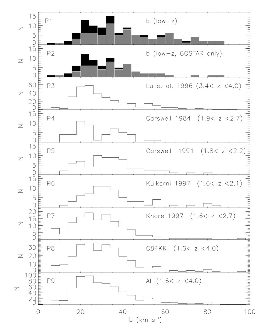
Figure 1: Top panel (P1) shows the low-$z$ distribution of line widths, $b$. Two features in the 3C 273 spectrum have been adjusted in accordance with Weymann et al. (1995). P2 shows only $b$-values obtained with HST+COSTAR. In P1 and P2, grey and black boxes indicate our $SL\geq 4\sigma$ and $3\sigma\leq SL<4\sigma$ samples, respectively. P3-P7 show higher-$z$  distributions from various sources (Table 3). Panel P8,“C84KK”, combines all the higher-$z$  distributions with resolutions comparable to ours ($\sim$19 km s^-1). P9, “All”, combines panels P3-P7.

3 Observed Rest-Frame Equivalent Width Distribution

In Figure 2 we display the rest-frame equivalent width ($\mathcal{W}$) distribution for all of our detected Ly$\alpha$ features. The solid grey boxes in Figure 2 represent our definite ($SL\geq 4\sigma$) sample, while the black boxes represent our possible ($3\sigma\leq SL<4\sigma$) sample. As expected, we detect an increasing number of absorbers at decreasing $\mathcal{W}$, down to our detection limit. As discussed in the previous section, our spectra are of varying sensitivity and wavelength coverage. This observed $\mathcal{W}$ distribution is not the true $\mathcal{W}$ distribution, because we have not yet accounted for incompleteness. To determine the true $\mathcal{W}$ distribution, we must normalize the $\mathcal{W}$ density by the available pathlength $\Delta$$z$($\mathcal{W}$).

The pathlength, $\Delta$$z$, is actually a function of $\mathcal{W}$ and $z$, since our spectra have varying 4$\sigma$ detection limits across the waveband and each spectrum covers a different waveband ($z$ range). Without this important sensitivity correction, $\Delta$$z$($\mathcal{W}$,$z$), any interpretation of the $\mathcal{W}$ distribution is premature. Previous studies, such as the HST/FOS Key project (Bahcall et al., 1993), avoided this problem by considering the $\mathcal{W}$ distribution only above a universal minimum $\mathcal{W}$ detectable in all portions of all spectra in the sample. This forces $\Delta$$z$($\mathcal{W}$,$z$) to be a constant pathlength, so that the $\mathcal{W}$ distribution is a true representation of the detected absorbers. However, this procedure eliminates information about the lowest, most numerous, $\mathcal{W}$ absorbers. Because our GHRS program probes the lowest equivalent widths of any low-$z$ Ly$\alpha$ program to date, it is important to use all available data for the weakest absorbers. In this section, we will explore the $\mathcal{W}$ distribution without regard to $z$ and neglect any evolution of $\mathcal{W}$ with $z$ (we find no evolution in numbers of Ly$\alpha$ absorbers with redshift over our small $\Delta$$z$ range). We will examine the $z$ distribution ($0.002<z<0.069$) and the $\mathcal{W}$ evolution with $z$ in later sections.

In Paper I, we discussed the available pathlength for each sightline in detail. In Figure 3, we display the available pathlength ($\Delta$$z$) in terms of $\mathcal{W}$ for each spectrum. The solid line in each panel indicates the full observational pathlength, uncorrected for the regions of spectra not available for Ly$\alpha$ detection due to Galactic, HVC, intrinsic, and non-Ly$\alpha$ intervening absorption lines as well as our “proximity effect” limit. This “proximity limit” ($cz_{AGN}-cz_{abs}>1,200$ km s^-1 ) eliminates potential absorption systems “intrinsic” to the AGN (see Paper I for a detailed description and justification). The dot-dashed line indicates the “effective” or available pathlength after we remove the spectral regions unavailable for Ly$\alpha$ detection. In Figure 3, $c\Delta$$z$($\mathcal{W}$) is given in units of Megameters per second (Mm s^-1  or 10³ km s^-1). Note that three targets (I ZW 1 (catalog ), Q1230+0115 (catalog ), and Markarian 501 (catalog )) have significantly poorer sensitivity than the rest of our sample and should be re-observed with HST, using the Space Telescope Imaging Spectrograph (STIS) or the Cosmic Origins Spectrograph (COS).

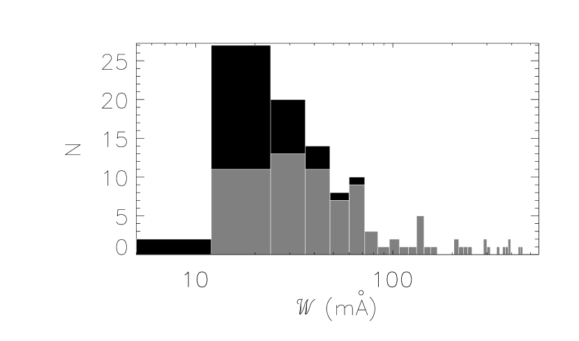
Figure 2: Observed distribution in rest-frame equivalent width ($\mathcal{W}$) of our detected Ly$\alpha$ absorbers. The solid grey boxes represent definite ($SL\geq 4\sigma$) detections, while the black boxes indicate possible ($3\sigma\leq SL<4\sigma$) absorbers. The $\mathcal{W}$ bins are 12 mÅ in width. This distribution has not been corrected for the non-uniform wavelength and sensitivity coverage of our observations. No intrinsic Ly$\alpha$ absorptions are included in this distribution.

In Figure 4, we display the cumulative distribution of $\Delta$$z$($\mathcal{W}$) for all spectra, for $SL\geq 4\sigma$ detections. In this cumulative plot, the solid line indicates the uncorrected pathlength. Also indicated is the pathlength available for Ly$\alpha$ detection after correcting for the spectral obscuration due to Galactic and HVC features, intrinsic and non-Ly$\alpha$ intervening absorbers (Intrinsic+Non-Ly$\alpha$), and our “proximity limit”. Indicated by the lowest (dotted) line is the cumulative available pathlength, for $SL\geq 4\sigma$ detections, after the indicated corrections have been made. The left axis of Figure 4 indicates the available pathlength ($c\Delta$$z$) in units of  Mm s^-1, while the right axis indicates $\Delta$$z$. Our maximum available pathlength ($c\Delta$$z$) is 116 Mm s^-1 (or $\Delta$$z$=0.387) for all features with $\mathcal{W}\geq 150$ mÅ. Also indicated in Figure 4 is our $N_{\rm HI}$ pathlength availability for a constant $b$=25 km s^-1. This pathlength compares to $\Delta z\approx 8$ at $z<0.3$ for the Key Project for strong absorbers ($\mathcal{W}>240$ mÅ).

Figure 3: Each panel shows the available pathlength, $c\Delta$$z$($\mathcal{W}$) in Mm s^-1, for a sightline as a function of 4$\sigma$ rest-frame equivalent width ($\mathcal{W}$). The solid line is the full $c\Delta$$z$, uncorrected for known Galactic, HVCs, intrinsic, or intervening features. Regions of FWHM$\times$2 of each $>$3$\sigma$ non-Ly$\alpha$ absorber are removed from the available $c\Delta$$z$ for detecting Ly$\alpha$ absorbers. The dashed line is the corrected $c\Delta$$z$, including the removal of 10 pixels ($\sim$0.2 Å) at each spectral edge and the application of our c$z_{\rm em}$– 1,200 km s^-1 “proximity limit”.

Figure 4: Cumulative available pathlength ($\Delta$$z$) as a function of $\mathcal{W}$, for $SL\geq 4\sigma$ detections. The left axis gives non-relativistic $c\Delta$$z$($\mathcal{W}$) in units of  Mm s^-1, while the right axis gives $\Delta$$z$. The solid (upper) line indicates the observed, uncorrected, $\Delta$$z$($\mathcal{W}$). Dashed, dot-dashed, and dot-dot-dashed lines indicate $c\Delta$$z$($\mathcal{W}$) after correcting for spectral obscuration due to non-Ly$\alpha$ and intrinsic absorption systems (Intrinsic+Non-Ly$\alpha$), Galactic and HVC absorption systems (Galactic+HVC), and our c$z_{\rm em}$– 1,200 km s^-1 “proximity” limit, respectively and individually. The dotted line indicates the fully corrected “effective” $\Delta$$z$($\mathcal{W}$), after the indicated spectral regions unavailable for intervening Ly$\alpha$ detection have been removed. Top axis indicates the $\log{\left[N_{\rm HI}\right]}$ corresponding to $\mathcal{W}$ for $b=25$ km s^-1; for example, $\log{\left[N_{\rm HI}\right]}=12.26$ for $\mathcal{W}=10$ mÅ (left-hand border of bottom axis).

3.1 The Low-$z$ Equivalent Width Distribution

In Figure 5, we apply the effective pathlength correction of Figure 4 to the $\mathcal{N}$($\mathcal{W}$) distribution of Figure 2. This procedure gives the true detected $\mathcal{W}$ number density,

$$n(\mathcal{W}_{i})=\mathcal{N}(\mathcal{W}_{i})/\Delta z(\mathcal{W}_{i})\Delta\mathcal{W}\approx{\partial^{2}\mathcal{N}/\partial z~{}\partial\mathcal{W}}~{}|_{\mathcal{W}_{i}},$$ (1)

corrected for the pathlength, $\Delta$$z$($\mathcal{W}_{i}$), available to detect features at each $\mathcal{W}_{i}$, without regard to $z$. The approximation that $n(\mathcal{W})$ is equal to d$\mathcal{N}$/d$\mathcal{W}$ is limited by our sample size ($\mathcal{N}$) and by our bin size ($\Delta$$\mathcal{W}$= 12 mÅ). However, this approximation is more than sufficient for our purposes.

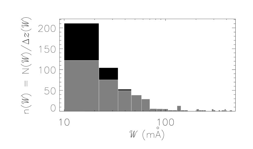
Figure 5: Rest-frame equivalent width ($\mathcal{W}$) number distribution, $n(\mathcal{W})$, corrected for available pathlength ($\Delta$$z$). The corrected number density, $n(\mathcal{W})$=$\mathcal{N}$($\mathcal{W}$)/$\Delta$$z$($\mathcal{W}$), is the observed $\mathcal{W}$ distribution corrected for the non-uniform sensitivity function of our observations. The solid grey boxes represent definite ($SL\geq 4\sigma$) detections, while the black boxes indicate possible ($3\sigma\leq SL<4\sigma$) absorbers. The $\mathcal{W}$ bins are 12 mÅ in width.

It has been shown (Sargent et al., 1980; Young, Sargent, & Boksenberg, 1982; Murdoch et al., 1986; Weymann et al., 1998) that ${\partial^{2}\mathcal{N}/\partial z~{}\partial\mathcal{W}}$, the pathlength-corrected number density of lines with respect to $\mathcal{W}$, is well modeled by $n(\mathcal{W})=\left(C_{\mathcal{W}}/\mathcal{W}_{\star}\ \right)\exp\left(-\mathcal{W}/\mathcal{W}_{\star}\ \right)$, where $\mathcal{W}_{\star}$  is the characteristic equivalent width and $C_{\mathcal{W}}$ is the characteristic line density per unit redshift. In Figure 6, $n(\mathcal{W})$ is plotted versus $\mathcal{W}$ in natural logarithmic form, for both our definite ($SL\geq 4\sigma$) and our expanded ( Ly$\alpha$ samples. Our $\mathcal{W}$ bins are 12 mÅ in width, and our upper $\mathcal{W}$ cutoff is 133 mÅ. Also indicated by dashed lines in Figure 6 is our least-squares fit to $\ln\left[n(\mathcal{W})\right]=\ln\left[C_{\mathcal{W}}/\mathcal{W}_{\star}\ \right]-\mathcal{W}/\mathcal{W}_{\star}\$ for $10~{}{\rm m}\mbox{\AA}<\mathcal{W}<133~{}{\rm m}\mbox{\AA}$. For our definite sample, $\mathcal{W}_{\star}$ $=27\pm 5$ mÅ and $C_{\mathcal{W}}$$=520\pm 179$ mÅ. For our expanded sample over the same $\mathcal{W}$ interval, $\mathcal{W}_{\star}$ $=23\pm 3$ mÅ and $C_{\mathcal{W}}$$=733\pm 205$ mÅ.

For comparison, at higher redshift, Sargent et al. (1980) obtained $\mathcal{W}_{\star}=362\pm 21$ mÅ, $C_{\mathcal{W}}=154\pm 11$ mÅ, while Young, Sargent, & Boksenberg (1982) obtained $\mathcal{W}_{\star}=232\pm 34$ mÅ, $C_{\mathcal{W}}=135\pm 20$ mÅ in the redshift range $1.7<z\ <3.3$ for Ly$\alpha$ absorbers with $\mathcal{W}\geq 160$ mÅ. At first comparison, our results seem inconsistent with these results. However, as has been noted (Murdoch et al., 1986; Carswell et al., 1984; Atwood, Baldwin, & Carswell, 1985), the parameters $\mathcal{W}_{\star}$ and $C_{\mathcal{W}}$ are highly dependent on the spectral resolution of the observations, mostly because at higher resolution blended lines break up into components. One sample that approximates our resolution and sensitivity is that of Carswell et al. (1984). Based upon 20 km s^-1 resolution optical data, Carswell et al. (1984) obtained $\mathcal{W}_{\star}=70\pm 20$ mÅ for their unblended, $\mathcal{W}>133~{}{\rm m}\mbox{\AA}$, Ly$\alpha$ sample.

Figure 6: The differential distribution, $n(\mathcal{W})$= ${\partial^{2}\mathcal{N}/\partial z~{}\partial\mathcal{W}}$, plotted in natural logarithm form. The $n(\mathcal{W})$ error bars are based upon $\sqrt{N}$ statistics. The left panel indicates the distribution for our definite ($SL\geq 4\sigma$) Ly$\alpha$ absorbers only. The right panel includes the distribution for our expanded ( Ly$\alpha$ sample. The $\mathcal{W}$ bins are 12 mÅ and only Ly$\alpha$ absorbers with $\mathcal{W}<133~{}{\rm m}\mbox{\AA}$ are included.

As indicated in Murdoch et al. (1986, their Figure 3), there is evidence for a break in the slope of $n(\mathcal{W})$ below 200 mÅ. As shown in Figure 7, we confirm this break, even though our statistics in this region ($\mathcal{W}$ $>$200 mÅ) are poor. For $b$=25 km s^-1, this corresponds to a break at $\log{\left[N_{\rm HI}\right]}$$\sim$14.0. The reality of this break will be discussed further in § 4, which focuses on the $N_{\rm HI}$ distribution of the low-$z$ Ly$\alpha$ forest.

At first consideration, the presence of this break is intriguing. However, one must understand the nature of this discontinuity in relation to the Ly$\alpha$ curve of growth to gauge its significance. As pointed out by Jenkins & Ostriker (1991) and Press & Rybicki (1993), this upturn in the number of low $\mathcal{W}$ clouds can be explained by the transition from saturated to unsaturated lines. The form of $n(\mathcal{W})$=$\left(C_{\mathcal{W}}/\mathcal{W}_{\star}\right)\exp{\left(-\mathcal{W}/\mathcal{W}_{\star}\right)}$ is designed to model absorbers in the logarithmic or flat part of the curve of growth. As discussed in § 4, it has been shown that at higher column densities, Ly$\alpha$ absorbers appear to follow the distribution $n(N_{\rm HI})=\partial^{2}\mathcal{N}/\partial z~{}\partial N_{\rm HI}=C_{\rm HI}N_{\rm HI}^{-\beta}$. On the linear portion of the curve of growth, where $\mathcal{W}=AN_{\rm HI}$,

$${n(\mathcal{W})={\partial^{2}\mathcal{N}\over\partial z~{}\partial\mathcal{W}}={\partial^{2}\mathcal{N}\over\partial z~{}\partial N_{\rm HI}\ }{{\rm d}N_{\rm HI}\ \over{\rm d}\mathcal{W}}={C_{\rm HI}N_{\rm HI}^{-\beta}\over A}~{}~{}{\rm~{},~{}or}}$$ (2)

$${n(\mathcal{W})={C_{\rm HI}\left(\mathcal{W}/A\right)^{-\beta}\over A}=A^{\beta-1}~{}C_{\rm HI}~{}\mathcal{W}^{-\beta}.}$$ (3)

As derived in equation (23) for Ly$\alpha$, A = $54.43\times 10^{-13}$ mÅ for $N_{\rm HI}$ in $10^{13}$  cm^-2 and $\mathcal{W}$ in mÅ.

In Figure 7 we add our absorbers with $\mathcal{W}>133~{}{\rm m}\mbox{\AA}$ to the $SL\geq 4\sigma$ $\ln{[n(\mathcal{W})]}$ distribution of Figure 6. We increase the upper $\mathcal{W}$ bin size from 12 mÅ to 42 mÅ to compensate for our poor statistics, so that there is at least one absorber in each bin. Above $\mathcal{W}$ = 133 mÅ, we obtain $\mathcal{W}_{\star}=259\pm 180$ mÅ and $C_{\mathcal{W}}=138\pm 129$ mÅ. Below 133 mÅ, we fit by equation (3), using the least-squares method, and find $\beta=1.89\pm 0.39$ for our $SL\geq 4\sigma$ sample ($\beta=2.20\pm 0.37$ for our sample). The value of $C_{\rm HI}$ is not well constrained due to the exponential nature of this fitting method, but the best fit gives $C_{\rm HI}~{}\sim 4\times 10^{14}$.

Figure 7: The differential distribution, $n(\mathcal{W})$= ${\partial^{2}\mathcal{N}/\partial z~{}\partial\mathcal{W}}$, of Ly$\alpha$ absorbers with respect to $\mathcal{W}$ is plotted in natural logarithm form, for our $SL\geq 4\sigma$  Ly$\alpha$ sample. The $n(\mathcal{W})$ error bars are based upon $\sqrt{N}$ statistics. The $\mathcal{W}$ range has been expanded to include all detected Ly$\alpha$ absorbers. Below $\mathcal{W}$ = 133 mÅ, the $\mathcal{W}$ bins are 12 mÅ in width; above 133 mÅ the bins are 42 mÅ wide. Horizontal (1$\sigma$) error bars are set to 1/3 of the $\mathcal{W}$ bin widths.

3.2 Integrated d$\mathcal{N}$/d$z$ Results

By integrating ${\partial^{2}\mathcal{N}/\partial z~{}\partial\mathcal{W}}$ from $\mathcal{W}$ to $\infty$, we can determine the number density of lines per unit redshift, d$\mathcal{N}$/d$z$ , stronger than $\mathcal{W}$. As stated previously, we have assumed no evolution with $z$ over our small range for Ly$\alpha$ detection ($0.002<z<0.069$). Because of our very low-$z$ range, these values for d$\mathcal{N}$/d$z$ are a good approximation of (d$\mathcal{N}$/d$z$)_z=0. Figure 8 shows d$\mathcal{N}$/d$z$ , defined as

$${\rm d}\mathcal{N}/{\rm d}z\ (\mathcal{W}~{}>\mathcal{W}_{i})=\int_{\mathcal{W}_{i}}^{\infty}{\partial^{2}\mathcal{N}\over\partial z~{}\partial\mathcal{W}}~{}{\rm d}\mathcal{W}.$$ (4)

The vertical axis of Figure 8 gives (d$\mathcal{N}$/d$z$)_z=0  in terms of both $\mathcal{W}$ (lower axis) and $\log{\left[N_{\rm HI}\right]}$ (upper axis, assuming that all absorbers are single components with $b$-values of 25 km s^-1).

For comparison, Table 4 gives (d$\mathcal{N}$/d$z$)_z=0  from other HST absorption-line studies, along with our low-$z$ results for their observational $\mathcal{W}$ limits ($\mathcal{W}$_min). The detection limits of the various HST spectrographs and gratings are indicated by the dashed vertical lines in Figure 8. The unlabeled vertical line on the far left of Figure 8 in the GHRS/G140L+G160M merged sample of Tripp, Lu, & Savage (1998). In all cases, our values for (d$\mathcal{N}$/d$z$)_z=0 at various limiting $\mathcal{W}$ are slightly greater than those derived from higher limiting $\mathcal{W}$ studies at low-$z$ , but are still within the 1$\sigma$ error ranges. The value of d$\mathcal{N}$/d$z$ at the present epoch ($z$=0) is an important constraint for hydrodynamical cosmological models attempting to reproduce the observed baryon distribution of the Universe (Davé et al., 1999). The (d$\mathcal{N}$/d$z$)_z=0 values of our GHRS survey have the lowest measured $\mathcal{W}$ values to date. In § 5.1, these values will be used to place important constraints upon the $z$-evolution of d$\mathcal{N}$/d$z$.

Figure 8: Integrated d$\mathcal{N}$/d$z$ above $\mathcal{W}$: ${\rm d}\mathcal{N}/{\rm d}z\ (\mathcal{W}~{}>\mathcal{W}_{i})=\int_{\mathcal{W}_{i}}^{\infty}({\partial^{2}\mathcal{N}/\partial z~{}\partial\mathcal{W}}){\rm d}\mathcal{W}$, for our $SL\geq 4\sigma$ sample. For clarity, we plot every third error bar. The $\mathcal{W}$ bins are 12 mÅ, connected by the solid line. Also shown by dotted vertical lines are the minimum $\mathcal{W}$ limits for the various HST Ly$\alpha$ surveys presented in Table 4. The unlabeled vertical dashed line on the far left corresponds to the Tripp, Lu, & Savage (1998) G140L+G160M combined sample (see Table 4). The horizontal axes begin at $\mathcal{W}$ = 10 mÅ or $\log{\left[N_{\rm HI}\right]}$= 12.26.

Table 4: (d$\mathcal{N}$/d$z$)_z=0 Determinations From Other Ly$\alpha$ Studies

Reference	Instrument/	$z$ range	$\mathcal{W}$min	(d$\mathcal{N}$/d$z$)z=0	Our (d$\mathcal{N}$/d$z$)z=0
	Configuration		(mÅ)		at $\mathcal{W}$min
Bahcall et al. 1993a	FOS	0$<z<$1.3	320	17.7$\pm$4.3	18.2$\pm$6.9
Bahcall et al. 1996	FOS	0$<z<$1.3	240	24.3$\pm$6.6	28.5$\pm$8.6
Weymann et al. 1998	FOS	0$<z<$1.5	240	32.7$\pm$4.2	28.5$\pm$8.6
Impey et al. 1999	GHRS/G140L	0$<z<$0.22	240	38.3$\pm$5.3	28.5$\pm$8.6
Tripp et al. 1998	GHRS/G140L	0$<z<$0.28	75	71$\pm$12	80.0$\pm$14.6
Tripp et al. 1998	GHRS/G140L	0$<z<$0.28	50	102$\pm$16	134.2$\pm$20.1

3.3 Rest-Frame Equivalent Width versus $b$ Distribution

In Figure 9, we plot the observed $\mathcal{W}$ distribution versus the resolution-corrected $b$ values. In this figure, the 81 definite absorbers are plotted as small dots while the 30 possible ($3\sigma\leq SL<4\sigma$) Ly$\alpha$ detections are plotted as diamonds. In neither sample do we detect any correlation of $\mathcal{W}$ with respect to $b$ (in the definite sample the correlation coefficient is zero). Since very broad weak features are indistinguishable from small continuum fluctuations, we may not be sensitive to features in the lower right corners (large $b$-values and low $\mathcal{W}$) of Figure 9. A completely homogeneous distribution would be created in Figure 9 by adding $\sim$15 absorbers at $\mathcal{W}\leq 30$ mÅ and $b=60-100$ km s^-1. At the spectral resolution of these observations these absorbers have maximum deflections of $<15\%$ of the base continuum level and thus would be extremely difficult to distinguish from a slight undulation in the continuum. Therefore, given the absence of reliable $b$-values for each absorber and no obvious $b$-$\mathcal{W}$ correlation, we will assume a single $b$-value when calculating $N_{\rm HI}$. Figure 9 shows that there is no obvious bias in making this single $b$-value choice.

Figure 9: Distribution of rest-frame equivalent width ($\mathcal{W}$) versus $b$-value of our detected Ly$\alpha$ absorbers. The left panel displays the distribution of the definite ($SL\geq 4\sigma$) sample with error bars. The right panel shows the $SL\geq 4\sigma$ sample as dots, combined with the $3\sigma\leq SL<4\sigma$ sample displayed as diamonds, forming our expanded sample. The absence of absorbers in the lower right corners is related to an insensitivity to very broad weak features, which could be interpreted as continuum fluctuations.

4 Observed H I Column Densities

In Table 1, we estimated the neutral hydrogen column density ($N_{\rm HI}$) of each detected $SL\geq 4\sigma$ (definite) Ly$\alpha$ absorber from its equivalent width, assuming a single component with a $b$-value of 20, 25, 30 km s^-1, and the measured $b$ values. Table 2 presents $N_{\rm HI}$ results for our $3\sigma\leq SL<4\sigma$ (possible) Ly$\alpha$ sample. As described in Paper I and in § 2, the observed $b$-values have been corrected for the HST+GHRS/G160M instrumental profile and our pre-fit smoothing. Columns 4 and 5 of Tables 1 and 2 indicate the measured $b$-values ($b_{\rm obs}$) and the corrected $b$-values ($b$), respectively. Figure 10 compares the results on $\log{\left[N_{\rm HI}\right]}$ of our sample for these various $b$-values.

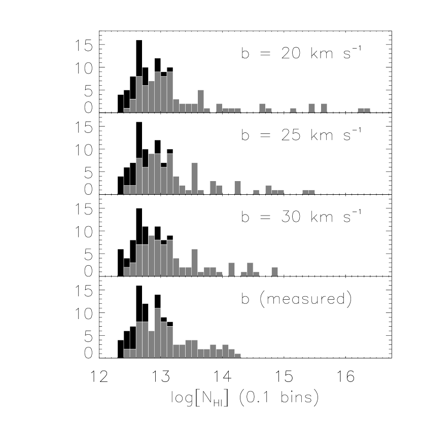
Figure 10: H I column densities, $N_{\rm HI}$ , of our observed low-$z$ Ly$\alpha$ absorbers for various $b$-values. The top three panels show the distribution based upon all features having a single $b$-value of 20, 25, or 30 km s^-1 as indicated. Bottom panel shows the distribution based upon $b$-values measured from Gaussian components and corrected by the HST+GHRS/G160M resolution element. The grey absorbers are our definite ($SL\geq 4\sigma$) sample, while the black absorbers are our possible ($3\sigma\leq SL<4\sigma$) sample.

Below $\log{\left[N_{\rm HI}\right]}$$\sim$13, all the $N_{\rm HI}$ distributions of Figure 10 are similar, because the Ly$\alpha$ absorbers are on the linear part of the curve of growth where $N_{\rm HI}$ does not depend on the $b$-value. Above $\log{\left[N_{\rm HI}\right]}$= 14, the Ly$\alpha$ absorbers are partially saturated for $b$=25$\pm$ 5 km s^-1. For Gaussian line profiles, the optical depth at the line center is given by:

$${\tau_{0}=\left(0.303\right)\left[N_{\rm HI}\ \over 10^{13}\ {\rm cm}^{-2}~{}\right]\left[25~{}{\rm km~{}s}^{-1}\over b\right]\ \ {\rm.}}$$ (5)

Figure 11: The low-$z$ Ly$\alpha$ number distribution per unit redshift and column density, $n(N_{\rm HI})$=$\partial^{2}\mathcal{N}/\partial z~{}\partial N_{\rm HI}$, for a constant $b$-value of 25 km s^-1and $\log{\left[N_{\rm HI}\right]}<14.0$. The $n(N_{\rm HI})$ error bars are based upon $\sqrt{N}$ statistics. The left panel indicates the distribution for our definite ($SL\geq 4\sigma$) Ly$\alpha$ absorbers only. The right panel includes the distribution for our expanded ( Ly$\alpha$ sample.

On the logarithmic or flat-part of the curve of growth, $N_{\rm HI}$ depends on the $b$-values. Above $\log{\left[N_{\rm HI}\right]}$$\sim$18.5, the Ly$\alpha$ absorbers develop damping wings, and $N_{\rm HI}$ is once again insensitive to the $b$-value. None of our detected Ly$\alpha$ absorbers has $\log{\left[N_{\rm HI}\right]}$$>$17. While we believe this to be a typical range of true values for our detections, clearly there is some uncertainty in the individual values of $N_{\rm HI}$ at $\log{\left[N_{\rm HI}\right]}\geq 13.5$.

The $N_{\rm HI}$ number density per unit redshift and column density is often modeled by a power-law distribution:

$${{\partial^{2}\mathcal{N}\over\partial z~{}\partial N_{\rm HI}\ }\sim{N\left(N_{\rm HI}\right)\over\Delta z\left(N_{\rm HI}\right)\Delta N_{\rm HI}}\equiv n(N_{\rm HI})=C_{\rm HI}~{}N_{\rm HI}^{-\beta}~{}~{}.}$$ (6)

In Figure 11, we display $\log\left[n(N_{\rm HI})\right]$ for both our definite ($SL\geq 4\sigma$) and expanded ( Ly$\alpha$ samples over the range $12.3\leq\log{\left[N_{\rm HI}\right]}\leq 14.0$. Also indicated in Figure 11 are the least-squares fits to $\log\left[n(N_{\rm HI})\right]=\log\left[C_{\rm HI}\right]-\beta$ $\log{\left[N_{\rm HI}\right]}$. Using a $b$-value of 25 km s^-1 for all features, we obtain $\beta=1.83\pm 0.15$ and $\log\left[C_{\rm HI}\right]=12.8\pm 1.9$ for our definite sample and $\beta=1.81\pm 0.12$ and $\log\left[C_{\rm HI}\right]=12.6\pm 1.6$ for our expanded sample over the range $12.3\leq\log{\left[N_{\rm HI}\right]}\leq 14.0$. There is no evidence for a turnover of $n(N_{\rm HI})$ below $N_{\rm HI}\ =10^{12.5}$ cm^-2 in either our definite or expanded Ly$\alpha$ samples. The determination of $\beta$ and $C_{\rm HI}$ is insensitive to $b$-value below $\log{\left[N_{\rm HI}\right]}\leq 14$, since all absorbers are then on or near the linear portion of the Ly$\alpha$ curve of growth, which is independent of $b$-value.

Above $\log{\left[N_{\rm HI}\right]}$$\sim$14, the Ly$\alpha$ absorbers become partially saturated, and the choice of $b$-value becomes important in determining $N_{\rm HI}$. As shown in Figure 12, we detect a break in the $N^{-\beta}_{\rm HI}$ power-law above $\log{\left[N_{\rm HI}\right]}$$\sim$14, which is possibly related to saturation or poor line statistics. However, Kulkarni et al. (1996) detect a similar break in the region of $N_{\rm HI}$ $\sim$10^14.5 cm^-2 for Ly$\alpha$ absorbers at $1.7<z<2.1$. Figure 12 compares the power-laws for the two column density regimes, $12.3\leq\log{\left[N_{\rm HI}\right]}\leq 14.0$ and $14.0\leq\log{\left[N_{\rm HI}\right]}\leq 16.0$, for both our definite ($SL\geq 4\sigma$) and expanded samples (, again for a constant $b$=25 km s^-1. Since none of the strong absorbers ($\log{\left[N_{\rm HI}\right]}$$>$ 14.0) are tentative detections ($3\sigma\leq SL<4\sigma$), the results for the definite and expanded samples are identical with $\beta=1.04\pm 0.39$ and $\log\left[C_{\rm HI}\right]=1.5\pm 5.7$. The large uncertainties are a reflection of the poor number statistics.

Table 5: Differential, $n(N_{\rm HI})$, and integrated, $I(N_{\rm HI})$, determinations of $\beta$ and log[$C_{\rm HI}$] for the low-$z$ Ly$\alpha$ absorbers.

12.3 $\leq$ log[$N_{\rm HI}$ ] $\leq$ 14.0
		Differential		Integrated
Sample	$b$-value	$\beta$	log[$C_{\rm HI}$ ]	$\beta$	log[$C_{\rm HI}$ ]	$N$
Definite	20	1.83 $\pm$0.16	12.8 $\pm$ 2.1	1.70 $\pm$0.05	11.0 $\pm$ 0.7	68
Definite	25	1.83 $\pm$0.15	12.8 $\pm$ 1.9	1.72 $\pm$0.06	11.3 $\pm$ 0.7	71
Definite	30	1.80 $\pm$0.15	12.5 $\pm$ 2.0	1.74 $\pm$0.06	11.5 $\pm$ 0.7	71
Definite	$b$	1.84 $\pm$0.14	13.0 $\pm$ 1.9	1.77 $\pm$0.06	11.9 $\pm$ 0.8	75
Expanded	20	1.81 $\pm$0.13	12.6 $\pm$ 1.7	1.78 $\pm$0.05	12.1 $\pm$ 0.6	98
Expanded	25	1.81 $\pm$0.12	12.6 $\pm$ 1.6	1.81 $\pm$0.05	12.4 $\pm$ 0.7	101
Expanded	30	1.80 $\pm$0.12	12.5 $\pm$ 1.6	1.83 $\pm$0.05	12.7 $\pm$ 0.7	101
Expanded	$b$	1.83 $\pm$0.11	12.8 $\pm$ 1.5	1.86 $\pm$0.06	13.0 $\pm$ 0.7	105
14.0 $\leq$ log[$N_{\rm HI}$ ] $\leq$ 16.0
		Differential		Integrated
Sample	$b$-value	$\beta$	log[$C_{\rm HI}$ ]	$\beta$	log[$C_{\rm HI}$ ]	$N$
Definite/Expanded	20	1.07 $\pm$0.18	2.0 $\pm$ 2.7	1.34 $\pm$0.13	6.2 $\pm$ 1.9	13
Definite/Expanded	25	1.04 $\pm$0.39	1.5 $\pm$ 5.7	1.43 $\pm$0.35	7.4 $\pm$ 5.2	10
Definite/Expanded	30	1.40 $\pm$0.64	6.7 $\pm$ 9.5	1.81 $\pm$0.73	12.6 $\pm$10.7	10
12.3 $\leq$ log[$N_{\rm HI}$ ] $\leq$ 16.0
		Differential		Integrated
Sample	$b$-value	$\beta$	log[$C_{\rm HI}$ ]	$\beta$	log[$C_{\rm HI}$ ]	$N$
Definite	20	1.44 $\pm$0.07	7.6 $\pm$ 1.0	1.53 $\pm$0.04	8.9 $\pm$ 0.5	81
Definite	25	1.58 $\pm$0.10	9.6 $\pm$ 1.4	1.66 $\pm$0.06	10.5 $\pm$ 0.8	81
Definite	30	1.64 $\pm$0.12	10.3 $\pm$ 1.7	1.71 $\pm$0.08	11.3 $\pm$ 1.0	81
Definite	$b$	1.60 $\pm$0.17	9.8 $\pm$ 2.3	1.77 $\pm$0.11	11.9 $\pm$ 1.4	81
Expanded	20	1.50 $\pm$0.07	8.5 $\pm$ 0.9	1.57 $\pm$0.04	9.5 $\pm$ 0.5	111
Expanded	25	1.65 $\pm$0.10	10.4 $\pm$ 1.4	1.71 $\pm$0.06	11.3 $\pm$ 0.8	111
Expanded	30	1.71 $\pm$0.12	11.2 $\pm$ 1.6	1.78 $\pm$0.08	12.1 $\pm$ 1.0	111
Expanded	$b$	1.70 $\pm$0.16	11.1 $\pm$ 2.2	1.85 $\pm$0.11	13.0 $\pm$ 1.4	111

Figure 12: The differential low-$z$ Ly$\alpha$ number distribution per unit redshift and column density, $n(N_{\rm HI})$=$\partial^{2}\mathcal{N}/\partial z~{}\partial N_{\rm HI}\$, over the range $12.3\leq\log{\left[N_{\rm HI}\right]}\leq 16.0$  for a constant $b$-value of 25 km s^-1. The $n(N_{\rm HI})$ error bars are based upon $\sqrt{N}$ statistics. The upper panel indicates the distribution for definite ($SL\geq 4\sigma$) Ly$\alpha$ absorbers only. The lower panel includes the distribution for expanded ( Ly$\alpha$ sample. Indicated on each panel are the best-fit power-laws for each $\log{\left[N_{\rm HI}\right]}$ regime, $12.3\leq\log{\left[N_{\rm HI}\right]}\leq 14.0$ and $14.0\leq\log{\left[N_{\rm HI}\right]}\leq 16.0$. In the lower $N_{\rm HI}$ regime, the $\log{\left[N_{\rm HI}\right]}$ bins are 0.12, while in the upper regime the bins are 0.40.

To obtain better determinations of $\beta$ and $C_{\rm HI}$ , we evaluate the integrated $n(N_{\rm HI})$,

$$I(N_{\rm HI})=\int_{N_{\rm HI}\ }^{\infty}C_{\rm HI}~{}N_{\rm HI}^{-\beta}{\rm d}N_{\rm HI}\ ={C_{\rm HI}~{}\over 1-\beta}~{}N_{\rm HI}^{1-\beta}.$$ (7)

Table 5 compares our results for both the differential, $n(N_{\rm HI})$, and integrated, $I(N_{\rm HI})$, determinations of $\beta$ and $C_{\rm HI}$ for $b$-values of 20, 25, 30 km s^-1 and $b$. This table is divided into three $\log{\left[N_{\rm HI}\right]}$ ranges over which least-squares determinations of $\beta$ and $C_{\rm HI}$ are performed: $12.3\leq\log{\left[N_{\rm HI}\right]}\leq 14.0$, $14.0\leq\log{\left[N_{\rm HI}\right]}\leq 16.0$, and the full range $12.3\leq\log{\left[N_{\rm HI}\right]}\leq 16.0$. Results are given for both our definite and expanded Ly$\alpha$ samples. By column Table 5 includes: (1) sub-sample name; (2) $b$-value assumed in km s^-1; (3-6) best-fit values for $\beta$ and $\log\left[C_{\rm HI}\right]$ in cm^-2 for both differential and integral counts; and (7) the number of absorption lines in each subsample. Note that the results over the range $14.0\leq\log{\left[N_{\rm HI}\right]}\leq 16.0$ are the same for the definite and expanded samples since these data sets are identical over this $\log{\left[N_{\rm HI}\right]}$ range. When using our measured $b$-values, all features in this column density range occur in the same $\log{\left[N_{\rm HI}\right]}$ bin. Hence we cannot report values for this column density range for these $b$-values. Using the integrated $I(N_{\rm HI})$ rather than the differential distribution $n(N_{\rm HI})$ to determine $\beta$ and $C_{\rm HI}$ is more robust since it uses the cumulative $N_{\rm HI}$ distribution, instead of the individual $N_{\rm HI}$ bin values in the parameter determination. Using the integrated distributions for $b$=25 km s^-1, we obtain $\beta=1.72\pm 0.06$ and $\log\left[C_{\rm HI}\right]=11.3\pm 0.7$ for our definite sample and $\beta=1.81\pm 0.05$ and $\log\left[C_{\rm HI}\right]=12.4\pm 0.7$ for our expanded sample over the range $12.3\leq\log{\left[N_{\rm HI}\right]}\leq 14.0$.

As indicated in Table 5, the values for $\beta$ that we obtain over the column density range $12.3\leq\log{\left[N_{\rm HI}\right]}\leq 14.0$ are consistently $>$1.7. This value is in agreement with our results of § 3, where we fitted $n(\mathcal{W})$$\propto$ $\mathcal{W}$^-β and obtained $\beta=1.89\pm 0.39$. We derive our best values from the integrated $SL\geq 4\sigma$ sample, using a constant value $b$=25 km s^-1:

$${\beta=1.72\pm 0.06~{},~{}\log\left[C_{\rm HI}\right]=11.3\pm 0.7~{}{\rm for}~{}12.5\leq\log{\left[N_{\rm HI}\right]}\leq 14.0,}$$ (8)

$${\beta=1.43\pm 0.35~{},~{}\log\left[C_{\rm HI}\right]=7.4\pm 5.2~{}{\rm for}~{}14.0\leq\log{\left[N_{\rm HI}\right]}\leq 16.0\ {\rm,}}$$ (9)

$${\beta=1.66\pm 0.06~{},~{}\log\left[C_{\rm HI}\right]=10.5\pm 0.8~{}{\rm for}~{}12.5\leq\log{\left[N_{\rm HI}\right]}\leq 16.0.}$$ (10)

These results are in contrast with the recent higher-$z$ results of Kim et al. (1997), Lu et al. (1996), and Hu et al. (1995), who find that $\beta$$\sim$1.4 adequately describes $n(N_{\rm HI})$ for 12.3$<$$\log{\left[N_{\rm HI}\right]}$$<$14.3 over the redshift range 2.17$<$$z$$<$4.00. In conjunction with other studies between $z$=4 and $z$=2, these authors claim that the $n(N_{\rm HI})$ break appears to strengthen and move to lower column densities with decreasing redshift. Furthermore, Kim et al. (1997) report a break in $n(N_{\rm HI})$ above $\log{\left[N_{\rm HI}\right]}\geq 14.3$ that steepens ($\beta=1.7-1.8$) and moves to lower column density with decreasing redshift (2.17$<$$z$$<$4.0). In contrast, at low-$z$ we see a flattening in $n(N_{\rm HI})$ above $\log{\left[N_{\rm HI}\right]}$=14.0. It is possible that the apparent flattening in our data is an artifact of our selection of a constant $b$-value for all Ly$\alpha$ absorbers. If the stronger Ly$\alpha$ absorbers had larger $b$-values, then the inferred column densities of these features could be much smaller. This would leave us with fewer features above $\log{\left[N_{\rm HI}\right]}$$>$14, and therefore no evidence for a break in $n(N_{\rm HI})$  at $\log{\left[N_{\rm HI}\right]}=14.0$. In § 5.3, we will examine the possibility that the break in $n(N_{\rm HI})$  is a consequence of the $z$ evolution of $\partial^{2}\mathcal{N}/\partial z~{}\partial N_{\rm HI}\$.

5 Observed Redshift Distribution

In this section, we examine the redshift distribution of the low-$z$ Ly$\alpha$ forest. In particular, we want to examine the evidence for structure at specific redshifts, or for any evolution of d$\mathcal{N}$/d$z$ with $z$. We begin with Figure 13, a presentation of the observed number distribution per redshift bin without any sensitivity correction, $\mathcal{N}$($z$), for both our definite and expanded Ly$\alpha$ samples. The left axis corresponds to the displayed histograms of $\mathcal{N}$($z$). Our redshift range, $0.002<z<0.069$, is divided into 12 redshift bins, $\delta$$z$= 0.0056. Individual $SL\geq 4\sigma$ Ly$\alpha$ absorbers are plotted as pluses, whose $\mathcal{W}$(mÅ) is shown on the right vertical axis. Individual $3\sigma\leq SL<4\sigma$  Ly$\alpha$ absorbers are plotted as ‘x’s. Like the $\mathcal{N}$($\mathcal{W}$) distribution, the $\mathcal{N}$($z$) distribution is not the true redshift distribution, because we have not corrected for the varying wavelength and sensitivity coverage of our observations.

We show the correction for our varying wavelength and sensitivity coverage, $\Delta$$z$($z$), in Figure 14. In this figure, the panels show various stages of correction for the cumulative distribution of $\Delta$$z$($z$) for $SL\geq 4\sigma$ detections in all sightlines. The upper panel of Figure 14 presents the full pathlength availability of our sample. The left axis gives $c\Delta$$z$($z$) in  Mm s^-1, while the right axis is in redshift units. Subsequent panels present the available pathlength after removing portions of our wavelength coverage due to obscuration by extragalactic non-Ly$\alpha$ features and intrinsic features (Intrinsic+Non-Ly$\alpha$), by Galactic+HVC features, and by our c$z_{\rm em}$– 1,200 km s^-1 proximity limit. The bottom panel presents the pathlength available after removing all spectral regions not suitable for detecting intervening Ly$\alpha$ absorbers. The available pathlength in Figure 14 approximately represents $\Delta$$z$($z$) for features with $\mathcal{W}$$>$150 mÅ. As presented in Figure 4, our pathlength is approximately constant at $c\Delta$$z$($\mathcal{W}$)=0.387 for $\mathcal{W}$$>$150 mÅ.

Figure 13: Histogram of $\mathcal{N}$($z$) and distribution of rest-frame equivalent width ($\mathcal{W}$) versus redshift. The histograms correspond to the left axis and indicate $\mathcal{N}$($z$), the number of absorbers per redshift bin ($\delta$$z$). The solid histogram indicates the distribution of the definite ($SL\geq 4\sigma$) Ly$\alpha$ sample, while the dotted distribution is for the expanded ( Ly$\alpha$ sample. The pluses (‘+’) and x’s correspond to the right axis and indicate $\mathcal{W}$ of the individual Ly$\alpha$ absorbers in the definite and possible ($3\sigma\leq SL<4\sigma$) samples, respectively.

Figure 14: Cumulative available pathlength ($\Delta$$z$) for all sightlines as a function of $z$, for features with $\mathcal{W}>150$ mÅ. Left axis gives $c\Delta$$z$($z$) in units of  Mm s^-1, while the right axis gives $\Delta$$z$($z$) in terms of $z$. The upper panel presents the full, uncorrected $\Delta$$z$($z$). Subsequent panels present $\Delta$$z$($z$) after removing portions of our wavelength coverage due to obscuration by extragalactic non-Ly$\alpha$ features, Galactic + HVC features, and the (c$z_{\rm em}$– 1,200 km s^-1) proximity limit. The bottom panel presents our $c\Delta$$z$($z$) for detecting intervening Ly$\alpha$ absorbers after applying these corrections.

To properly characterize the low-$z$ Ly$\alpha$ absorber distribution in redshift, one must accurately account for varying available pathlength as a function of both $N_{\rm HI}$ and $z$ of the observations. Figure 15 displays the combined two-dimensional sensitivity function, $c\Delta$$z$($N_{\rm HI}$,$z$), for GHRS/160M observations as a function of $z$ and $N_{\rm HI}$, after accounting for the aforementioned corrections and obscurations.

Figure 15: Bivariate pathlength sensitivity correction, $c\Delta$$z$($N_{\rm HI}$,$z$). The sensitivity function corrects $\partial^{2}\mathcal{N}/\partial z~{}\partial N_{\rm HI}\$by accounting for varying regions of $N_{\rm HI}$ sensitivity and $z$ coverage. The vertical axis indicates the available pathlength (in  Mm s^-1) for a given column density, $N_{\rm HI}$, and redshift (wavelength). When viewed from the column density axis, this figure reduces to the dotted line in Figure 4, and when viewed from the redshift axis, the bottom plot of Figure 14 is recovered.

Unfortunately, we do not have enough statistics (absorbers) to fully analyze the $N_{\rm HI}$ versus $z$ distribution over the small $z$-range of our sample. However, there is no obvious trend over our local pathlength. We therefore assume no $z$ evolution (Weymann et al., 1998) of the column density distribution for our Ly$\alpha$ sample ($\beta$ is constant for all $z$ in our observed range).

It is customary to describe the pathlength-corrected number dependence of Ly$\alpha$ absorbers as a power-law in redshift, $n(z)=C_{z}(1+z)^{\gamma}$. Because our spectra vary in wavelength coverage and $N_{\rm HI}$ sensitivity, we must correct $n(z)$ for incompleteness. In particular, we know that there exists a distribution,

$${n(N_{\rm HI})={\mathcal{N}(N_{\rm HI})\over\Delta z(N_{\rm HI})\Delta N_{\rm HI}}=C_{\rm HI}~{}N_{\rm HI}^{-\beta},}$$ (11)

that describes the $N_{\rm HI}$ distribution, and we know the pathlength availability, $\Delta$$z$($N_{\rm HI}$,$z$), as a function of both $z$ and $N_{\rm HI}$. Therefore, the $z$ distribution evaluated at each redshift bin, $n(z_{\rm i})$, can be corrected for incompleteness by,

$$\int_{N_{\rm min}}^{\infty}n(N_{\rm HI})n(z_{\rm i})dN_{\rm HI}\ =\int_{N_{\rm min}}^{\infty}{\partial^{2}\mathcal{N}(N_{\rm HI},z_{\rm i})\over\partial z\,\partial N_{\rm HI}}{\rm d}N_{\rm HI}\ ,$$ (12)

$$\approx\int_{N_{\rm min}}^{\infty}{\mathcal{N}(N_{\rm HI},z_{\rm i})\over\Delta z(N_{\rm HI},z_{\rm i})\Delta N_{\rm HI}(N_{\rm HI})}dN_{\rm HI}$$ (13)

or,

$$n(z_{\rm i})={{\int_{N_{\rm min}}^{\infty}{\mathcal{N}(N_{\rm HI},z_{\rm i})\over\Delta z(N_{\rm HI},z_{\rm i})\Delta N_{\rm HI}(N_{\rm HI})}dN_{\rm HI}\ }\over{\int_{N_{\rm min}}^{\infty}n(N_{\rm HI})dN_{\rm HI}\ }}$$ (14)

where,

$$n(N_{\rm HI})=C_{\rm HI}~{}N_{\rm HI}^{-\beta}.$$ (15)

The separability of the bivariate distribution, $\partial^{2}N/\partial z\,\partial N_{\rm HI}$, assumed in equations (12) and (14) implies that there is no $z$ evolution of the $N_{\rm HI}$ distribution of our Ly$\alpha$ absorbers within the small $\Delta$$z$ of our GHRS observations. Under this assumption, the integrals in equation (14) can be combined, and the observed redshift distribution of absorbers, $n(z)$, can be expressed as:

$$n(z_{\rm i})=\int_{N_{\rm min}}^{\infty}{\mathcal{N}(N_{\rm HI},z_{\rm i})\over C_{\rm HI}~{}N_{\rm HI}^{-\beta}\Delta z(N_{\rm HI},z_{\rm i})\Delta N_{\rm HI}(N_{\rm HI})}dN_{\rm HI}\ =C_{z}(1+z_{\rm i})^{\gamma}.$$ (16)

Our goal is to search for the variations in d$\mathcal{N}$/d$z$ with redshift, accounting for the sensitivity limits of our spectra. Thus, $n(z_{\rm i})$ in Figure 16 shows ${\rm d}\mathcal{N}/{\rm d}z(z_{i})$ normalized by the expected d$\mathcal{N}$/d$z$ given our observed d$\mathcal{N}$/d$N_{\rm HI}$  distribution and sensitivity limits for a uniform distribution of clouds over our redshift range. For all $z$ bins, $N_{\rm min}$ is set to $10^{12.3}$  cm^-2, although most bins have no pathlength at this column density.

Figure 16: The distribution, $n(z_{\rm i})$ or normalized d$\mathcal{N}$/d$z$ per unit redshift, is plotted versus $z$ for the definite ($SL\geq 4\sigma$) sample in the upper panel, and for the trimmed ($SL\geq 4\sigma$) sample in the lower panel. Error bars are based upon Poisson statistics. The excess in $n(z_{\rm i})$ above $z$=0.05 in the upper panel is due to a complex of lines in the PKS 2155-304 sightline at $\lambda>1280~{}\mbox{\AA}$. We specifically selected this sightline to observe this complex of lines, therefore, we trimmed this portion of the PKS 2155-304 sightline to remove any bias introduced by selecting a sightline, which we previously knew contained an strong complex of Ly$\alpha$ absorbers. No obvious $z$ evolution of d$\mathcal{N}$/d$z$ in observed over our small redshift range. The bin size is $\delta$$z$=0.0056. For comparison, a value of $n(z)$=0.5 corresponds to d$\mathcal{N}$/d$z$ $\sim$90, integrated over all $N_{\rm HI}$ to which we are sensitive.

The top panel of Figure 16 displays $n(z_{\rm i})$ for the $SL\geq 4\sigma$ sample. Error bars in this figure are based upon Poisson statistics. The increase in features at $z$=0.055-0.065 is due to a single cluster of lines in the upper portion of the PKS 2155-304 spectrum. We specifically selected this sightline to observe this complex of lines, therefore, we trimmed this portion of the PKS 2155-304 sightline to remove any bias introduced by selecting a sightline which we previously knew contained an strong complex of Ly$\alpha$ absorbers. The trimmed distribution is shown in the lower panel of Figure 16. Above $z$=0.05, we have very little pathlength after removing the upper portion of the PKS 2155-304 spectrum from our sample. The large uncertainty in $n(z_{\rm i})$ at $z$=0.04 is due our reduced pathlength in this bin due to the presence of Galactic S II $\lambda$1259 and Si II $\lambda$1260.4 + Fe II $\lambda$1260.5. We see no compelling evidence for any $z$ evolution over our small range in redshift ($\gamma$ is consistent with 0; $\gamma=-0.01\pm 0.02$).

5.1 Redshift Evolution of d$\mathcal{N}$/d$z$.

Figure 17 displays d$\mathcal{N}$/d$z$ over the redshift interval $0<z<3$, for several studies over two $\mathcal{W}$ ranges: $\mathcal{W}$$\geq$240 mÅ ($\log{\left[N_{\rm HI}\right]}$$>$14 for $b$=25 km s^-1) and $60~{}{\rm m}\mbox{\AA}\leq\mathcal{W}\leq 240~{}{\rm m}\mbox{\AA}$ ($13.1<\log{\left[N_{\rm HI}\right]}<14.0$ for $b$=25 km s^-1). The lower distribution in Figure 17 is data normalized to $\mathcal{W}\geq 240$ mÅ by Weymann et al. (1998), while the upper distribution corresponds to absorbers in the range $13.1<\log{\left[N_{\rm HI}\right]}<14.0$. The data points indicated by squares ($\log\left[1+z\right]$$<$0.4) were obtained as part of the HST/FOS Key Project (Weymann et al., 1998), and while normalized to $\mathcal{W}\geq 240$ mÅ, does contain a few absorbers below that limit, down to 60 mÅ. The stars and diamonds correspond to ground-based data ($\log\left[1+z\right]$$>$0.4), taken with an equivalent width limit of $\mathcal{W}>360$ mÅ, reported by Lu, Wolfe, & Turnshek (1991) and Bechtold et al. (1994). Since the distribution of d$\mathcal{N}$/d$z$ at $\mathcal{W}>240$ mÅ can be described by a single power-law in $z$, the high-$z$ data were scaled by Weymann et al. (1998) to be consistent with the HST/FOS Key Project $\mathcal{W}>240$ mÅ data for $z<1.5$. The two low-$z$ points indicated by filled circles are taken from this survey, one point for each of the two sensitivity ranges. The solid lines indicate the best fits to the $\mathcal{W}$$>$240 mÅ data above and below $z$= 0.4, and have slopes of $\gamma=0.16\pm 0.16$ ($\log\left[1+z\right]$$<$0.4, Weymann et al., 1998) and $\gamma=1.85\pm 0.27$ ($\log\left[1+z\right]$$>$0.4, Bechtold et al., 1994). The solid triangle represents the mean of the Kim et al. (1997) data (open triangles), for which $\gamma=1.19\pm 0.45$ (dash-dot line). While the difference between $\gamma=1.85$ for $\mathcal{W}>240~{}{\rm m}\mbox{\AA}\$ and $\gamma=1.19$ for lower-$\mathcal{W}$ is suggestive of a slower evolution at high-z for the lower $\mathcal{W}$ absorbers, the large error bars on the Kim et al. (1997) data mean that this is far from definitive at this time. However, the Savaglio et al. (1999) point, using the QSO in the Hubble Deep Field-South, is suggestive of a somewhat slower evolution as well, but again with large error bars.

The interpretation of the high-$\mathcal{W}$ data follows the numerical modeling of Davé et al. (1999). The break in d$\mathcal{N}$/d$z$  at $z$$\sim$0.4 can be explained by the expansion of the Universe, combined with a rapid decline in the metagalactic ionizing flux at $z$$<$2. The expansion of the Universe causes Ly$\alpha$ absorbers to decrease in density with decreasing redshift in the absence of gravitational confinement, resulting in a rapid decrease in recombinations and thus in the observed column density of H I for any initial baryon overdensity. Also, since there exists an inverse relationship between the number of clouds and $N_{\rm HI}$, as the Universe expands there are fewer clouds at any given $\mathcal{W}$. At $z$$<$2, the rapid decrease (Shull et al., 1999b) in the ionizing background intensity, $J_{\nu}(z)$, allows Ly$\alpha$ clouds to become less ionized ($n_{\rm HI}\propto n_{H}^{2}/J_{0}$), which results in an increase in the amount of hydrogen detectable in Ly$\alpha$. In other words, at $z$$<$2, the decline in the recombination rate caused by the expansion of the Universe is countered by a decreasing photoionization rate ($\Gamma_{\rm HI}$) due to the declining UV background, resulting in the dramatic break in d$\mathcal{N}$/d$z$ seen in Figure 17 at $\log[1+z]\sim 0.4$.

5.2 An Important Technical Issue for Redshift Evolution of low $\mathcal{W}$ Absorbers

It has been suggested by cosmological hydrodynamical simulations (Davé et al., 1999) that one would expect lower-$\mathcal{W}$ Ly$\alpha$ absorbers to evolve more slowly (smaller $\gamma$). Evidence for this effect is seen in Figure 17 for $\log\left[1+z\right]$$>$0.4 in that the lower-$\mathcal{W}$ distribution has a shallower slope ($\gamma$= 1.19; Kim et al., 1997) than the higher-$\mathcal{W}$ distribution ($\gamma$=1.85; Bechtold et al., 1994). While this difference is suggestive of a slower evolution at high-z for the lower $\mathcal{W}$ absorbers, the large error bars on the Kim et al. (1997) and Savaglio et al. (1999) data mean that this result is not yet definitive. A slower evolution for lower $\mathcal{W}$ absorbers has also been reported in HST/FOS data at lower redshift by Weymann et al. (1998). Indeed, the best-fit value for the lowest-$\mathcal{W}$ absorbers in the Key Project data has a very slight negative evolution (i.e., fewer absorbers at higher-$z$). To test this hypothesis for the low-$\mathcal{W}$ absorbers with $13.1<\log{\left[N_{\rm HI}\right]}<14.0$, we connect the mean point of Kim et al. (1997, upper dashed line) to our $z$=0 data point (large filled circle in Figure 8) giving a slope $\gamma=0.75\pm 0.15$. A similiar analysis for the $\mathcal{W}\geq 240~{}{\rm m}\mbox{\AA}\$ sample (connecting the mean point of Bechtold et al. (1994) to the extrapolation of the Weymann et al. (1998) best-fit line to $z$=0) produces a nearly identical result, $\gamma=0.75\pm 0.09$, indicating no distinguishable difference in the overall $z$-evolution of d$\mathcal{N}$/d$z$ for these two distributions. In some ways, the much larger redshift difference between these data points yields a much more secure result than either the Kim et al. (1997) or Weymann et al. (1998) analyses alone and also one that apparently differs from these earlier papers. But because these other works are measuring only portions of the redshift evolution, while our two-point measurement is for the full $z$ range, these results can differ and still not be contradictory (i.e., the “breakpoint” from faster to slower evolution could occur at lower redshifts for the low-$\mathcal{W}$ absorbers).

Nevertheless, we suspect that the source of this apparent discrepancy may arise from the manner in which these earlier analyses have fitted the observed line densities. Specifically, Davé et al. (1999) have extended the $n(\mathcal{W})=(C_{\mathcal{W}}/\mathcal{W}_{\star})\exp\left(-\mathcal{W}/\mathcal{W}_{\star}\ \right)$ relationship to inappropriately low $\mathcal{W}$ values. As discussed in § 3.1 and as shown in Figure 7, below $\mathcal{W}$s of about 133 mÅ, where the absorption lines are on the linear portion of the curve of growth, the $n(\mathcal{W})$ relationship is better expressed as $n(\mathcal{W})\propto\mathcal{W}^{-\beta}$. Thus, the Davé et al. (1999) fitting technique results in an overestimate of $\mathcal{W}_{\star}$ and an underestimate of $\gamma$ by assuming an exponential distribution of absorber numbers rather than the steep power-law, which is observed. While this overestimate almost certainly occurs in the Davé et al. (1999) analysis, the HST/FOS Key Project line list does not contain enough absorbers at $\mathcal{W}\leq 150~{}{\rm m}\mbox{\AA}\$ to cause a significant overestimate by assuming an exponential distribution in $\mathcal{W}$. The fact that Weymann et al. (1998) find similiar $\mathcal{W}_{\star}$ values for all their analyzed subsamples is suggestive that this is, in fact, the case. On the other hand, the Davé et al. (1999) synthetic line list almost certainly has many absorbers that are on the linear portion of the curve-of-growth. This would explain why the Davé et al. (1999) analysis of their simulations significantly overpredicts (factor of 2.3) the number of $\mathcal{W}\geq 50$ mÅ Ly$\alpha$ absorbers found by Tripp, Lu, & Savage (1998), and would presumably overpredict the number density of low $\mathcal{W}$ absorbers that we have found as well.

The amount of this underestimate of $\gamma$ increases with decreasing redshift in the Davé et al. (1999) analysis (their Figure 8), casting doubt on their prediction that weaker $\mathcal{W}$ features should evolve faster in d$\mathcal{N}$/d$z$. Because this overestimate of the line density and attendant underestimate of $\gamma$ are most important at $\mathcal{W}<200$ mÅ, it is the lowest $\mathcal{W}$ point in Figure 9 of Davé et al. (1999), and possibly in Figure 7 of Weymann et al. (1998) that are too low. At higher $\mathcal{W}$, where the inferred equivalent widths are not affected by this technical issue, both the Davé et al. (1999) simulated data and Weymann et al. (1998) Key Project data still show marginal evidence for slower evolution. Thus, if the proper analysis were made of both the simulations and the local Ly$\alpha$ data, they would still agree. However, there would be little evidence that the higher and lower $\mathcal{W}$ absorbers evolve at different rates between $z$=3 and 0. This is exactly what our data show in Figure 17. When our data are combined with that of Kim et al. (1997) and Weymann et al. (1998), there is no conclusive evidence for a difference in evolutionary rates between high- and low-$\mathcal{W}$ absorbers.

The lower $\mathcal{W}$ results are complicated by the lack of d$\mathcal{N}$/d$z$ data in the range $13.1<\log{\left[N_{\rm HI}\right]}<14.0$ for $0.1<\log\left[1+z\right]<0.4$. This redshift range ($0.25\leq z\leq 1.5$) is indicated in Figure 17 by the question marks. Two HST+STIS cycles 8 & 9 projects (B. Jannuzi, PI) are scheduled to obtain spectra of sightlines in the redshift range, $0.9<z<1.5$ to address this deficiency. The improved sensitivity of HST+COS also should be able to provide data to clarify the evolution of weak Ly$\alpha$ lines at redshifts $0<z<1.5$. Furthermore, the inclusion of our cycle 7 STIS observations (J. T. Stocke, PI) should double our number statistics at low redshift and help determine the low-$\mathcal{W}$ line density more precisely as well.

Figure 17: Comparison of $\log\left[{\rm d}\mathcal{N}/{\rm d}z\right]$ versus $\log\left[1+z\right]$ for two $N_{\rm HI}$ ranges. The lower distribution corresponds to $\mathcal{W}\geq 240$ mÅ ($N_{\rm HI}\ \geq 10^{14}$ cm^-2 for $b$=25 km s^-1). The upper distribution corresponds to absorbers in the range $13.1<\log{\left[N_{\rm HI}\right]}<14.0$. The $z$$\sim$0 points (solid circles) are taken from our survey (Figure 8), for each of the two $N_{\rm HI}$ ranges. Solid lines are taken from Weymann et al. (1998) and have slopes of $\gamma=0.16$ ($\log\left[1+z\right]$$<$0.4) and 1.85 ($\log\left[1+z\right]$$>$0.4). The filled triangle is the mean of the Kim et al. (1997) data (open triangles), for which $\gamma=1.19$. Connecting this point (upper dotted line) to our datapoint with $13.1<\log{\left[N_{\rm HI}\right]}<14.0$ at $z$$\sim$0 gives $\gamma=0.75\pm 0.15$. For the $\mathcal{W}\geq 240$ mÅ sample of Weymann et al. (1998), the nearly identical result of $\gamma=0.75\pm 0.09$ is obtained, indicating no difference in the overall $z$-evolution of d$\mathcal{N}$/d$z$ for these distributions. The complete evolutionary picture for low-$N_{\rm HI}$ absorbers is not available due to the lack of data for $0.1<\log\left[1+z\right]<0.4$, indicated by the question marks.

5.3 Redshift Evolution of $\partial^{2}\mathcal{N}/\partial z~{}\partial N_{\rm HI}$.

In this section, we examine the redshift evolution of the bivariate number distribution with respect to redshift and column density, $\partial^{2}\mathcal{N}/\partial z~{}\partial N_{\rm HI}$. If any redshift evolution is detected, it could yield insight into the merging or dissipation of low-$z$ Ly$\alpha$ clouds. In Figure 18, we plot $\partial^{2}\mathcal{N}/\partial z~{}\partial N_{\rm HI}$, multiplied by $N_{\rm HI}$ to expand the structure near $\log{\left[N_{\rm HI}\right]}\sim 14$. We only include our results below $\log{\left[N_{\rm HI}\right]}<14$, since above this column density value our statistics become poor. However, we combine our $\log{\left[N_{\rm HI}\right]}<14$ results ($z$$\sim$0) with the HST+FOS Key project data of Weymann et al. (1998) in the redshift range $0<z<1.3$. Note that there is good agreement between the Weymann et al. (1998) lowest $N_{\rm HI}$ points and the highest $N_{\rm HI}$ points from our survey. For comparison, Figure 18 also includes data at higher redshift, $\langle z\rangle=3$, compiled by Fardal, Giroux, & Shull (1998).

The preliminary suggestion from Figure 18 is that the distribution of Ly$\alpha$ absorbers moves leftward and downward from $z$=3 to the present. The major factors governing the $z$  evolution of d$\mathcal{N}$/d$z$ for the Ly$\alpha$ forest are: (1) the expansion of the Universe; (2) the rapid decline in $J_{\nu}(z)$ at $z$$<$2; and (3) the merger and dissipation of Ly$\alpha$ absorbers. The expansion of the Universe will tend to disperse clouds, causing $\partial^{2}\mathcal{N}/\partial z~{}\partial N_{\rm HI}\$to move leftward in Figure 18. In addition, the expansion is expected to reduce $\partial^{2}\mathcal{N}/\partial z~{}\partial N_{\rm HI}\$at any given $N_{\rm HI}$, since fewer clouds are available at higher column densities, which have been reduced in column density down to $N_{\rm HI}$. These are the same effects that drive d$\mathcal{N}$/d$z$ to lower values above $z$$>$2 (Figure 17). At $z$$<$2, the rapid decline in the ionizing background, $J_{\nu}(z)$, will cause the ionized fraction in the Ly$\alpha$ absorbers to drop. This will increase the measured $N_{\rm HI}$, countering the effect of expansion and causing d$\mathcal{N}$/d$N_{\rm HI}$  to move to the right in Figure 18. These same two factors cause the break in d$\mathcal{N}$/d$z$ (Figure 17) for the higher column density absorbers. These two factors alone can explain the offset in Figure 18 between the lower and higher redshift $\partial^{2}\mathcal{N}/\partial z~{}\partial N_{\rm HI}\$distributions. Additionally, we expect that some Ly$\alpha$ absorbers are merging into higher column density systems, or collapsing due to gravity. This will cause additional changes in the $N_{\rm HI}$ structure of $\partial^{2}\mathcal{N}/\partial z~{}\partial N_{\rm HI}$. This evolutionary track should be considered preliminary, as more comprehensive data sets, with better statistics over wider column density and redshift ranges, are needed to explore the evolution of $\partial^{2}\mathcal{N}/\partial z~{}\partial N_{\rm HI}\$in detail.

Figure 18: Comparison of the column-density distribution, $N_{\rm HI}$ $\times\left(\partial^{2}\mathcal{N}/\partial z~{}\partial N_{\rm HI}\right)$, for $z$=0 (our data), for the HST/FOS Key Project at 0$<$$z$$<$1.3 (Weymann et al., 1998) and for $\langle z\rangle$=3. For our data at $\langle z\rangle$=0, we used a constant value of $b$=30 km s^-1 in determining the column densities to be consistent with the FOS data. We include only our results below $\log{\left[N_{\rm HI}\right]}$$<$14, since our statistics become poor at higher $N_{\rm HI}$. The $\langle z\rangle$=3 data are taken from Fardal, Giroux, & Shull (1998) and references therein. The solid lines connect the displayed data with a two-point summation, and are indicative only.

5.4 The Opacity of the Low-$z$ Ly$\alpha$ Forest

For Poisson-distributed Ly$\alpha$ clouds (Paresce, McKee, & Bowyer, 1980), the effective continuum opacity is given by

$$\tau_{\rm eff}(\nu_{obs},z_{obs},z)=\int_{z_{obs}}^{z}dz\int_{0}^{\infty}\frac{\partial^{2}{\cal N}}{\partial N_{\rm HI}\ \partial z}\left[1-\exp(-\tau(\nu))\right]\;dN_{\rm HI}\ \;,$$ (17)

where $\partial^{2}{\cal N}/\partial N_{\rm HI}\ \partial z$ is the bivariate distribution of Ly$\alpha$ absorbers in column density and redshift, and $\tau(\nu)=N_{\rm HI}\ \sigma_{\rm HI}(\nu)$ is the photoelectric (Lyman continuum) optical depth at frequency $\nu=\nu_{obs}/(1+z)$ through an individual absorber with column density $N_{\rm HI}$. For purposes of assessing the local attenuation length, it is useful (Fardal & Shull 1993) to use the differential form of equation (17), marking the rate of change of optical depth with redshift,

$$\frac{d\tau_{\rm eff}}{dz}=\int_{0}^{\infty}\frac{\partial^{2}{\cal N}}{\partial N_{\rm HI}\ \partial z}\left[1-\exp(-\tau(\nu))\right]\;dN_{\rm HI}\ \;.$$ (18)

The attenuation length, in redshift units, is then given by the reciprocal of d$\tau_{\rm eff}$/d$z$. For simplicity, we calculate d$\tau_{\rm eff}$/d$z$ at the Lyman edge (912 Å). This is a reasonable approximation due to the strong dependence of $\sigma_{\rm HI}(\lambda)$ on $\lambda$. As d$\tau_{\rm eff}$/d$z$ approaches and surpasses 1, it significantly affects the radiative transfer of the metagalactic ionizing background.

As shown in Figure 19, the cumulative opacity of low-$z$ Ly$\alpha$ clouds is d$\tau_{\rm eff}$/d$z$$\sim$0.01 for $\log{\left[N_{\rm HI}\right]}$$\leq$ 13, rising to $\sim$0.1 for $\log{\left[N_{\rm HI}\right]}$$\leq$ 15. Figure 19 gives d$\tau_{\rm eff}$/d$z$ for three $b$-values, 20, 25 and 30 km s^-1 for all Ly$\alpha$ absorbers. The crossover with respect to $b$-value in the d$\tau_{\rm eff}$/d$z$ curves between 14.5 $\leq$ $\log{\left[N_{\rm HI}\right]}$$\leq$ 15.5 arises from the Ly$\alpha$ curve of growth and small number statistics. A lower assumed value of $b$ will systematically increase the inferred column density for lines above $\log{\left[N_{\rm HI}\right]}$$\approx$14. For our limited data set, this reduces the observed number of absorbers with $\log{\left[N_{\rm HI}\right]}$=14.5–15.5 for $b$=20 and 25 km s^-1. Compared to $b$=30 km s^-1, this causes a deficiency in d$\tau_{\rm eff}$/d$z$ for lower $b$-values in this limited column density range. Once all absorbers are accounted for, the cumulative d$\tau_{\rm eff}$/d$z$ becomes larger for lower assumed $b$-values. At $\log{\left[N_{\rm HI}\right]}$$>$15, d$\tau_{\rm eff}$/d$z$ becomes uncertain due to both poor number statistics in our sample and to the large dependence on $b$-value. For a constant $b$=25 km s^-1 for all low-$z$ Ly$\alpha$ absorbers, d$\tau_{\rm eff}$/d$z$$\sim$ 0.2 for $\log{\left[N_{\rm HI}\right]}$$\leq$ 16. However, if $b$=20 km s^-1 is a more representative Doppler parameter, d$\tau_{\rm eff}$/d$z$$\sim$0.4 for $\log{\left[N_{\rm HI}\right]}$$\leq$ 16. If, as inferred from higher redshift studies (Hu et al., 1995) and from ORFEUS and FUSE Ly$\beta$ data at low-$z$ (Hurwitz et al., 1998; Shull et al., 2000), some Ly$\alpha$ clouds have $b$$\sim$15 km s^-1, the cumulative Ly$\alpha$ cloud opacity in the local Universe could approach unity for $\log{\left[N_{\rm HI}\right]}$$\sim$16. As Figure 19 indicates, Ly$\alpha$ absorbers with 15$<$$\log{\left[N_{\rm HI}\right]}$$<$17 probably dominate the continuum opacity of the low-$z$ Ly$\alpha$ forest and could impact the level of the ionizing background (Shull et al., 1999b). Characterizing the distribution of these absorbers accurately at low-$z$ will remain a challenge, even for HST+COS, but would be very important in understanding the extragalactic ionizing background in the current epoch.

Figure 19: Cumulative opacity, d$\tau_{\rm eff}$/d$z$, at low redshift at the Lyman edge (912 Å) as a function of $N_{\rm HI}$, calculated for three different $b$-values: 20, 25, and 30 km s^-1. The crossover of the curves for d$\tau_{\rm eff}$/d$z$ between 14.5$<$$\log{\left[N_{\rm HI}\right]}$$<$15.5 arises from the Ly$\alpha$ curve of growth and small number statistics (see text).

6 Ly$\alpha$ Absorber Linear Two-Point Correlation Function

The two-point correlation function (TPCF, $\xi$) can be estimated from the pair counts of Ly$\alpha$ absorption lines along each line of sight in our data according to :

$${\xi(\Delta v)={N_{\rm obs}(\Delta v)\over N_{\rm ran}(\Delta v)}-1~{}~{}.}$$ (19)

Here, $N_{\rm obs}$ is the number of observed pairs and $N_{\rm ran}$ is the number of pairs that would be expected randomly in the absence of clustering, in a given velocity difference bin, $\Delta v$. We determine $N_{\rm ran}$  from Monte Carlo simulations based upon our determined number density, $\partial^{2}\mathcal{N}/\partial z~{}\partial N_{\rm HI}\$, as well as the wavelength extent and sensitivity limit of our observations. Like the pathlength normalization vector, we include only those portions of the spectra not obscured by Galactic lines, non-Ly$\alpha$ lines, and spectral regions blueward of c$z_{\rm em}$– 1,200 km s^-1 of the target.

At each position along the spectrum, the probability of finding an absorber is calculated by:

$${P(\lambda)=\int_{z}\int^{\infty}_{N_{min}(\lambda)}{\partial^{2}\mathcal{N}\over\partial z~{}\partial N_{\rm HI}\ }~{}{\rm d}N_{\rm HI}\ {\rm d}z\approx\Delta z(\lambda)\int^{\infty}_{N_{min}(\lambda)}C_{\rm HI}~{}N_{\rm HI}^{-\beta}~{}{\rm d}N_{\rm HI}\ ~{},}$$ (20)

where $N_{min}(\lambda)$ is based upon the sensitivity limit of the spectrum. The integral in $z$ can be replaced by the $z$ width of each pixel, $\Delta z(\lambda)$, since there appears to be no $z$ evolution between $0.002<z<0.069$ (i.e., $\gamma=0$). The quantities $\beta$ and $C_{\rm HI}$ were taken from our expanded sample over $12.3\leq\log{\left[N_{\rm HI}\right]}\leq 16.0$  for $b$=25 km s^-1, and have values of $1.71\pm 0.06$ and $11.3\pm 0.6$, respectively. The probability, $P(\lambda)$, is then compared to a uniformly distributed random number. If the probability exceeds the random number, an absorber is inserted into the Monte Carlo simulation at this position ($\lambda$). To correct for blending effects, once an absorber is inserted into the Monte Carlo simulation, $P(\lambda)$ is set to zero for the adjacent 12 pixels. This corresponds to 2.5 resolution elements or $\sim$50 km s^-1, since no pairs were observed at our resolution with separations less than 50 km s^-1. Undoubtedly, such closer pairs exist, but at our resolution we are insensitive to them. Because $P(\lambda)$ depends exclusively on our observed distribution, any blended lines counted as a single absorption system will affect $N_{\rm obs}$ and $N_{\rm ran}$ identically, leaving $\xi(\Delta v)$ unchanged. The mean $b$-value for our combined pre- and post-COSTAR $SL\geq 4\sigma$ sample is $\sim$38 km s^-1, corresponding to a Gaussian width (W_G) of 27 km s^-1. One would expect to begin resolving pairs separated by two Gaussian widths, which is in agreement with our observed 50 km s^-1 cutoff. Our pre-COSTAR $b$-values have a higher median value of $\sim$60 km s^-1, or a Gaussian width W_G$\sim$42 km s^-1. Therefore, in our Monte Carlo simulations, we may slightly overestimate the number of random pairs $\leq 70~{}{\rm km~{}s}^{-1}\$ in the pre-COSTAR sample, or underestimate $\xi$ in our lowest velocity bin. For each sightline, we performed 1,000 simulations ($N_{s}$) and combined them to form $N_{\rm ran}$. The error in $N_{\rm ran}$($\Delta v$), denoted $\sigma_{ran}$, is taken to be $\sqrt{N_{\rm ran}(\Delta v)}$. For proper scaling of $\xi(\Delta v)$, both $N_{\rm ran}$($\Delta v$) and $\sigma_{ran}$ are normalized by $N_{s}$.

Table 6 lists all absorber pairs with velocity separations of $50\leq\Delta v\leq 150$ km s^-1, and Figures 20 and 21 display the results of our TPCF analysis, $\xi(\Delta v)$. Table 6 lists by column: (1) The central wavelength of the line pair; (2-3) the wavelength and rest-frame velocity separation of the pair; (4-5) the equivalent widths of the two absorbers; (6-7) the observed $b$-values of the two absorbers; and (8) the target sightline. For this analysis we have excluded one Ly$\alpha$ feature (and 0.4 Å of pathlength) at 1226.96 Å in the PKS 2155-304 sightline because it could be Si III $\lambda$1206.5 absorption related to the strong Ly$\alpha$ line at 1236.43 Å. This line would have combined with another weak Ly$\alpha$ line to produce a pair in Table 6. We have visually inspected the other line pairs in Table 6 and find that all but two entries clearly are pairs of distinct lines. The remaining two pairs (Fairall 9 and the $\lambda_{cen}$=1236.21 Å pair in PKS 2155-304) could be broader lines which have been subdivided by our profile fitting routines. Higher resolution spectra are required to be certain. But, at most, the TPCF peak at $\Delta v<150~{}{\rm km~{}s}^{-1}\$ may be overestimated by 15% (2/13). We have also removed the $\lambda>1280~{}\mbox{\AA}\$ portion of the PKS 2155-304 sightline owing to a strong cluster of lines (Shull et al., 1998). Based upon lower resolution data (Bruhweiler et al., 1993), the PKS 2155-304 spectrum was obtained specifically to study this cluster of absorbers around 1290 Å. Because of these special circumstances, we also exclude this portion of our sample from our TPCF analysis.

The distribution drawn in Figure 20 with a solid line in the upper panel displays the number of observed Ly$\alpha$ pairs with the indicated velocity separations ($\Delta v$) uncorrected for the varying wavelength coverage and spectral availability of our observations. The velocity separations between any two absorbers along the same line of sight are calculated by:

$${\Delta v={c\Delta z\over 1+\langle z\rangle}\;,}$$ (21)

where $\Delta z=z_{2}-z_{1}=(\lambda_{2}-\lambda_{1}$)/1215.67 Å and $\langle z\rangle$= $(z_{2}+z_{1})/2$. One concern is that we might have misinterpreted weak metal lines as Ly$\alpha$ absorbers, as mentioned above. The vertical dotted lines in Figure 20 indicate the rest-frame separations between Ly$\alpha$ and expected metal lines (Si III $\lambda$1206.5, N V $\lambda\lambda$1238, 1242, S II $\lambda$1250, or S II $\lambda$1253), indicating that this is not a concern. The dotted line is the random distribution, $N_{\rm ran}$($\Delta v$), which accounts for the varying sensitivity and wavelength coverage of our observations and leads to $\xi(\Delta v)$, which is displayed in the bottom panel. The velocity separation bins in Figure 20 are $c\Delta$$z$= 100 km s^-1.

Figure 20 shows an excess in $\xi$ at the lowest velocities, indicating clustering in the local Ly$\alpha$ forest, and broad deficits centered at 1850 and 3500 km s^-1. Other features at larger separations are also observed, but are less than 2$\sigma$. Figure 21 was constructed with bin size $\Delta v$= 70 km s^-1 to show the effects of different binning of $\xi(z)$. Calculating the significance of any peak or deficit in the TPCF is achieved by summing $\xi/\sigma_{\xi}$. We find a 3.6$\sigma$ excess in the velocity range 50–250 km s^-1 in the 100 km s^-1 bins, $\xi(50-150~{}{\rm km~{}s}^{-1})=1.9\pm 0.5$, and a 4.5$\sigma$ excess in the velocity range 50–260 km s^-1 with the 70 km s^-1 bins.

Figure 20: Two-point correlation function (TPCF, $\xi$) of the Ly$\alpha$ absorbers as a function of velocity pair separation, $\Delta v$, in 100 km s^-1 bins. Upper panel (solid line) gives the number of observed Ly$\alpha$ pairs, $N_{\rm obs}$($\Delta v$), uncorrected for the varying wavelength coverage and spectral availability of our observations. The vertical dot-dashed lines are the $\Delta v$ separations between Ly$\alpha$ and nearby metal lines (Si III $\lambda$1206.5 and N V $\lambda\lambda$1238, 1242 are indicated, the unlabeled lines are S II). The dotted line is the random distribution, $N_{\rm ran}$($\Delta v$), accounting for the varying available spectral regions. Bottom panel gives the corrected TPCF, $\xi(\Delta v)$. The 1 and 2$\sigma$ ranges of $\sigma_{\xi}$ are indicated by the short and long dashed lines, respectively, in the bottom panel. The $\lambda>$ 1280 Å and $1226.76<\lambda<1227.16~{}\mbox{\AA}\$ regions of the PKS 2155-304 spectrum have been removed.

Figure 21: Two-point correlation function as explained in Figure 20, with velocity bins of 70 km s^-1; each bin is 1 $h^{-1}_{70}$ Mpc.

For comparison, Ulmer (1996) calculated the TPCF for Ly$\alpha$ lines with $\mathcal{W}>240$ mÅ in the range $0<z<1.3$ using data from the HST/FOS Key Project (Bahcall et al., 1993, 1996). He concluded that the $\mathcal{W}>240$ mÅ local Ly$\alpha$ forest is clustered on the scale of $\Delta v<500$ km s^-1, with amplitude $\xi$(250-500 km s^-1) = $1.8^{+1.6}_{-1.2}$. The deficit in $\xi(\Delta v)$ at $\Delta v$$\sim$1,700 km s^-1 is also present in the FOS data, but is unexplained by Ulmer (1996). Interestingly, when metal-line systems are included in Ulmer’s analysis, this deficit mostly vanishes. At high redshifts, there have been numerous reports of marginal detections of excess power in the TPCF at $\Delta v\leq 150$ km s^-1 (Chernomordik, 1995; Hu et al., 1995; Kulkarni et al., 1996; Lu et al., 1996), as well as reports of non-detections over the same scales (Pettini et al., 1990; Rauch et al., 1992). Impey, Petry, & Flint (1999) recently constructed a TPCF for $z$$\sim$0 Ly$\alpha$ lines that showed no excess power at $\Delta v\geq 500$ km s^-1 using GHRS/G140L data. Their TPCF was not sensitive to smaller velocity separations, owing to the lower resolution of the G140L. The 4$\sigma$ peaks in our low-$z$ TPCF figures at $\Delta v$$\sim$100 km s^-1 are at the same $\Delta v$ as the 2-3$\sigma$ peaks at high redshift. Because this peak occurs at small separations, close to our resolution limit, it is the least likely feature to be caused by the limited wavelength coverage of our spectra. It is also unrelated to the velocity bin size, since different bin sizes do not alter its significance appreciably. Since no other low-$z$ study has the velocity resolution required to see this peak clearly, the line pairs in Table 6 would not be fully resolved by HST/GHRS G140L or FOS spectra like those used by Impey, Petry, & Flint (1999) and Weymann et al. (1998). Therefore, we believe that the TPCF of the Ly$\alpha$ forest at low-$z$ has the same general characteristics as at high-$z$, but with a slightly greater excess at low $\Delta v$.

Due to the rather complex detection limit, and low pathlength, of our spectra, we are less confident of the reality of the possible excesses and deficits above $\Delta v$=500 km s^-1. These features do not appear to be present in either high-$z$ (Rauch et al., 1992) or low-$z$ (Impey, Petry, & Flint, 1999) studies. However, if these features are real, they may be related to the local widths of filaments ($\Delta v$=500 km s^-1) and galaxy voids ($\Delta v$=600 - 1,900 km s^-1), since there is a possible excess of Ly$\alpha$ clouds associated with filaments compared to voids (Stocke et al., 1995; Shull, Stocke, & Penton, 1996).

In HST cycle 7, our group has observed 13 sightlines with the STIS/G140M, which has resolution comparable to GHRS/G160M. These data should approximately double the number of Ly$\alpha$ absorbers in our sample, and thus will provide much improved information on the low-$z$ lya forest TPCF. We will report on the full-sample TPCF in a later paper (Penton, Stocke, & Shull, 2000c, Paper IV).

Table 6: Ly$\alpha$ Line Pairs with Velocity Separations of 50–150 km s^-1

$\lambda_{cen}$	$\Delta\lambda$	$\Delta$V	$\mathcal{W}_{1}$	$\mathcal{W}_{2}$	$b_{1}$	$b_{2}$	Sightline
(Å)	(mÅ)	(km s-1)	(mÅ)	(mÅ)	(km s-1)	(km s-1)
1247.76	0.38	88	20	146	37	31	AKN120
1247.88	0.62	145	20	64	37	28	AKN120
1248.07	0.24	57	146	64	31	28	AKN120
1264.89	0.42	95	30	27	46	28	FAIRALL9
1247.76	0.35	82	39	67	25	36	H1821+643
1247.37	0.32	74	48	21	32	37	MARK279
1241.66	0.30	69	57	39	24	26	MARK279
1236.60	0.60	142	207	24	85	28	MARK817
1235.87	0.25	59	64	81	69	60	PKS2155-304
1236.21	0.43	102	81	218	60	81	PKS2155-304
1238.56	0.22	52	28	39	36	33	PKS2155-304
1222.59	0.32	78	384	241	56	42	Q1230+0115
1222.98	0.46	113	241	141	42	50	Q1230+0115

7 Metallicity of the Low-$z$ Ly$\alpha$ Forest

One of the interesting measurements that may elucidate the high-$z$ origin of the low-redshift Ly$\alpha$ absorbers is a search for heavy elements. Weak C IV lines are detected at high-$z$ in 50–75% of the Ly$\alpha$ forest clouds with $N_{\rm HI}$ $>$ $10^{14.5}$ cm^-2 (Songaila & Cowie, 1996) and perhaps to even lower column densities (Ellison et al., 2000). The C IV/H I ratios suggest abundances of $10^{-2.5\pm 0.5}$ times solar, and the Si IV/C IV ratios suggest that these elements have been formed by early generations of massive stars and expelled by galactic winds or tidal stripping (Giroux & Shull, 1997; Gnedin, 1998). Observing the metallicity of the low-$z$ absorbers would help to understand the chemical evolution of the IGM, and would test the prediction from numerical simulations (Cen & Ostriker, 1999b) that the IGM metallicity has increased to values of 10–20% solar at the current epoch.

Our first metallicity observations were performed on the cluster of strong Ly$\alpha$ absorbers toward PKS 2155-304 (Shull et al., 1998). ORFEUS observations along this sightline (Appenzeller et al., 1995) suggested, from Lyman continuum absorption, that $N_{\rm HI}=(2-5)\times 10^{16}$ cm^-2 at the redshift of the Ly$\alpha$ lines. The saturated Ly$\alpha$ lines only provide a conservative range of $(3-10)\times 10^{14}$ cm^-2 from our HST/GHRS data. Our recent measurements of higher Lyman series lines and the Lyman continuum edge with FUSE show that $N_{\rm HI}\ \leq 10^{16}\ {\rm cm}^{-2}$. From the non-detection of Si III $\lambda 1206.5$ and C IV $\lambda 1548.2$ at their predicted positions, together with photoionization corrections, we hope to improve the limits on (Si/H) and (C/H) using HST/STIS spectra obtained in cycle 8.

To explore the mean metallicity of the low-$z$ Ly$\alpha$ forest, we constructed a composite spectrum for all Ly$\alpha$ absorbers. Using a “shift and stack” method, we aligned all $SL\geq 4\sigma$  Ly$\alpha$ absorbers in the absorber rest frame and then co-added the spectra. Virtually all of these Ly$\alpha$ absorbers lie well away from any predicted metal-line position. However, we have not co-added any portion of the spectrum whose wavelength region (5 Å around the metal-line position) included a definite Ly$\alpha$  absorber. In one case, the Ly$\alpha$ absorber at 1226.964 Å (2785  km s^-1) towards PKS 2155-304, has a slight chance of being Si III $\lambda 1206.500$. Although we believe this alternate identification is unlikely, based on photoionization and metallicity considerations, we have not included it in our coaddition.

Table 7 indicates the strong metal resonance lines in the wavelength region of our spectra and the upper limits on $\mathcal{W}$_metals for each species. All reported $\mathcal{W}$ values are 4$\sigma$ detection limits in mÅ, based upon the pixel-to-pixel variations in the region of the expected metal line of the rest-frame composite absorber spectrum. Because the composite spectra include our pre-COSTAR observations, the determined $b$-values of Ly$\alpha$ are slight overestimates due to the spectral smearing of these observations from target motion in the GHRS LSA (§ 2). We divide our definite Ly$\alpha$ sample into two sub-samples based upon the equivalent width ($\mathcal{W}$_Lyα) of the Ly$\alpha$ absorber. Table 7 gives metallicity limits, in the low $\mathcal{W}$ sample ($\mathcal{W}$_Lyα$<$133 mÅ), in the stronger absorbers ($\mathcal{W}$_Lyα$>$133 mÅ), and in the combined sample (column denoted “all”). This division is designed to separate saturated and unsaturated absorption lines based upon their $n(\mathcal{W})$ distribution (Figure 7). Searching the available rest-frame spectral regions ($1138~{}\mbox{\AA}\ <\lambda<1298~{}\mbox{\AA}$) for possible metal lines, we found no absorption down to the 4$\sigma$ level in any $\mathcal{W}$_Lyα sub-sample.

The composite ultraviolet spectrum can be used to place an upper limit on the average metallicity associated with our set of Ly$\alpha$ absorbers. Unfortunately, the strong carbon lines, C III $\lambda$977 and C IV $\lambda$1549, lie outside our $\lambda$-range. Most of the resonance lines of Table 7 have ionization thresholds similar to that of hydrogen, except for Si III $\lambda$1206.5 which is 33.5 eV. The lines with $\sim$15 eV ionization thresholds have ionization corrections (IC) similar to that for hydrogen, which are quite high, resulting in low predicted $\mathcal{W}$s. Si III has a much lower IC, which equates to more Si III available for detection and a higher predicted $\mathcal{W}$($\lambda 1206.5$). Therefore, of the resonance lines in our waveband (see Table 7), our most promising limit on the metallicity is that derived from Si III, due to its higher ionization threshold.

Table 7: Metallicity upper limits (4$\sigma$ ) for our composite low-$z$ Ly$\alpha$ absorber

		$\mathcal{W}$ metals (Definite Sample)
Feature	$\lambda$( Å )	All	$\mathcal{W}$Lyα$<133~{}{\rm m}\mbox{\AA}$	$\mathcal{W}$Lyα$>133~{}{\rm m}\mbox{\AA}$
SiIII	1206.50	2	2	5
MnII	1201.12	2	2	7
NI	1200.71	2	2	7
NI	1200.22	2	2	7
NI	1199.55	2	2	8
MnII	1199.39	2	2	8
SiII	1197.39	2	3	12
MnII	1197.18	2	3	12
SiII	1193.29	3	4	18
SiII	1190.42	4	5	22

The composite Ly$\alpha$ spectrum for our low-$\mathcal{W}$, unsaturated sample ($\mathcal{W}$_Lyα$<$133 mÅ) is shown in the upper left panel of Figure 22. The measured $\mathcal{W}$ is 41$\pm$2 mÅ and the measured $b$-value of the composite absorption is $b_{\rm obs}=38\pm$1 km s^-1. No Si III $\lambda$1206.5 absorption is detected in the low-$\mathcal{W}$ composite spectrum down to the 2 mÅ (4$\sigma$) level. The composite Si III $\lambda$1206.5 spectrum for the low-$\mathcal{W}$ sample is shown in the upper right panel of Figure 22. In our sample of unsaturated Ly$\alpha$ forest lines, the ratio of the composite equivalent widths is $\mathcal{W}$(Si III $\lambda$1206.5)/$\mathcal{W}$_Lyα $<$ 2 mÅ/41 mÅ $\sim$0.05. For unsaturated lines, the composite absorption should be a good approximation of the average absorber since $\mathcal{W}$ scales linearly with $N_{\rm HI}$.

In the linear regime, the rest-frame equivalent width ($\mathcal{W}$) is related to the column density of absorbing atoms along the line of sight, $N_{j}$, by:

$${\mathcal{W}~{}({\rm cm})={{\pi e^{2}\over m_{e}c^{2}}\lambda^{2}N_{j}f_{jk}}=8.85\times 10^{-13}\lambda^{2}N_{j}f_{jk}},$$ (22)

where $N_{j}$ is in cm^-2, $f_{jk}$ is the oscillator strength of the transition, and $\lambda$ is the wavelength of the absorbed photon in cm (Spitzer, 1978). With current oscillator strengths (0.4162 for Ly$\alpha$; 1.68 for Si III $\lambda$1206.5, Morton, 1991) and wavelengths, the relationships between $\mathcal{W}$ and $N_{\rm HI}$ for these transitions are:

$${\mathcal{W}_{Ly\alpha}=54.43\left({N_{\rm HI}\over 10^{13}\ {\rm cm}^{-2}}\right)~{}{\rm m}\mbox{\AA},~{}{\rm~{}and~{}}~{}\mathcal{W}_{\rm SiIII}=2.164\left({N_{\rm SiIII}\over 10^{11}\ {\rm cm}^{-2}}\right)~{}{\rm m}\mbox{\AA}\;,}$$ (23)

which translates to a ratio of column densities of:

$${{N_{\rm SiIII}\over N_{\rm HI}}=0.2514~{}\left({\mathcal{W}_{\rm SiIII}\over\mathcal{W}_{\rm HI}}\right)<0.012\;,}$$ (24)

given the observed limits.

Figure 22: Composite Ly$\alpha$ and Si III $\lambda$1206.5 spectra for all absorbers with $\mathcal{W}$_Lyα$<$133 mÅ (upper panels) and $\mathcal{W}$_Lyα$>$133 mÅ (bottom panels).

Determining the actual cloud metallicities ($Z$) requires knowledge of the fractional amounts of Si III ($f_{\rm CI}$ = Si III/Si) and H I ($f_{\rm HI}$= H I/H) in the absorbing clouds (Donahue & Shull, 1991; Shull et al., 1998). It is customary to express metallicities ($Z$) relative to solar ($\odot$) values in logarithmic form (denoted by [ ]). The metallicity of the absorbing clouds is

$${{Z_{\rm Si}\over Z_{\odot}}={{\rm Si\over H}\over{\rm\left(Si\over H\right)_{\odot}}}={{N_{\rm SiIII}\over N_{\rm HI}}({f_{\rm HI}\over f_{\rm SiIII}})\over{\rm\left(Si\over H\right)_{\odot}}}{\rm~{},~{}or}}$$ (25)

$${{\rm\left[{Si\over H}\right]}=\log\left({Z_{\rm Si}\over Z_{\odot}}\right)=\log\left({N_{\rm SiIII}\over N_{\rm HI}}\right)+\log\left({f_{\rm HI}\over f_{\rm SiIII}}\right)-\log\left({\rm Si\over H}\right)_{\odot}{\rm~{},~{}or}}$$ (26)

$${\left[{\rm Si\over H}\right]=\log\left({N_{\rm SiIII}\over N_{\rm HI}}\right)+IC~{}.}$$ (27)

The ionization correction (IC) in this form accounts for the ratio of fractional abundances corrected for the solar abundance ratio. For Si, the solar abundance ratio, $\log\left({\rm Si/H}\right)_{\odot}=-4.45$ (Grevesse & Anders, 1989). The ionization correction (IC) can be made and the metallicity of the clouds determined, only if $f_{\rm SiIII}$ and $f_{\rm HI}$ are known. Applying the solar abundance of Si and our observational limits equation (24) to equation (27) provides:

$${{\rm\left[{Si\over H}\right]}<\log\left(0.012\right)+IC=-1.91+4.45+\log\left({f_{\rm HI}\over f_{\rm SiIII}}\right)=2.54+\log\left({f_{\rm HI}\over f_{\rm SiIII}}\right)~{}.}$$ (28)

The determination of the fractional abundances depends on uncertain photoionization modeling of the gas responsible for the absorption. We have used the photoionization code CLOUDY (Ferland, 1996) to calculate the fractions of H I and Si III $\lambda$1206.5 expected for three representative models of the gas. The measured $\mathcal{W}$ and $b$-value of the low-$\mathcal{W}$ composite spectrum indicate a composite $N_{\rm HI}\ =8\times 10^{12}$ cm^-2. All models assume that the gas is optically thin, illuminated by a metagalactic radiation field with a power-law spectrum with spectral index $\alpha_{s}=1.8$, and mean ionizing intensity $J_{0}~{}=10^{-23}$ ergs cm^-2 s^-1 Hz^-1 sr^-1. We consider three models with total hydrogen densities $n_{\rm H}$= $10^{-4},10^{-5}$, and $10^{-6}$ cm^-3. The resultant ratios of $\log\left(f_{\rm HI}/f_{\rm SiIII}\right)$ are $-$2.4, $-$1.6, and +1.5, respectively, implying [Si/H]  $<$0.14, 0.94, and 4.02 solar, or $Z_{\rm Si}$/$Z_{\odot}$$<$ 1.4, 8.7, and 10⁴. The very high upper limit on metallicity for the $n_{\rm H}=10^{-6}$ cm^-3 model is due to the transference of the dominant state of Si to Si IV. The characteristic density for these absorbers remains an unknown quantity, and it may be seen from this calculation that a strong constraint on metallicity is not yet possible regardless of the cloud density. In Shull et al. (1998) we were able to place restrictions upon $n_{H}$ along the PKS 2155-304 sightline by assuming cloud depths that are constrained by VLA observations of nearby H I galaxies. Typically, observations of two or three separate states of a single element (e.g., C II, C III, and C IV) are required to measure the metallicity accurately. Therefore, the limited wavelength coverage of our observations prevented a more stringent limit of Ly$\alpha$ cloud metallicity.

The composite spectrum for our high-$\mathcal{W}$, saturated, Ly$\alpha$ sample ($\mathcal{W}$_Lyα$>$133 mÅ) is shown as the lower left panel of Figure 22. The measured $\mathcal{W}$ is $231\pm$4 mÅ and the measured $b$-value of the composite absorption, adjusted for the resolution of the GHRS/G60M, is $b_{\rm obs}=51\pm$1 km s^-1. As shown in the lower right panel of Figure 22, no Si III $\lambda$1206.5 absorption is detected in the $\mathcal{W}$_Lyα$>$133 mÅ  composite spectrum down to the 5 mÅ (4$\sigma$) level. Because some absorbers at $\mathcal{W}>133~{}{\rm m}\mbox{\AA}\$ may be saturated, the composite value of $N_{\rm HI}$ is uncertain. If we adopt $b$=25 km s^-1, then the fiducial $\mathcal{W}$ (231 mÅ) yields $N_{\rm HI}$ = $7.6\times 10^{13}$ cm^-2, whereas we obtain $N_{\rm HI}$ = $3.9\times 10^{13}$ cm^-2 for an extension of the linear curve of growth (equation 23). For Si III $\lambda$1206.5, as determined from equation 23, $N_{\rm SiIII}<$$2.3\times 10^{11}$ cm^-2. Applying the same ionization correction as for the low-$\mathcal{W}$ composite spectrum, we estimate:

$${{\left[{\rm Si\over H}\right]}<\log\left({2.3\times 10^{11}\over 7.6\times 10^{13}}\right)+IC=-2.52+4.45+\log\left({f_{\rm HI}\over f_{\rm SiIII}}\right)=1.93+\log\left({f_{\rm HI}\over f_{\rm SiIII}}\right).}$$ (29)

For the three CLOUDY models, with assumed hydrogen densities of $n_{\rm H}$= $10^{-4},10^{-5}$, and $10^{-6}$ cm^-3, we find $\left[Si/H\right]<-0.47,0.33,$ and 3.43 solar, or $Z_{\rm Si}<0.33,2.13$, and $3\times 10^{3}$ $Z_{\odot}$. Again, these limits are not at all stringent because absorption lines from only a single ionization state of Si fall within our observed wavebands.

8 The Contribution of the Local Ly$\alpha$ Forest ($\Omega_{Ly\alpha}$) to $\Omega_{\rm b}$.

The contribution of the low-$z$ Ly$\alpha$ forest to the total number of baryons, as estimated from Big Bang nucleosynthesis, can be determined from:

$${\Omega_{Ly\alpha}=\int_{N_{min}}^{N_{max}}{\phi_{0}(N_{\rm HI},p)M_{\rm cl}(N_{\rm HI},p,J_{0})\over\rho_{cr}}~{}{\rm d}N_{\rm HI}\ {\rm\ \ ,}}$$ (30)

where $\phi_{0}(N_{\rm HI},p)$ is the comoving space density of the clouds, $M_{\rm cl}(N_{\rm HI},p,J_{0})$ is the individual cloud mass, $p$  is the impact parameter of the line of sight from the cloud center, $N_{\rm HI}$ is the observed column density, $\rho_{cr}=3H_{0}^{2}/8\pi G$ is the present-day critical density necessary to halt the expansion of the Universe, $J_{0}$ is the specific intensity of the metagalactic ionizing radiation field at $h\nu_{0}=1$Ryd, in ergs cm^-2 s^-1 Hz^-1 sr^-1, and ($N_{min},N_{max}$) is the range of integration appropriate for the assumed cloud model. Assuming that all the low-$z$ Ly$\alpha$ absorbers are singular isothermal spheres with density distributions of total hydrogen, $n_{H}(r)=n_{0}(r/r_{0})^{-2}$, the cloud mass in the absence of metals, but including helium, within radius $r$ = $p$  is given by:

$${M_{\rm cl}(N_{\rm HI},p,J_{0})=\int_{0}^{p}n_{H}(r)\mu_{b}(4\pi r^{2})dr=4\pi n_{0}r_{0}^{2}(1.22m_{H})p\ {\rm\ \ ,}}$$ (31)

where $\mu_{b}=1.22m_{H}$ is the average mass per baryon, assuming that the fraction of helium by mass is $Y=0.24$ or $\chi=n_{He}/n_{H}=0.0789$.

Assuming that the gas is in photoionization equilibrium at $T=20,000~{}K$, immersed in an ionizing radiation field, $J_{\nu}$= $J_{0}$ $(\nu/\nu_{0})^{-\alpha_{s}}$, we can equate the observed column density to the expected H I column density by integrating through the cloud for a given impact parameter, $p$,

$${N_{\rm HI}(p)=2\int_{0}^{\infty}~{}f_{\rm HI}~{}n_{H}(r)~{}dl~{}~{}.}$$ (32)

Here $l$ is the distance along the line of sight measured from the point of closest approach to the cloud center, $p$, so that $l^{2}=r^{2}-p^{2}$. The ionization fraction of H I is given by:

$${f_{\rm HI}={n_{\rm HI}\over n_{H}}={n_{e}\alpha^{(A)}_{H}\over\Gamma_{\rm HI}}\ ,}$$ (33)

where $\alpha^{(A)}_{H}$, the case-A hydrogen recombination rate coefficient, is $2.51\times 10^{-13}$ cm³  s^-1 at $T=20,000~{}$K, and the photoionization rate, $\Gamma_{\rm HI}$, in the presence of the described radiation field, $J_{\nu}$, is

$${\Gamma_{\rm HI}=4\pi\int_{0}^{\infty}\left({J_{\nu}\over h\nu}\right)\sigma_{\nu}d\nu={4\pi J_{0}~{}\sigma_{0}\over h\left(\alpha_{s}+3\right)}=\left(2.49\times 10^{-14}\ {\rm s}^{-1}\right)\ J_{-23}\left({4.8\over\alpha_{s}+3}\right),}$$ (34)

where $\alpha_{s}\sim 1.8$ (Zheng et al., 1997), $J_{-23}$= $J_{0}$ / ($10^{-23}$ ergs cm^-2 s^-1 Hz^-1 sr^-1), and $\sigma_{\nu}\approx\sigma_{0}\left(\nu/\nu_{0}\right)^{-3}$ is the hydrogen cross section at frequency $\nu$. The scaling of $J_{0}$ is supported by a recent theoretical estimate of $J_{0}~{}=1.3^{+0.8}_{-0.6}\times 10^{-23}$ ergs cm^-2 s^-1 Hz^-1 sr^-1  in the local Universe (Shull et al., 1999b) and the upper limit of Donahue, Aldering, & Stocke (1995) of $J_{0}$ $<4.2\times 10^{-23}$ ergs cm^-2 s^-1 Hz^-1 sr^-1 for $\alpha_{s}=1.8$. Integrating through the cloud, using $n_{\rm HI}=n_{e}n_{\rm H+}\alpha^{(A)}_{H}/\Gamma_{\rm HI}$ and $n_{e}=\left(1+2\chi\right)n_{H}$, gives the column density,

$${N_{\rm HI}\left(p\right)=\int_{-\infty}^{\infty}n_{\rm HI}(r)~{}dl={2n_{e}\alpha^{(A)}_{H}\over\Gamma_{\rm HI}}\left(1+2\chi\right)\int_{0}^{\infty}~{}\left[n_{H}(r)\right]^{2}dl}$$ (35)

$${={\pi n_{0}^{2}r_{0}^{4}\alpha^{(A)}_{H}\left(1+2\chi\right)\over 2\Gamma_{\rm HI}~{}p^{3}}~{}~{}.}$$ (36)

Spectroscopic studies of multiple QSO sightlines at high-$z$ (Bechtold et al., 1994), and nearest-neighbor studies of low-$z$ Ly$\alpha$ absorbers (Stocke et al., 1995; Shull, Stocke, & Penton, 1996; Shull et al., 1998) indicate that Ly$\alpha$ absorbers may have spatial extents of $\sim$100 kpc. However, the sightline pair experiments have found significantly larger values for individual Ly$\alpha$ absorbers (Dinwhaw et al., 1997). We adopt this as a conservative impact parameter so that $p$₁₀₀=$p$/(100 kpc), recognizing that some of the low-$N_{\rm HI}$ absorbers in voids may be considerable larger. Solving equation (36) for $n_{0}r_{0}^{2}$, and combining this result with equation (31), gives the Ly$\alpha$ cloud mass as :

$${M_{\rm cl}(N_{\rm HI},p,J_{0},\alpha_{s})=4\pi\left(1.22m_{H}\right)p^{5\over 2}\left[{2\Gamma_{\rm HI}N_{\rm HI}\over\pi\alpha^{(A)}_{H}\left(1+2\chi\right)}\right]^{1\over 2}}$$ (37)

$${=\left(1.59\times 10^{9}M_{\odot}\right)~{}N^{1\over 2}_{14}~{}J_{-23}^{1\over 2}~{}p^{5\over 2}_{100}\left({4.8\over\alpha_{s}+3}\right)^{1\over 2}\qquad{\rm,}}$$ (38)

where $N_{14}$=$N_{\rm HI}$/(10¹⁴  cm^-2). At each $N_{\rm HI}$, the space density of absorbers, $\phi_{0}$, is related to d$\mathcal{N}$/d$z$ by:

$${\phi_{0}(N_{\rm HI})={H_{0}\over c\pi p^{2}}{{\rm d}\mathcal{N}(N_{\rm HI})\over{\rm d}z}~{}.}$$ (39)

Therefore, assuming that $p$($N_{\rm HI}$) is a constant, we find

$${\Omega_{Ly\alpha}={\left(1.59\times 10^{9}M_{\odot}\right)H_{0}J_{-23}^{1\over 2}~{}p^{5\over 2}_{100}\left({4.8\over\alpha_{s}+3}\right)^{1\over 2}\over c\pi p^{2}\rho_{cr}}\int_{N_{min}}^{N_{max}}{{\rm d}\mathcal{N}(N_{\rm HI})\over{\rm d}z}N^{1\over 2}_{14}{\rm d}N_{\rm HI}\ ~{},}$$ (40)

where, for an $\Omega_{0}$ = 1 Universe, $\rho_{cr}=\left(9.21\times 10^{-30}\right)~{}h_{70}^{2}$ g cm^-3. Performing the integration of equation (40) for the low-$z$ Ly$\alpha$ forest over the high end of our column density range, $13.5\leq\log{\left[N_{\rm HI}\right]}\leq 16.0$ gives:

$${\Omega_{Ly\alpha}=\left(0.008\pm 0.001\right)\left[J_{-23}~{}p_{100}\left({4.8\over\alpha_{s}+3}\right)\right]^{1\over 2}~{}h^{-1}_{70}~{}~{}.}$$ (41)

This value represents $\sim$20% of the baryons ($\Omega_{\rm b}$$h_{70}^{2}=0.0388$) as inferred from D/H by Burles & Tytler (1998). Decreasing $N_{min}$ to 10^12.3 cm^-2 would increase this estimate by roughly a factor of 2 to $\Omega_{Ly\alpha}=0.018\pm 0.003$. However, the absorbers with $\log{\left[N_{\rm HI}\right]}$$<$13.5 are probably uncollapsed matter, for which isothermal spheres of constant impact parameter are increasingly poor physical approximations. In addition, the assumed power-law distribution in column density may not extend to such low values of $N_{\rm HI}$.

There are various corrections to our simple model that could be applied to our estimates. Numerical simulations (Davé et al., 1999) suggest that a flattened geometry is more appropriate for the higher column density Ly$\alpha$ systems (Dinwhaw et al., 1997; Crotts & Fang, 1998). Thus, the absorbers may be denser than assumed, with smaller ionization corrections. As pointed out in Rauch & Haehnelt (1995), Shull, Stocke, & Penton (1996), and Madau & Shull (1996), by generalizing from spheres to disk geometries, the value for $\Omega_{Ly\alpha}$ is reduced by a factor of $\langle a\cos{\theta}\rangle^{-{1\over 2}}\approx\left(2/a\right)^{1\over 2}$, where $a$ ($>$1) is the disk aspect ratio and $\theta$ is the disk viewing angle ($\langle\cos{\theta}\rangle=1/2$). For example, an aspect ratio of 10:1 would reduce $\Omega_{Ly\alpha}$ by a factor of 2.2. Further complicating the conversion from $N_{\rm HI}$ to $\Omega_{Ly\alpha}$  is the possibility that a substantial portion of the low-$z$ Ly$\alpha$ clouds are hot ($10^{5}-10^{7}~{}K$) and collisionally ionized (Cen & Ostriker, 1999a). Thus, our ionization correction from H I to total H may be too low for some clouds, and others may be undetectable given our sensitivity limits. Although the results of the $\Omega_{Ly\alpha}$  contribution to $\Omega_{\rm b}$  are model dependent and highly uncertain, it is likely that warm, photoionized Ly$\alpha$ clouds contain a substantial fraction of the baryons, $\Omega_{Ly\alpha}$= 0.008-0.018, or 20-45% of $\Omega_{\rm b}$. This agrees with numerical simulations that suggest that a substantial fraction of baryons in the local Universe lie in these Ly$\alpha$ absorbers.

9 Conclusions

The major conclusions of our physical analysis for the low-$z$ Ly$\alpha$ forest are:

• Our observed $b$-value distribution is consistent with that at higher redshift. We see little evidence for an increasing median $b$-value with decreasing $z$ as reported by Kim et al. (1997). We are cautious about inferring that our measured $b$-values (from line widths) are accurate indicators of the true Doppler parameters of the low-$z$ Ly$\alpha$ forest. The unknown contribution of intracloud turbulence or the presence of multiple sub-components per absorber leads us to adopt a constant value $b$=25 km s^-1 when converting equivalent widths ($\mathcal{W}$) into column densities ($N_{\rm HI}$).

• Our observed $\mathcal{W}$ distribution appears similar to that in higher redshift Keck/HIRES data. Applying a careful sensitivity correction, we detect a significant break in d$\mathcal{N}$/d$\mathcal{W}$ at $\mathcal{W}~{}\leq 133$ mÅ, which probably arises from saturation in the Ly$\alpha$ curve of growth. Our results for d$\mathcal{N}$/d$z$ are consistent with HST/FOS Key Project low-$z$ studies, but they extend to much lower equivalent widths, $\mathcal{W}$$\approx$14 mÅ for 4$\sigma$ and $\mathcal{W}$$\approx$10 mÅ for 3$\sigma$ detections.

• Using an integrated method (Table 5) for evaluating the functional form of $\partial^{2}\mathcal{N}/\partial z~{}\partial N_{\rm HI}$, we find that, for $\log{\left[N_{\rm HI}\right]}\leq 14$, $\partial^{2}\mathcal{N}/\partial z~{}\partial N_{\rm HI}\$$\propto N_{\rm HI}^{-\beta}$ with $\beta=1.81\pm 0.05$. There is some evidence for a break at $\log{\left[N_{\rm HI}\right]}=14$, above which $\beta=1.43\pm 0.35$. The reality of this break is suspect due to small number statistics and to the dependence of column density on our selection of $b$ = 25 km s^-1.

• We find no $z$ evolution over our small redshift range ($0.002<z<0.069$), and we observe no unusual deviations in d$\mathcal{N}$/d$z$  that could arise from large-scale structure in the local Universe. We calculate that the low-$z$ Ly$\alpha$ forest produces a Lyman-continuum opacity at 1 Ryd of d$\tau_{\rm eff}$/d$z$$\approx$0.01 for $\log{\left[N_{\rm HI}\right]}\leq 13$ and $\sim$0.1 for $\log{\left[N_{\rm HI}\right]}\leq 15$. Most of the intergalactic opacity probably arises from rare, higher-$N_{\rm HI}$ absorbers.

• We have compared the $z$ evolution of d$\mathcal{N}$/d$z$ (Figure 17) and $\partial^{2}\mathcal{N}/\partial z~{}\partial N_{\rm HI}$ (Figure 18) at low and high $N_{\rm HI}$ and $z$. In both cases, we find significant evolution that can be explained by: (1) expansion of the Universe, (2) the rapid decline in $J_{\nu}(z)$ at $z$$<$2, and (3) the merger and dissipation of Ly$\alpha$ absorbers. Improved statistics over intermediate redshifts ($0.1<z<1$) and a wide range in $N_{\rm HI}$ are required to extract more meaningful evolutionary results. However, these preliminary results agree with hydrodynamical simulations of the low-$z$ Ly$\alpha$ forest by Davé et al. (1999).

• By comparing the $z$ evolution of d$\mathcal{N}$/d$z$ for the low column density ($13.1<\log{\left[N_{\rm HI}\right]}<14.0$) absorbers studied in this paper with similar results for higher column density absorbers ($\log{\left[N_{\rm HI}\right]}>14$) found by the Key Project team, we find no difference in the overall $z$ evolution of the low and high $N_{\rm HI}$ absorbers. This is in disagreement with previous results at both high and low-$z$ (Kim et al. (1997) and Weymann et al. (1998), respectively) who found slower evolution for the low column density absorbers. However, lacking information at intermediate redshifts, all these results can be in agreement if the dramatic “break” in d$\mathcal{N}$/d$z$ occurs later (i.e., at lower redshift) for the lower column density absorbers.

• We find a 4$\sigma$ signal in the two-point correlation function (TPCF) of low-$z$ Ly$\alpha$ absorbers for velocity separations $\Delta v\leq 250~{}{\rm km~{}s}^{-1}$, consistent with results from higher redshift studies. Our results at higher velocity separations are limited by relatively poor statistics. In Paper IV, we will combine these GHRS observations with our results from 13 STIS sightlines to improve our understanding of the low-$z$ Ly$\alpha$ TPCF.

• Applying a photoionization correction, we find that the low-$z$ Ly$\alpha$ forest may contain $\sim 20$% of the total number of baryons, with closure parameter $\Omega_{Ly\alpha}=(0.008\pm 0.001)h_{70}^{-1}$, for a standard absorber size of 100 kpc and an ionizing radiation field of intensity $J_{0}=10^{-23}$ ergs cm^-2 s^-1 Hz^-1 sr^-1and spectral index $\alpha_{s}=1.8$.

References

- Appenzeller et al. (1995) Appenzeller, I., Mandel, H., Krautter, J., Bowyer, S., Hurwitz, M., Grewing, M., Kramer, G., & Kappelmann, N. 1995, ApJ, 439, L33
- Atwood, Baldwin, & Carswell (1985) Atwood, B., Baldwin, J. A., & Carswell, R. F. 1985, ApJ, 292, 58
- Bahcall et al. (1991) Bahcall, J. N., Jannuzi, B. T., Schneider, B. P., Hartig, G. F., Bohlin, R., & Junkkarinen, V. 1991, ApJ, 377, L5
- Bahcall et al. (1993) Bahcall, J. N., et al. 1993, ApJS, 87, 1
- Bahcall et al. (1996) Bahcall, J. N., Bergeron, J., Boksenberg, A., Hartig, G. F., Jannuzi, B. T., Kirhakos, S., Sargent, W. L. W., Savage, B. D., Schneider, D. P., Turnshek, D. A., Weymann, R. J., & Wolfe, A. M. 1996, ApJ, 459
- Bechtold et al. (1994) Bechtold, J., Crotts, A. P. S., Duncan, R. C., & Fang, Y. 1994, ApJ, 437, L83
- Bely, Lupie, & Hershey (1993) Bely, P. Y., Lupie, O. L., & Hershey, J. L. 1993, Proc. SPIE, 1945, 55
- Brown (1993) Brown, R. A. 1993, The Future of Space Imaging, ed. by R. A. Brown (Space Telescope Science Institute).
- Bruhweiler et al. (1993) Bruhweiler, F. C., Boggess, A., Norman, D. J., Grady, C. A., Urry, C. M., & Kondo, Y. 1993, ApJ, 409, 199
- Bryan & Machacek (2000) Bryan, G. L., & Machacek, M. E. 2000, ApJ, 534, 57
- Burles & Tytler (1998) Burles, S., & Tytler, D. 1998, ApJ, 507, 732
- Carswell et al. (1984) Carswell, R. F., Morton, D. C., Smith, M. G., Stockton, A. N., Turnshek, D. A., & Weymann, R. J. 1984, ApJ, 278, 486
- Carswell et al. (1991) Carswell, R. F., Lanzetta, K. M., Parnell, H. C., & Webb, J. K. 1991, ApJ, 371, 36
- Cen et al. (1994) Cen, R., Miralda-Escudé, J., Ostriker, J. P., & Rauch, M. 1994, ApJ, 437, L9
- Cen & Ostriker (1999a) Cen, R., & Ostriker, J. P. 1999a, ApJ, 517, 31
- Cen & Ostriker (1999b) Cen, R., & Ostriker, J. P. 1999b, ApJ, 519, L109
- Chernomordik (1995) Chernomordik, V. V. 1995, ApJ, 440, 431
- Crotts & Fang (1998) Crotts, A. P. S. & Fang, Y. 1998, ApJ, 502, 16
- Davé et al. (1999) Davé, R., Hernquist, L., Katz, N., & Weinberg, D. 1999, ApJ, 511, 521
- Dinwhaw et al. (1997) Dinshaw, N., Weymann, R. J., Impey, C. D., Foltz, C. B., Morris, S. L. and Ake, T. 1997, ApJ, 491, 45
- Donahue & Shull (1991) Donahue, M., & Shull, J. M. 1991, ApJ, 383, 511
- Donahue, Aldering, & Stocke (1995) Donahue, M., Aldering, D., & Stocke, J. T. 1995, ApJ, 450, L45
- Ellison et al. (2000) Ellison, S. L., Songaila, A., Schaye, J., & Pettini, M., 2000, AJ, in press (preprint astro-ph/0005448)
- Fardal & Shull (1993) Fardal, M. A., & Shull, J. M. 1993, ApJ, 415, 524
- Fardal, Giroux, & Shull (1998) Fardal, M. A., Giroux, M. L., & Shull, J. M. 1998, AJ, 115, 2206
- Ferland (1996) Ferland, G. 1996, Hazy, University of Kentucky Internal Report (Version 90.03)
- Gilliland et al. (1992) Gilliland, R. L., Morris, S. L., Weymann, R. J., Ebbets, D. C., & Lindler, D. J. 1992, PASP, 104, 367
- Gilliland & Hulbert (1993) Gilliland, R., & Hulbert, S. 1993, GHRS Instrument Science Report 55
- Grevesse & Anders (1989) Grevesse, N., & Anders, E. 1989, in Cosmic Abundances of Matter, AIP Conf. 83, ed. C. J. Waddington, 1
- Giroux & Shull (1997) Giroux, M. L., & Shull, J. M. 1997, AJ, 113, 1505
- Gnedin (1998) Gnedin, N. Y. 1998, MNRAS, 294, 407
- Haardt & Madau (1996) Haardt, F., & Madau, P. 1996, ApJ, 461, 20
- Hernquist et al. (1996) Hernquist, L., Katz, N., Weinberg, D. H., & Miralda-Escudé, J. 1996, ApJ, 457, L51
- Hu et al. (1995) Hu, E. M., Kim, T.-S., Cowie, L. L., Songaila, A., & Rauch, M. 1995, AJ, 110, 1526
- Hurwitz et al. (1998) Hurwitz, M., et al. 1998, ApJ, 500, L61
- Impey, Petry, & Flint (1999) Impey, C. D., Petry, C. E., & Flint, K. P. 1999, ApJ, 524, 536
- Jannuzi et al. (1998) Jannuzi, B. T., et al. 1998, ApJS, 118, 1
- Jenkins & Ostriker (1991) Jenkins, E. B., & Ostriker, J. P. 1991, ApJ, 376, 33
- Khare et al. (1997) Khare, P., Srianand, R., York, D. G., Green, R., Welty, D., Huang, K.-L., & Bechtold, J. 1997, MNRAS, 285, 167
- Kim et al. (1997) Kim, T.-S., Hu, E. M., Cowie, L. L., & Songaila, A. 1997, AJ, 114, 1
- Kirkman & Tytler (1997) Kirkman, D., & Tytler, D. 1997, ApJ, 484, 672
- Kulkarni et al. (1996) Kulkarni, V. P., Huang, K., Green, R. F., Bechtold, J., Welty, D. E., & York, D. 1996, MNRAS, 279, 197
- Lu, Wolfe, & Turnshek (1991) Lu, M., Wolfe, A., & Turnshek, D. 1991, ApJ, 367, 19
- Lu et al. (1996) Lu, L., Sargent, W. L., Womble, D. S., & Takada-Hidai, M. 1996, AJ, 472, 509
- Madau & Shull (1996) Madau, P., & Shull, J. M. 1996, ApJ, 457, 551
- Miralda-Escudé & Ostriker (1990) Miralda-Escudé, J., & Ostriker, J. P. 1990 ApJ, 350, 1
- Morris et al. (1991) Morris, S. L., Weymann, R. J., Savage, B. D., & Gilliland, R. L. 1991, ApJ, 377, L21
- Morris et al. (1993) Morris, S. L., Weymann, R. J., Dressler, A., McCarthy, P. J., Smith, B. A., Terrile, R. J., Giovanelli, R., & Irwin, M. 1993, ApJ, 419, 524
- Morton (1991) Morton, D. 1991, ApJS, 77, 119
- Murdoch et al. (1986) Murdoch, H. S., Hunstead, R. W., Pettini, M., & Blades, J. C. 1986, ApJ, 309, 19
- Mushotzky & Loewenstein (1997) Mushotzky, R., & Loewenstein, M. 1997, ApJ, 481, L63
- Paresce, McKee, & Bowyer (1980) Paresce, F., McKee, C. F., & Bowyer, S. 1980, ApJ, 240, 387
- Penton, Shull, & Stocke (2000a) Penton, S. V., Stocke, J. T., & Shull, J. M. 2000a, ApJS, accepted (Paper I) (preprint astro-ph/9911117)
- Penton, Stocke, & Shull (2000b) Penton, S. V., Stocke, J. T., & Shull, J. M. 2000b, in preparation (Paper III)
- Penton, Stocke, & Shull (2000c) Penton, S. V., Stocke, J. T., & Shull, J. M. 2000c, in preparation (Paper IV)
- Pettini et al. (1990) Pettini, M., Hunstead, R. W., Smith, L. J., & Mar, D. P. 1990, MNRAS, 246, 545
- Press & Rybicki (1993) Press, W. H., & Rybicki, G. B. 1993, ApJ, 418, 585
- Rauch et al. (1992) Rauch, M., Carswell, R. F., Chaffee, J. K., Foltz, C. B., Webb, J.K., Weymann, R., Bechtold, J., & Green, R. F. 1992, ApJ, 390, 387
- Rauch et al. (1993) Rauch, M., Carswell, R. F., Webb, J. K., & Weymann, R. 1993, MNRAS, 260, 589
- Rauch & Haehnelt (1995) Rauch, M. and Haehnelt, M. G. 1995, MNRAS, 275, L76
- Ricotti, Gnedin, & Shull (2000) Ricotti, M., Gnedin, N. Y., & Shull, J. M. 1999, ApJ, 534, 41
- Sargent et al. (1980) Sargent, W. L. W., Young, P. J., Boksenberg, A., & Tytler, D. 1980, ApJS, 42, 41
- Savaglio et al. (1999) Savaglio, S., et al. 1999, ApJ, 515, L5
- Shapiro, Giroux, & Babul (1994) Shapiro, P. R., Giroux, M., & Babul, A. 1994, ApJ, 427, 25
- Shull, Stocke, & Penton (1996) Shull, J. M., Stocke, J. T., & Penton, S. V. 1996, AJ, 111, 72
- Shull (1997) Shull, J. M. 1997, in Structure and Evolution of the IGM from QSO Absorption Lines, ed. P. Petitjean & S. Charlot, (Paris: Editions Frontières), 101
- Shull et al. (1998) Shull, J. M., Penton, S. V., Stocke, J. T., Giroux, M. L., van Gorkom, J. H., Lee, Y. H., & Carilli, C. 1998 AJ, 116, 2094
- Shull, Penton, & Stocke (1999a) Shull, J. M., Penton, S. V., & Stocke, J. T. 1999a, PASA, Vol. 16, No. 1, 95
- Shull et al. (1999b) Shull, J. M., Roberts, D., Giroux M. L., Penton, S. V., & Fardal, M. A. 1999b, AJ, 118, 1450
- Shull et al. (2000) Shull, J. M., Giroux, M. L., Penton, S. V., Tumlinson, J., Jenkins, E. B., Savage, B. D., Sembach, K. R., York, D. G., 2000, ApJ, in press
- Songaila & Cowie (1996) Songaila, A., & Cowie, L. L. 1996, AJ, 112, 335
- Spitzer (1978) Spitzer, L. 1978, (New York:Wiley-Interscience), 1978
- Stocke et al. (1995) Stocke, J. T., Shull, J. M., Penton, S. V., Donahue, M., & Carilli, C. 1995, ApJ, 451, 24
- Tripp, Lu, & Savage (1998) Tripp, T. M., Lu, L., & Savage, B. D. 1998, ApJ,508, 200
- Ulmer (1996) Ulmer, A. 1996, ApJ, 473, 110
- Weymann et al. (1995) Weymann, R., Rauch, M., Williams, R., Morris, S., & Heap, S. 1995, ApJ, 438, 650
- Weymann et al. (1998) Weymann, R., et al. 1998, ApJ, 506, 1
- Young, Sargent, & Boksenberg (1982) Young, P., Sargent, W. L. W., & Boksenberg, A. 1982, ApJ, 252, 10
- Zhang et al. (1997) Zhang, Y., Meiksin, A., Anninos, P., & Norman, M. 1997, ApJ, 495, 63
- Zheng et al. (1997) Zheng, W., Kriss, G. A., Telfer, R. C., Grimes, J. P., & Davidsen, A. F. 1997, ApJ, 475, 469